Zero-current longitudinal beam dynamics

(1)

HAL Id: in2p3-01044678

http://hal.in2p3.fr/in2p3-01044678

Submitted on 13 Feb 2015

HAL is a multi-disciplinary open access

archive for the deposit and dissemination of

sci-entific research documents, whether they are

pub-lished or not. The documents may come from

teaching and research institutions in France or

abroad, or from public or private research centers.

L’archive ouverte pluridisciplinaire HAL, est

destinée au dépôt et à la diffusion de documents

scientifiques de niveau recherche, publiés ou non,

émanant des établissements d’enseignement et de

recherche français ou étrangers, des laboratoires

publics ou privés.

Zero-current longitudinal beam dynamics

J.M. Lagniel

To cite this version:

J.M. Lagniel. Zero-current longitudinal beam dynamics. C. Carli, M. Draper, V. R.W. Schaa.

27th Linear Accelerator Conference - LINAC14, Aug 2014, Genève, Switzerland. Proceedings of

LINAC2014, pp.572-574, 2014. �in2p3-01044678�

(2)

ZERO-CURRENT LONGITUDINAL BEAM DYNAMICS

J-M. Lagniel, GANIL, Caen, France

Abstract

In linacs, the longitudinal focalization is done by nonlinear forces and the acceleration induces a damping of the phase oscillations. The longitudinal beam dynamics is therefore complex, even when the nonlinear space-charge forces are ignored. The three different ways to study and understand this zero-current longitudinal beam dynamics are presented and compared.

THREE WAYS TO STUDY THE

LONGITUDINAL BEAM DYNAMICS

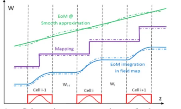
As schematically illustrated by Fig. 1, there are three different methods traditionally used to compute the longitudinal beam dynamics in linacs.

Figure 1 : Schematic representation of the energy evolution with the 3 methods used to compute the longitudinal dynamics : integration of the EoM in field maps (blue), mapping from cavity to cavity (violet), from the EoM obtained in smooth approximation (green).

The first method, by far the most accurate but computer-time consuming, consists in integrating the equation of motion (EoM) (1) using field maps giving the

amplitude of the rf accelerating field .

(1)

The second method consists in computing the evolution of the particle energies using the so-called Panofsky equation (2) [1] which gives the total energy gain produced by an accelerating gap or a cavity.

(2)

In (2), is the particle charge, the accelerating field

mean value, the gap or cavity length, the Transit

Time Factor (TTF) and the rf phase when the particle

crosses the gap or cavity center. The exact value of the TTF is given by (3) which shows that all the information concerning the field value along the particle trajectory

and the evolution of the particle “velocity” have

been transferred into the TTF.

(3)

Using (3) the computation of the particle energy evolution is even more complicated than using (1); the practical use of the Panofsky equation often used for linac designs requires therefore several approximations.

The first approximations consist in assuming that the

accelerating field seen by the particle is an

odd function of z and that the evolution of the particle radial position and velocity can be neglected. In this case the second integral of (3) vanishes and the TTF can be

expressed as a function of the particle radial position ( )

and “velocity” ( ) at the entrance of the gap or cavity (4).

(4) Under the form (4), the use of an analytical expression

of the accelerating field distribution allows a fast

computation of the TTF, then a fast computation of the particle energy evolutions using (2).

Eq. (4) has nevertheless the redhibitory drawback to produce non symplectic transformations inducing large spurious emittance growths [2]. The only way to build a simple symplectic mapping (5) is to use the synchronous

particle TTF ( ) for any particle, then to neglect

the effect of the particle velocity spread on the TTF. The error introduced by all these approximations can be very significant in the case of superconducting linacs with large energy gains per cavity and large energy spreads.

(5-1)

(5-2) The third method used to compute and understand the longitudinal dynamics consists in considering a

continuous longitudinal focalization (smooth

approximation). In this case the mixing of (5-1) and (5-2) leads to the second order differential equation (6) which describes the particle phase oscillations around the

synchronous particle. In (6) is the zero-current

longitudinal phase advance per unit of length and is

the damping coefficient which will be discussed later on.

(6)

TUPP064 Proceedings of LINAC2014, Geneva, Switzerland

04 Beam Dynamics, Extreme Beams, Sources and Beam Related Technologies 4A Beam Dynamics, Beam Simulations, Beam Transport

(3)

LONGITUDINAL BEAM DYNAMICS

WITHOUT DAMPING

The use of (6) with = 0 allows to study the main

properties of the longitudinal beam dynamics without damping (see [3] eg.). Fig. 2 gives an example showing the evolution of the separatrix shapes as a function of the synchronous phase and the evolution of the particle relative phase advances as a function of the phase oscillation amplitudes. The strongly nonlinear character of the longitudinal motion is well shown by these figures.

Figure 2 : From Eq. (6), separatrix shapes (left) and evolution of the particle relative phase advance as a function of their amplitude (right) for different synchronous phases from -15° (red) to -90° (brown).

The comparison between the dynamics obtained in the framework of the smooth approximation (6) with the one given by the mapping (5-1) and (5-2) must be done at a -90° synchronous phase to be in the undamped regime. This comparison does not show significant differences between both methods up to zero-current longitudinal

phase advances per focusing period of the order of =

50°. As shown in Fig. 3, a thin chaotic layer appears around the separatrix in the phase-space portrait obtained using the mapping at this value.

Figure 3 : = 50°/lattice phase-space portraits

Left : smooth approximation Eq. (6) Right : mapping Eq. (5-1) and (5-2)

The difference is more and more important when

increases as shown by the Fig. 4 phase-space portraits plotted using the mapping superimposed on the red separatrix calculated from the smooth approximation.

The study of the longitudinal beam dynamics using the mapping shows that the parametric resonances present in the stable region are always excited (Fig. 2 right hand side allows to estimate their positions). One can notice that the

1/4 resonance start to be excited at = 82° because at

this value calculated using the smooth approximation the real value of the phase advance per period is ~ 92°.

In addition, the lowest order resonances which are more

and more numerous in the separatrix area as

increases form a broader and broader chaotic sea leading to a higher and higher reduction of the longitudinal acceptance (a phenomenon described in [4] and [5]).

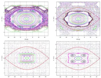
Figure 4 : Phase-space portraits from the mapping. From top left to bottom right :

= 60°/lattice (1/8 res.) = 70°/lattice (1/6 res.)

= 82°/lattice (1/4 res.) = 86°/lattice (1/4 res.)

The legitimate question arising looking to these results is “is this behaviour real or induced by the repetitive errors (which can be seen as a periodic excitation) done using the mapping?” or, in other terms, “is it a spurious

effect of the mapping?”

The answer is given by Fig. 5 which shows the phase-space portraits obtained making the integration of the EoM with the cavity “field map” given by Eq. (7).

(7)

Fig. 5 left which is the result of a calculation done without drift space between the cavities (lattice length = ), then with a purely sinusoidal field map, shows that such an accelerating field do not excite the resonances,

even at = 80°/lattice. At the opposite, Fig. 5 right

plotted with a lattice length = , then with a field map

with harmonics, shows that the resonances are excited by these harmonics which are always present in the mapping. One can notice the great similarities between the Fig. 4 (mapping) and Fig. 5 (EoM integration) phase-space

portraits at = 70°/lattice with the 1/6 resonance.

Figure 5 : Phase-space portraits from integration of the EoM in the “field map” (7)

Left : = 80°/lattice, purely sinusoidal field map

Right : = 70°/lattice, field map with harmonics

Proceedings of LINAC2014, Geneva, Switzerland TUPP064

(4)

LONGITUDINAL BEAM DYNAMICS

WITH DAMPING

The coefficient in (6) is given by (8), it is positive

when the beam is accelerated. In this case the particle phase oscillations are then damped and the attractor of the

stable trajectories in the (d , d ’) trace-space is the

central point (0, 0).

Fig. 6 gives two examples of such trajectories for a synchronous phase. Superimposed to the undamped separatrix in blue, the extreme stable trajectories in red and green define the basin of attraction (longitudinal acceptance with the classical golf-club shape). The size of this basin and the damping speed of

the trajectories increase rapidly as increases.

(8)

Figure 6 : (d , d ’) basin of attraction (smooth approx.)

, = 0.10 left and 0.50 right

When the (d , d ’) “trajectories” are plotted using the

mapping, Fig. 7 shows that, depending on their initial conditions, the particles are attracted either by the central point (0, 0) or by the resonance-island central points.

Figure 7 : (d , d ’) trajectories (mapping)

= 82°/lattice, = 0.02

This behaviour is well confirmed plotting the basin of

attractions for = 70° and 82°/lattice (Fig. 8 and 9

respectively). To plot these figures, at initial conditions

covering the whole (d , d ’) space, a red dot is plotted

when the motion is attracted by the central point and a green dot is plotted when the attractor is in the resonance islands.

To summarize we can say that the stable fix points of the resonance islands can act as main attractors at low damping rates but that the damping can annihilate the effect of the resonances. Anyway, the perturbation of the damping towards the central point (0, 0) leads to normalized emittance increase.

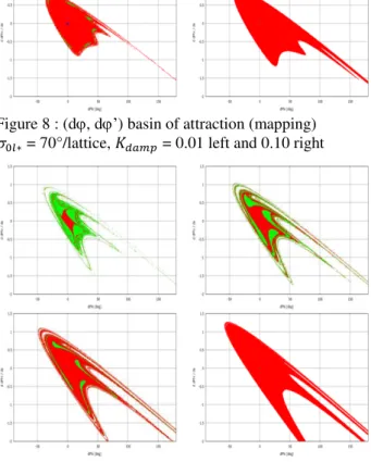
Figure 8 : (d , d ’) basin of attraction (mapping)

= 70°/lattice, = 0.01 left and 0.10 right

Figure 9 : (d , d ’) basin of attraction (mapping)

= 82°/lattice, from top left to bottom right :

= 0.01, 0.05, 0.10 and 0.20

SUMMARY

The zero-current longitudinal beam dynamics is complex; at least more complex than what is taught in classical accelerator books and accelerator schools!

The nonlinear character of the zero-current longitudinal dynamics is such that the parametric resonances affect the beam core and that there is strong longitudinal acceptance reductions as soon as the zero-current longitudinal phase advance is higher than 60°/lattice.

To understand the longitudinal beam dynamics in linacs it is essential to take into account the damping induced by the acceleration; the damping coefficient should be considered as an important parameter to analyze a linac design and understand its longitudinal beam dynamics.

REFERENCES

[1] W. Panofsky, “Linear accelerator beam dynamics”,

Lawrence Rad. Lab. Rep., UCRL report 1216, 1951.

[2] M. Promé, “Détermination de l’accélérateur linéaire

de 20 MeV, nouvel injecteur du synchrotron Saturne”, Rapport CEA-R-3261, Décembre 1968. [3] H. Bruck, “Accélérateurs circulaires de particules”,

INSTN, Presses Universitaires de France, 1966. [4] A. Fateev and P. Ostroumov, “The effect of drift

spaces on the longitudinal motion in an ion linac”, NIM Vol. 222 - Issue 3 - 1984.

[5] P. Bertrand, “Longitudinal resonances and emittance growth using QWR/HWR in a linac”, EPAC2004. -1.5 -1 -0.5 0 0.5 1 -50 0 50 100 150 dPhi (deg)

Damp_smooth_accept Longitudinal acceptance Phis = -30 deg K = 0.1 s max = 250

-1.5 -1 -0.5 0 0.5 1 -50 0 50 100 150 dPhi (deg)

Damp_smooth_accept Longitudinal acceptance Phis = -30 deg K = 0.5 s max = 250

TUPP064 Proceedings of LINAC2014, Geneva, Switzerland