Coding approaches for maintaining data in unreliable network systems

(1)

Coding Approaches for Maintaining Data in Unreliable

Network Systems

by

Vitaly Abdrashitov

B.S., Moscow Institute of Physics and Technology (2009) M.S., Moscow Institute of Physics and Technology (2011)

Submitted to the Department of Electrical Engineering and Computer Science in partial fulfillment of the requirements for the degree of

Doctor of Philosophy in Electrical Engineering and Computer Science at the

MASSACHUSETTS INSTITUTE OF TECHNOLOGY June 2018

c

Author . . . . Department of Electrical Engineering and Computer Science March 26, 2018

Certified by . . . . Muriel M´edard Cecil H. Green Professor in Electrical Engineering and Computer Science Thesis Supervisor

Accepted by. . . . Leslie A. Kolodziejski Professor of Electrical Engineering and Computer Science Chair, Department Committee on Graduate Students

(2)

(3)

Coding Approaches for Maintaining Data in Unreliable Network Systems by

Vitaly Abdrashitov

Submitted to the Department of Electrical Engineering and Computer Science on March 26, 2018, in partial fulfillment of the

requirements for the degree of

Doctor of Philosophy in Electrical Engineering and Computer Science

Abstract

In the recent years, the explosive growth of the data storage demand has made the storage cost a critically important factor in the design of distributed storage systems (DSS). At the same time, optimizing the storage cost is constrained by the reliability requirements. The goal of the thesis is to further study the fundamental limits of maintaining data fault tolerance in a DSS spread across a communication network. Particularly, we focus our attention on performing efficient storage node repair in a redundant erasure-coded storage with a low storage overhead. We consider two operating scenarios of the DSS.

First, we consider a clustered scenario, where individual nodes are grouped into clusters representing data centers, storage clouds of different service providers, racks, etc. The network bandwidth within a cluster is assumed to be cheap with respect to the bandwidth between nodes in different clusters. We extend the regenerating codes framework by Dimakis et al. [1] to the clustered topologies, and introduce generalized regenerating codes (GRC), which perform node repair using the helper data both from the local cluster and from other clusters. We show the optimal trade-off between the storage overhead and the inter-cluster repair bandwidth, along with optimal code constructions. In addition, we find the minimal amount of the intra-cluster repair bandwidth required for achieving a given point on the trade-off.

Second, we consider a scenario, where the underlying network features a highly varying topology. Such behavior is characteristic for peer-to-peer, content delivery, or ad-hoc mobile networks. Because of the limited and time-varying connectivity, the sources for node repair are scarce. We consider a stochastic model of failures in the storage, which also describes the random and opportunistic nature of selecting the sources for node repair. We show that, even though the repair opportunities are scarce, with a practically high probability, the data can be maintained for a large number of failures and repairs and for the time periods far exceeding a typical lifespan of the data. The thesis also analyzes a random linear network coded (RLNC) approach to operating in such variable networks and demonstrates its high achievable rates, outperforming that of regenerating codes, and robustness in a wide range of model and implementation assumptions and parameters such as code rate, field size, repair bandwidth, node distributions, etc.

Thesis Supervisor: Muriel M´edard

(4)

(5)

Acknowledgments

Pursuing my Ph.D. degree at MIT has been a long and challenging journey. At the same time, it has allowed me to meet many amazing and extraordinary people, students and faculty, inspiring researchers, innovative thinkers, dedicated teachers. I am deeply thankful to them for their support and sharing of the expertise.

First and foremost, I would like to thank Muriel M´edard, who has been to me not only an extremely knowledgeable and insightful research supervisor, but also a patient mentor, a very supportive adviser in career and life, and a wonderful person. Without her, I definitely would not have become what I am today.

Beside Muriel, I would like to thank Prakash Narayana Moorthy, with whom I enjoyed to be in a close collaboration, and who is a passionate researcher and a great friend. The thesis would not be possible without his extensive expertise. I am also honored to have David Karger and Viveck Cadambe as my committee members. I am really thankful for their time and commitment, and for the valuable guidance and advice.

I am extremely lucky to be a member of my research group of Network Coding and Reliable Communications. I would like to thank the people I met in the group for infinite opportunities to learn and share ideas. In particular, I would like to thank Ali Makhdoumi, Salman Salamatian, Weifei Zeng, Flavio du Pin Calmon, Ahmad Beirami, and Arman Rezaee for being supportive and true friends. I would also like to thank Surat Teerapittayanon, Georgios Angelopoulos, Kerim Fouli, Soheil Feizi, Jason Cloud, and many other members of the group, with whom I have had the pleasure to work and learn together. Very special thanks go to Molly Kruko, who makes sure that the group activities always run smoothly. I also wish to thank a lot of other great people who I met at MIT, and many of whom became my dearest friends.

Finally, and most importantly, I thank my parents and my family, for their unconditional love, support, and encouragement during all these years in the graduate school and in the U.S., and for being my backbone and foundation.

The work in this thesis was in part supported by the Air Force Office of Scientific Research (AFOSR) under award No FA9550-14-1-043 and FA9550-13-1-0023, in part supported by the National Science Foundation (NSF) under Grant No CCF-1527270 and CCF-1409228, and in part supported by the Defense Advanced Research Projects Agency (DARPA) award No HR0011-17-C-0050.

(6)

(7)

List of Figures

1-1 A system with n = 4 storage nodes with 2 packets per node, and a regenerating code, which can repair the exact content of any node by downloading 1 packet from each of 3 other nodes. The plus sign denotes bit xor operation. . . 17 1-2 Comparing the storage overhead and the expensive inter-cluster repair bandwidth

of three coding options for a clustered DSS. The three options are (i) extra parity check nodes in each cluster, (ii) classical regenerating codes, and (iii) generalized regenerating code. . . 20 1-3 An example of LRC with 6 information nodes and 4 parity nodes, 2 of which are

local parities. Every information node (e.g. c1) can be recovered by downloading

data from a specific set of d = 3 other nodes in the same local group. The global parities p1, p2are linear combinations of all 6 information symbols and allow data

regeneration when more than 1 node in each local group is lost. . . 21 1-4 The helper selection vs rate trade-off (higher the better). . . 22 1-5 Berlekamp’s bat phenomenon. . . 23 2-1 Storage-bandwidth trade-off for RCs with (n = 7, k = 5, d = 6, B = 10). The

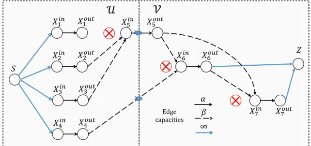
precise trade-off for exact repair remains unknown. . . 30 2-2 An example of information-flow graph for n = 4, k = 2, d = 2 and 3 node

failures/repairs. Also shown is a sample cut (U, V) between S and Z of capacity α + β. . . 31 3-1 An example of the IFG model representing the notion of generalized regenerating

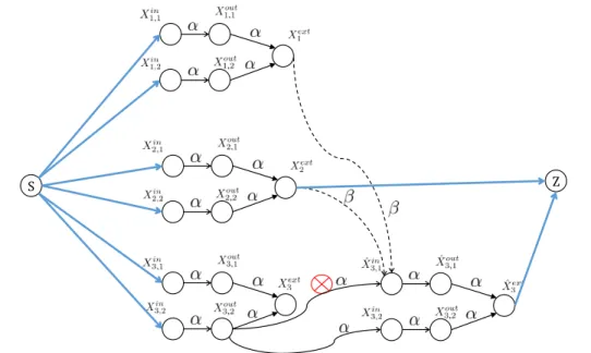
codes, when intra-cluster bandwidth is ignored. In this figure, we assume (n = 3, k = 2, d = 2)(m = 2, ℓ = 1). . . 38 3-2 An example of the information flow graph used in cut-set based upper bound for

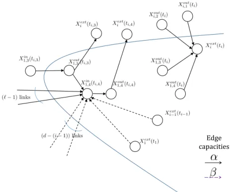
the file size. In this figure, we assume (n = 3, k = 2, d = 2)(m = 2, ℓ = 1). We also indicate a possible choice of S − Z cut that results in the desired upper bound. 42 3-3 An example of how any S −Z cut in the IFG affects nodes in Fi. In the example,

we assume m = 4. With respect to the description in the text, ai = 2. Further,

the node Xi,4(ti,4) is a replacement node in the IFG. . . 43

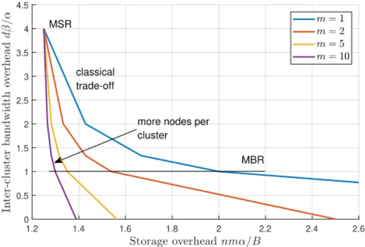
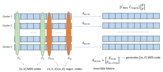
3-4 Trade-off between storage overhead nmα/B and inter-cluster repair bandwidth overhead dβ/α, for an (n = 5, k = 4, d = 4) clustered storage system, with ℓ = m − 1. . . 45 3-5 Illustration of the exact repair code construction. We first stack ℓ MDS codes

and (m − ℓ) classical regenerating codes, and then transform each row via the invertible matrix A. The first ℓ rows of the matrix A generates an (m, ℓ) MDS code. . . 48

(10)

3-6 An illustration of the node repair process for exact repair generalized regenerating code obtained in Construction 3.4.1. . . 50 4-1 An illustration of the information flow graph used in cut-set based upper bound

for the file-size under functional repair. We assume (n = 3, k = 2, d = 2)(m = 3, ℓ = 0, t = 2). Only a subset of nodes is named to avoid clutter. Two batches, each of t = 2 nodes, fail and get repaired first in cluster 1 and then in cluster 3. We also indicate a possible choice of the S − Z cut that results in the desired upper bound. We fail nodes in cluster 3 instead of cluster 2 only to make the figure compact. . . 59 4-2 Trade-offs for an (n = 5, k = 4, d = 4)(m = 3, ℓ = 0, t = 2) system, plotted

between the MSR and the MBR points. . . 63 4-3 Impact of number of local helper nodes, ℓ, on file-size for an (n = 7, k = 4, d = 5,

m = 17, t = 5) clustered storage system at MBR point (α = 1, β = 1). Local help does not provide any advantage unless ℓ > 2. . . 63 5-1 An illustration of the evolution of the k-th cluster of the information flow graph

used in cut-set based lower bound for γ in Theorem 5.1.1. In this figure, we assume that m = 4, ℓ = 2. Nodes 3, 4, 1 fail in this respective order. For the repair of node 3, nodes 1 and 2 act as the local helper nodes. For the repair of the remaining two nodes, nodes 2 and 3 act as the local helper nodes. Also indicated is our choice of the S-Z cut used in the bound derivation. . . 67 5-2 An illustration of the IFG used in cut-set based lower bound for γ′ _{in Theorem}

5.2.1. In this example, we assume (n = 3, k = 2, d = 2)(m = 2, ℓ = 1)(ℓ′ = 2, γ = α). The second node fails in clusters 1 and 2 in the respective order. Also indicated is our choice of the S-Z cut used in the bound derivation. . . 71 5-3 An illustration of the IFG used in cut-set based lower bound for ℓ′ in Theorem

5.2.3. In this example, we assume (n = 3, k = 2, d = 2)(m = 2, ℓ = 0)(ℓ′ _{= 1,}

γ = γ′ = α). The second node fails in clusters 1 and 2 in the respective order. Also indicated is our choice of the S-Z cut used in the bound derivation. . . 74 5-4 Simulation results for a system with parameters (n = 4, k = 3, d = 3), (ℓ = 1,

m = 2), (α, β = 4), showing probability of successful data collection against number of node repairs performed, for an RLNC-based GRC. The legends indi-cate parameters (γ, γ′, ℓ′) for each test. For all operating points ℓ∗= m = 2. . . 76 5-5 Illustrating the impact of ℓ on the various performance metrics. We operate at

the MBR point with parameters {(n = 12, k = 8, d = n−1)(α = dβ, β = 2)}. We see that while ℓ = m − 1 is ideal in terms of optimizing storage and inter-cluster BW, it imposes the maximum burden on intra-cluster BW. . . 77 6-1 An example of a system evolution for 3 iterations of failure and repair, n = 6,

d = 2, a = b = 1. At t = 0 node i contains packet si. For the 4 considered system

states the evolution matrix Wt _{and its matroid representation M(W}t_{) are also}

shown. The most recently changed column of Wtis bold-faced. . . 81 6-2 An example of information-flow graph for n = 4, d = 2 and t = 4 node

fail-ures/repairs. Also shown is a sample cut (U, V) of capacity a + 2b ≥ min{a, 2b} + min{a, b} + b. . . 93 6-3 Simulated expected lifetime for n = 20, a = b = 1. . . 96

(11)

6-4 Probability of decoding error pe against the coding rate for fixed n = 20, d = 4,

a = b = 1. The dots indicateE[rank Wt_{]/n. . . 96}

6-5 Expected rank of the evolution matrix rt=E[rank Wt], with the upper and lower

bounds for n = 40, d = 4. . . 97 6-6 Expected rank rt=E[rank Wt] for n = 40 and various values of d. . . 97

7-1 Performance of various recoding regimes: No recoding (N), Sparse recoding (S), and Full recoding (FR) for a system with parameters n = 20, t = 2000, d = 4, a = 3, b = 2. The legend indicates the recoding regimes (helper, replacement nodes). . . 100 7-2 Impact of the effective field size qa on the average rank of Wt for a system with

parameters n = 20, d = 4, a = b, t = 1000. The actual field size used is q. . . 100 7-3 Probability mass functions of the test node distributions for a storage with n = 20

nodes. Given a fixed parameter x, the probability of i-th atom is p(i) ∝ ix. Larger values of x lead to stronger concentration of probability at the nodes with high indices. . . 102 7-4 Impact of the failed and helper node distribution PF, PH on the average rank

for n = 20, t = 1000, d = 4. The distributions have p(i) ∝ ix _{for x ∈ {x}

F, xH}.

xF < 0 corresponds to p(i) ∝ (n + 1 − i)|xF|. . . 102

7-5 Impact of standard deviation of the number of helper nodes d on the average rank for n = 20, a = b = 1, t = 1000. Beta-binomial distributions with different supports are used. . . 103 7-6 Decoding error probability pdc_e = Pr[rank Mt|S < k| rank Mt = k] for randomly

chosen column set S ⊂ [n], |S| = ndc. n = 20, d = 4, a = b = 1, k = nR. . . 103

7-7 The maximal rate Rε for error probability under ε = 5 ∗ 10−4, t = 2000, and

n = 20. First, tests are performed for the base case a = b = 1, q = 65536, then, various adverse parameter changes are introduced incrementally. The maximal theoretical RC code rate for n = 20, a = 6, b = 4 is provided for comparison. . . . 105 8-1 Mean rank per node for t scaled proportionally to n with d = 4, a = b = 1. . . 110

(12)

(13)

List of Tables

3.1 Notation for the clustered storage system model. . . 36 6.1 Notation for the time-varying network storage system model. . . 82

(14)

(15)

Chapter 1

Introduction

1.1 Distributed Storage Systems

In the recent years, the demand for cheap and reliable data storage has been driven high by nu-merous entertainment, industrial, and scientific applications, which overall generate zettabytes (1 ZB ≈ 1012GB) of data yearly. In 2018 the size of the global data sphere is measured by tens of zettabytes, and this number doubles every 3 years [2]. The demand for the storage capacity grows faster than the storage media production and is expected to outstrip the production by 6 ZB in 2020 [3]. As a result of these trends, the storage cost becomes an increasingly important factor in the large storage systems design.

Large-scale storage systems follow a distributed approach: the data is spread across several storage nodes, possibly in different locations. Using multiple less capable and cheaper nodes instead of a single powerful node allows cost-efficient scalability. Thus, modern distributed storage systems (DSS) are composed of a large number of individually unreliable nodes. Data loss is unacceptable, and DSS must deal with failures in the system, i.e. have a sufficient fault tolerance.

Since fault tolerance is achieved through a redundancy in storage, and the redundancy inevitably increases the storage size per byte of user data, i.e. the storage overhead , it is critically important to find the optimal balance between the required fault tolerance and the storage cost. A simple way to introduce the redundancy is replication, in which multiple copies of the same data segments are stored on different physical nodes. Simple to set up and manage,

(16)

3-way replication (keeping 3 copies of data) has been a widely adopted approach. However, its storage overhead, is too high (3), and makes it prohibitively expensive for large amounts of data. An alternative approach to introduce redundancy is to encode the data using erasure codes. Storage node failures can be treated as erasures, and the source data can be decoded from an incomplete set of nodes. Many major cloud service providers like Amazon [4], Microsoft Azure [5] employ coding in their storage systems.

An important aspect in DSS is maintaining redundancy. Upon node failures, the data segments they store become unavailable, the overall redundancy and fault tolerance goes down. A new, replacement, nodes need to be introduced into the system to keep the failed portion of the data. This process is called node repair and involves downloading data (helper data) from a set of surviving nodes (helper nodes, or helpers) to generate the data to store on the new node. The efficiency of node repair is mainly associated with the following metrics:

1. repair bandwidth — the number of the symbols downloaded from the helper nodes to the replacement node [1];

2. repair locality — the number of the helper nodes contacted [6];

3. repair disk I/O — the number of stored symbols read by the helper nodes from their storage media to generate the helper data [7].

These metrics directly affect the repair latency, cost, and extra load on the helper nodes, and ideally, all the metrics should be small. However, the metrics can be simultaneously minimized only for a replication storage, but not for an erasure-coded DSS.

The thesis is focused on further studies of the fundamental limits of maintaining redundancy and node repair in DSS with a low storage overhead. We consider two operating scenarios of the DSS. The first one mainly considers DSS with a low repair bandwidth and disk I/O, while the second one studies a DSS with a low repair locality.

1.2 Small Repair Bandwidth

Repair bandwidth minimization has been largely studied in the context of regenerating codes (RCs). First introduced by Dimakis et al. [1], RCs require that repair of any node can be

(17)

a 1 a2 b1 b2 a₁ a₂ b1 b2 a₁+b1 a2+b2 a₁+b2 a2+b1 a1 b2 a₁+b1+a2+b2

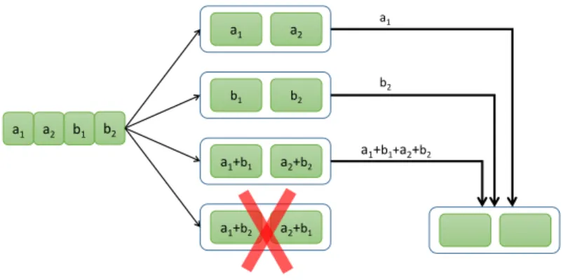
Figure 1-1: A system with n = 4 storage nodes with 2 packets per node, and a regenerating code, which can repair the exact content of any node by downloading 1 packet from each of 3 other nodes. The plus sign denotes bit xor operation.

performed with an arbitrary set of d helper nodes among the surviving nodes. For a fixed repair locality d, RCs minimize the repair bandwidth and achieve the optimal trade-off between the bandwidth and the storage overhead. Generally, to achieve the minimal repair bandwidth, a helper node needs to send a function of its stored data, rather than a part of it. Consider an example of a DSS with n = 4 storage nodes shown in Figure 1-1. The source file is split into 4 packets, represented by vectors of bits of a fixed dimension. They are encoded into 8 coded packets and stored on 4 nodes, 2 packets per node, so that the source file can be decoded from the content of any 2 nodes. To repair a failed node, e.g. node 4, the replacement node needs to download at least 3 helper packets from the other 3 nodes. It is not sufficient, however, for the helpers to directly send out the packets they store; instead helper node 3 sends out a linear combination a1+ b1+ a2+ b2 of packets a1+ b1, a2+ b2 it holds. The addition is performed

element-wise in the binary field GF (2). This demonstrates that network coding is necessary to achieve the minimal repair bandwidth.

Network coding refers to the operation of coding at a network node over its inputs to pro-duce its outputs. Whereas in the traditional paradigm of network routing, a node only stores the incoming packets to forward them to the next nodes without changing (possibly changing packets metadata), with network coding the node can emit packets which are functions, ”mix-tures” of the incoming packets. In the context of DSS, the incoming packets correspond to those a node stores, and the outgoing packets to those it sends out when it serves as a helper node.

(18)

The seminal work by Ahlswede et al. [8] shows that, unlike routing, network coding achieves the capacity of multicast wireline networks, where a data stream needs to be delivered to multiple destinations. The capacity is equal to the minimal value of a cut between the source node and a destination (a sink node). References [9, 10] showed that for achieving the multicast capacity it is sufficient to use linear network coding, where the outgoing packets are linear combinations of the incoming packets. Works of Ho et al. [11], Sanders et al. [12] showed that the linear coding coefficients at each node can be picked uniformly at random, and such random linear network codes (RLNC) in a large finite field asymptotically achieve the multicast capacity. Lin-ear network codes can also be constructed deterministically with a polynomial-time algorithm [13].

Dimakis et al. [1] considered two alternative repair regimes of RCs: exact (ER) and func-tional repair (FR). In ER regime after each node repair, the replacement node content should be exactly the same as the content of the failed node. With FR this does not need to hold, as long as the source file can be decoded. The advantage of the ER codes is that they can have a systematic form with certain nodes holding the uncoded source packets (the first two nodes in Figure 1-1), which allows very fast data reads. The FR codes generally achieve strictly better bandwidth-storage trade-off and allow simpler and more efficient code constructions. A detailed description of RCs and network coding is presented in Chapter 2.

Subsequent works on regenerating codes studied code constructions in specific capacity-achieving scenarios [14, 15], repairing multiple node failures [16–19], security aspects [20, 21]. These works consider the flat network topology, where each node has a direct logical connection to every other node, and all logical links incur the same bandwidth cost for communication per bit.

However, the practical large-scale DSSs feature hierarchical structure; for instance, individ-ual nodes can be grouped into a server rack and connected to the same network switch, while a rack is a part of an aisle, and the latter is a composition unit of a data center. Finally, data centers can be grouped into a geographically distributed storage system, employing erasure coding across data centers [22], or into a user-defined cloud-of-clouds along with other storage service providers [23–25]. In a large DSS, the data is protected against failure or unavailability of individual system parts, and repairing a node can require a repair traffic across different levels

(19)

of the system hierarchy. While the communication between the nodes in the same rack is low-delay and a spare bandwidth is usually available, the inter-rack bandwidth is shared by many nodes and applications and is a more limited resource, and the inter-data-center bandwidth is even more scarce and expensive. For instance, around 180TB of inter-rack repair bandwidth is used daily in the Facebook warehouse, which limits resources for other applications [26].

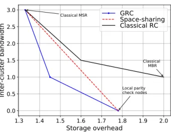
Although possible, complete elimination of the expensive, inter-cluster , as we shall call them, repair bandwidth components, e.g. by using extra parity check nodes in each rack, results in an excessively large storage overhead. A better approach is needed to characterize the optimal system performance in terms of the storage overhead vs repair bandwidth trade-off. The extra parity check solution is shown by the corresponding point on the trade-off in Figure 1-2. It is also possible to reduce the expensive bandwidth by employing several RCs for flat topologies (classical RCs), so that each RC spans across one node in each rack. Any point on the straight line between the two solutions can be achieved by space-sharing, i.e. applying each of the two codes only for a fraction of the total stored data.

We introduce Generalized Regenerating codes (GRCs) for clustered topologies, which care-fully combine repair bandwidth from different hierarchy levels (cheap intra-cluster and expen-sive inter-cluster bandwidths) to achieve the optimal trade-off. The trade-off is strictly better than what is achieved with space-sharing between the existing coding schemes, as shown in Figure 1-2. The analysis of GRCs is presented in Chapter 3. Besides the characterization of the optimal trade-off, we also provide explicit code constructions for the ER and the FR regime. The FR construction is optimal in terms of the trade-off, while the ER construction achieves the most important operating points of the trade-off. In Chapter 4 we extend the results to the scenario with multiple node failures per cluster and their simultaneous repair.

In Chapter 5 we study the local properties of GRCs. While the goal of GRC is to optimize the main trade-off between the storage vs the expensive inter-cluster bandwidth, it is also desirable to minimize the cheap intra-cluster bandwidth to improve the latency the disk I/O, without affecting the trade-off. The repair process also gives rise to the intra-cluster bandwidth in the clusters providing the helper data (helper clusters). The chapter gives the answer to the following question: what is the minimal intra-cluster bandwidth, in the cluster with the failed node and in the helper clusters, required to operate on a specific point of the trade-off?

(20)

1.3 1.4 1.5 1.6 1.7 1.8 1.9 2.0 Storage overhead 0.0 0.5 1.0 1.5 2.0 2.5 3.0 Inter-cl uster bandwidth Local parity check nodes Classical MBR Classical MSR GRC Space-sharing Classical RC

Figure 1-2: Comparing the storage overhead and the expensive inter-cluster repair bandwidth of three coding options for a clustered DSS. The three options are (i) extra parity check nodes in each cluster, (ii) classical regenerating codes, and (iii) generalized regenerating code.

1.3 Small Repair Locality

Optimizing the repair locality is typically studied in the context of locally repairable codes (LRCs). LRC-based solutions have been used in very large systems, like the storage for Microsoft Azure [5]. References [6, 27] first introduced the notion of LRC and demonstrated the trade-off between the locality, the minimum code distance, and the code rate (the inverse of the storage overhead) for linear or non-linear codes. Figure 1-3 shows an example of an LRC code which stores a file of 6 packets on 10 nodes. The 6 source packets are placed in the uncoded form on 6 information nodes, which belong to 2 local groups. Each local group contains d + 1 nodes and includes a local parity node, which allows exact regeneration of any information node from d = 3 helper nodes. Unlike the setting of RC, LRCs are mainly studied in the exact repair regime with a predetermined and fixed set of helper nodes (repair set) for each potential node failure. More recent studies [28–30] also considered LRCs in the functional repair regime and allowed the replacement node to choose the best repair set. The coding rate achievable by LRCs, where each symbol can be recovered by downloading data from d helper nodes, is bounded by

RLRC ≤

d

d + 1. (1.1)

(21)

a₁ a₂ b₁ b₂ c₁ c₂ a2 b2 c2 d₂=a₂+b₂+c₂ p₂ p₁ a₁ b₁ c₁ d₁=a₁+b₁+c₁

local group 1 local group 2

Figure 1-3: An example of LRC with 6 information nodes and 4 parity nodes, 2 of which are local parities. Every information node (e.g. c1) can be recovered by downloading data from a

specific set of d = 3 other nodes in the same local group. The global parities p1, p2 are linear

combinations of all 6 information symbols and allow data regeneration when more than 1 node in each local group is lost.

access to the specific repair set from the replacement node cannot be guaranteed because of (temporarily) helper nodes unavailability, which may be caused by the node maintenance, unresponsiveness due to high load, bandwidth over-subscription, network congestion, etc. This issue is of a special importance in networks with highly unstable or time-varying topology, such as peer-to-peer (P2P) and peer-aided edge/fog caching networks, mobile ad hoc, and sensor networks. The problem does not arise for RCs and MDS codes, where an arbitrary set of d nodes can serve as helpers, but those codes have significantly lower coding rate RRC ≤ d/n, for a

storage with n nodes. Works [31, 32] and others considered LRCs with several alternative repair sets. Specifically, [31] considered local groups of d+δ −1 nodes, such that a node within a group can be recovered from any subset of d other nodes in a group. Each local group represents an MDS code with the minimum distance δ ≥ 2. Although this construction increases the maximal coding rate to _d+δ−1d , the repair is still bound to a local set of a relatively small number of nodes. A different model is considered by reference [32]: the nodes have multiple, τ ≥ 1, disjoint repair sets of size d, and the resulting coding rate is upper-bounded by Qτ_i=1(1 + 1/di)−1_{. While this}

gives a coding rate improvement as compared to RCs, τ cannot be large, and the repair set selection remains limited with many nodes excluded from the consideration to be helpers.

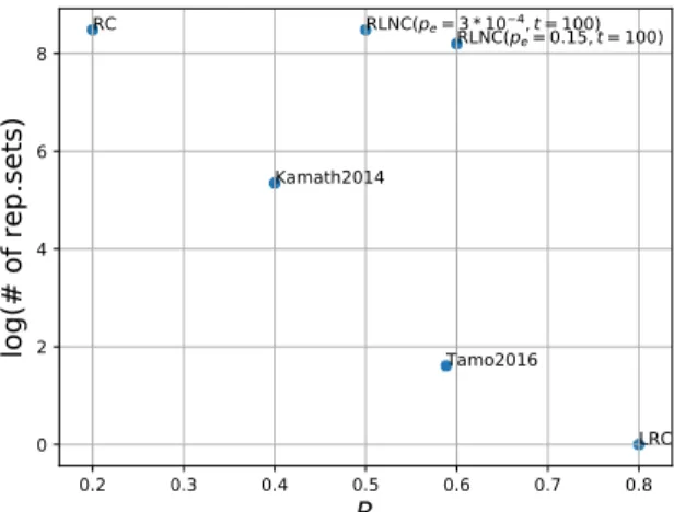
Fundamentally, LRCs can achieve a high rate at the price of a limited helper selection and a small minimum code distance, while the large minimum distance of RC and MDS codes allows an arbitrary choice of helpers at the price of a low rate (Figure 1-4). The minimum distance is often treated as the key code parameter controlling the fault tolerance of the DSS. However, it only measures the fault tolerance with respect to the worst-case erasure patterns, while these

(22)

0.2 0.3 0.4 0.5 0.6 0.7 0.8 R 0 2 4 6 8

log

(#

of

rep

.se

ts)

RC Kamath2014 Tamo2016 LRC RLNC(pe=3*10_RLNC(4,t=100) pe=0.15,t=100)

Figure 1-4: The helper selection vs rate trade-off (higher the better).

patterns constitute only a small fraction of the possible patterns. Since the DSS reliability is typically compared via expected value metrics (e.g. normalized magnitude of data loss — the expected number of lost bytes per terabyte in the first 5 years of deployment [33]), it is more natural to consider the expected impact of the potential failure and repair availability patterns on the storage. In channel coding, this phenomenon is illustrated with the Berlekamp’s bat [34, Chapter 13] (Figure 1-5. A bat flies around the center of a nearly-spherical cave, the center of which represents the original codeword surrounded by the neighboring codewords in a high-dimensional code space. The location of the bat represents the distorted codeword. The bat tries to avoid touching the pikes from the wall. Since neighboring codewords exactly at the minimum distance are scarce, the range at which she can fly in the perfect safety is far less than the actual range she can fly with a high probability of safety. While the early coding theory focused on codes with a large minimum distance which guarantee to correct a large number of erasures, the Shannon capacity can only be reached by the codes working far beyond the minimum distance of the code: the probability of hitting the vicinity of another codeword is low even when the number of erasures exceeds the minimum distance. Examples of such codes are Turbo codes, LDPC, and random linear codes.

To study the expected impact of failures and repairs, we need to introduce a probability measure on them, i.e. to consider a random selection of the failure and helper nodes. Since in channel coding random linear codes perform well in decoding beyond the minimum distance, for

(23)

Perfect safety range

Safety range with high probability

Figure 1-5: Berlekamp’s bat phenomenon.

a random selection DSS model it is most natural to repair a node by generating random linear combinations of the packets on the helper nodes, in other words, employing RLNC. In Chapter 6, we introduce a stochastic failure and repair DSS model, equipped with an RLNC code generation and repair, and study its rate-reliability trade-offs. Since the model is probabilistic, its performance is parametrized by time, which is measured as the number of the failure and repair iterations.

The time-dependent nature of the model has another interesting aspect. Most existing DSS codes, such as MDS, RCs, and LRCs, are designed under the assumption that the data needs to be stored forever. However, the data often has a limited lifespan, after which the data can be deleted or migrated to another (e.g. archival) storage. The lifespan can be really short: for instance, in edge caching, a certain content can be popular just for a month, and afterwards it does not need to be stored in caches any more. For such scenarios, it is reasonable to have a code which provides the guarantees of maintaining the data only for a limited number of node repairs. As a result of this relaxed requirements, we can expect an improved storage overhead and lower storage costs. The RLNC code considered in Chapter 6 with a gradual degradation over time under a random node selection model is well-suited for such limited lifetime applications. The code both realizes the rate gain over RCs and has practically the same helper selection freedom as RCs, far exceeding that of LRCs (Figure 1-4), which makes it a viable storage solution for the time-varying networks.

(24)

In Chapter 7, we numerically study the performance of RLNC under our model in a wide range of model and implementation assumptions and parameters. We show RLNC to perform stably well with the binary field, low repair bandwidth, non-uniform node distributions, variable number of helper nodes, and sparse RLNC recoding. Even in those adverse conditions, the achievable code rate is shown to be significantly higher than that of regenerating codes.

(25)

Chapter 2

Preliminaries

In this chapter, we provide the notations and tools used throughout the thesis. We give the basic definitions of the coding theory, network coding, and the matroid theory. In addition, we provide an overview of the framework and main results from the theory of RCs, and introduce information flow graphs (IFG) as an important tool for studying functional repair systems.

2.1 Notations

Unless indicated otherwise, we use capital letters to denote matrices, sets and graph node labels, bold small letters to denote row vectors, and regular font for scalar variables. We also use capital letters when we need to highlight the fact that a variable is a random variable. rowspan A and colspan A denote the linear subspaces spanned by rows and columns of matrix A, respectively. Indenotes the n × n identity matrix. AT denotes the transposition of a matrix

or a vector A. Unless specified otherwise, A|s_{, A|}S _{denote the submatrices of A consisting of}

row s, rows in set S, respectively. A|s, A|S denote the submatrices of A consisting of column s,

columns in set S, respectively.

|A| is the cardinality of set A. We use A ∪ B, A ∩ B, A − B to denote union, intersection, and set-theoretic difference of sets A, B, and also use A + b, A − b to denote A ∪ {b}, A − {b}. The set of integers between i, j inclusive is denoted [i, j] = {i, i+1, . . . , j −1, j], and [n] , [1, n]. Unless specified otherwise, all data/code symbols are considered elements of a finite field Fq. We useFq to denote any finite field with q non-zero elements. Whenever needed, a specific

(26)

field will be indicated, if multiple fields with the same q exist (for non-prime q). H(X) will denote the entropy of a discrete random variable or a set of random variables X, computed with respect to log q. H(X|Y ) denotes the conditional entropy. We shall also use the chain rule entropy expansion: H(X1, X2, . . . , Xn) = n X i=1 H(Xi|{Xj, j ∈ [i − 1]}). (2.1)

For a real number x, (x)+ _{is used as a shorthand notation for max{x, 0}. For integers a, b, if b} is a multiple of a, we shall write a|b, and a ∤ b otherwise. 1E is the indicator function, equal to

1 if E is true, and 0 otherwise.

For a system of equations or inequalities, notation     A B (2.2)

implies that at least one among A, B must hold true.

2.2 Linear Codes

A brief overview of the main notions in coding theory is given in this section. For a more detailed reference on the topic, we refer the readers to [35].

A (block) code C is a map from Fkq toFnq. In this thesis we only consider linear (n, k) codes,

for which the map is described by a linear transformation C : u → uG, where full-rank matrix G ∈ F Fqk×n is called generator matrix of the code. u is referred to as a vector of information

symbols or a message, uG is a codeword corresponding to the message. The set of all possible codewords forms the codebook, which with a slight abuse of notation will be also denoted by C = {uG}u_∈Fk

q. Note, that for any codewords c, c

′ _{∈ C and any a ∈ F}

q, ac and c + c′ also

belong to C, i.e. the code can also be characterized as a linear subspace of Fn

q with dimension

k. The codebook is not uniquely identified with the generator matrix, for any full-rank matrix A ∈ Fk×kq , a code with generator matrix AG corresponds to the same codebook.

(27)

codeword symbol. The code is called systematic if the generator matrix is of the form G = [IkP ]; in this case, the first k codeword symbols contain the original message symbols, and the

remaining n − k are parity check symbols.

The weight |x| of a codeword x is the number of non-zero symbols in it, and the (Hamming) distance |x − x′_{| between two codewords x, x}′_{, is the weight of their difference, i.e. the number}

of the coordinates where the two codewords differ. The minimum distance of code C is the shortest distance between two distinct codewords from C, or equivalently, the smallest weight of a non-zero codeword in C. The minimum distance D ≤ 1 of the code is related to the code capability to tolerate symbol erasures. If a codeword x = uG suffers erasures at m arbitrary positions, the observed codeword y has m coordinates unknown, but it can be corrected and uniquely mapped back to x and decoded to u as long no other codeword x′ _{can be transformed}

to y by m erasures. A code with minimum distance D can correct arbitrary D − 1 erasures in a codeword. Such code is called a (n, k, D) code.

Theorem 2.2.1 (Singleton Bound). The minimum distance of a (n, k) linear code is upper bounded by

D ≤ n − k + 1. (2.3)

A code that achieves the Singleton bound with D = n − k + 1 is called maximum distance separable (MDS). For an MDS code every subset of k columns of the generator matrix is linearly independent, and therefore any k symbols of a codeword x are sufficient to decode the message u.

Theorem 2.2.2 (MDS Code Generate Matrix). A code is MDS if and only if its codebook can be represented by a generator matrix in the systematic form G = [Ik P ], and every square

sub-matrix of P is invertible, where a sub-matrix is defined as an intersection of any i columns with any i rows, i ∈ [min{k, n − k}].

Examples of MDS codes are:

• n-Repetition code (n, 1, n);

(28)

• Reed-Solomon (RS) codes (n, k, n − k + 1).

While the first two codes can be constructed overF2, RS codes requireFq with q ≥ n.

For systematic codes C1(n1, k1), C2(n2, k2) with generator matrices, G1 = [Ik1 P1], G2 =

[Ik2 P2], the product code C(n2n1, k2k1) of C1, C2 maps a message U ∈ F

k2×k1 q to a codeword X ∈ Fn2×n1 q , where X is given by X =    U U P1 P₂TU P₂TU P1    =    U P₂TU    [Ik1 P1] =   Ik2 P₂T    [U UP1]. (2.4)

Every row of X is a codeword from C1, and every column is a codeword from C2.

For integer α ≥ 1, a linear (n, k) vector code C is a linear (n, k) code over symbol alphabet Fα

q, such that its codewords are Fq-linear, i.e. for any codewords c, c′ ∈ C and any a, a′ ∈ Fq,

ac + a′_c′ _{∈ C.}

2.3 Linear Network Coding

Network coding in packet networks assumes that intermediate nodes perform coding across the incoming packets to generate the outgoing packets. Specifically, in this thesis we assume that in a network with packets of length m′, a node x with k incoming and n outgoing links computes n outgoing packets as the columns of U Gx, where matrix U ∈ Fmq′×k contains the k incoming

packets as columns, and Gx ∈ Fk×nq is the generator matrix of a local linear code at node x;

note that n is determined by the network structure, and may be smaller than k. We will say that node x recodes the k incoming packets into n outgoing packets. In random linear network coding (RLNC) the elements of Gxare drawn at random fromFq, rather than deterministically

constructed based on the network topology.

To keep track of the transformations of the original source packets after several recoding operations, each coded packet has a header with the coordinates in the source packets basis. To be more precise, let s1, . . . , sr ∈ Fm_q be uncoded source packets to be transmitted over the

(29)

network, let matrix S , [s1T. . . srT] ∈ Fm×r_q , and let S′ =   Ir S    . (2.5)

The columns of S′ are injected into the network as packets of length m′ = r + m, with an r-symbol header. When these packets are recoded in the network, each generated coded packet is a linear combination of columns of S′, in which the first r symbols are the coordinates of the m-symbol payload part in the basis of the source packets s1, . . . , sr. The r-symbol header

is called (global) coding vector of the packet. Whenever a node receives r coded packets with linearly independent coding vectors, i.e. the matrix of the r coding vectors is full-rank, the node can decode the r source packets by applying the inverse linear transformation to the received packets.

2.4 Regenerating Codes

Next, we overview the model of RCs of [1]. A source file of size B symbols is encoded and stored in a DSS of n storage nodes. Each node stored α symbols, and the code rate is B/nα. Whenever a node failure happens, a new node replaces the failed one and downloads β symbols of helper data from each node from an arbitrary set of d ≥ k helper nodes to generate its content. Under exact repair (ER) the generated content should be the same as that on the failed node, under functional repair (FR) there is no such constraint. To retrieve the source file (perform data collection) one downloads the content of an arbitrary set of k nodes.

For the model outlined above with parameters (n, k, d, α, β) and FR, the source file of size B can be stored in the system if and only if

B ≤ BF R , k

X

i=1

min{α, (d − i + 1)β}. (2.6)

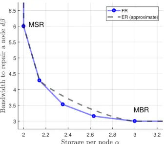
For a fixed file size B, there exists a trade-off between storage α per node and repair bandwidth dβ (Figure 2-1. Only the pairs of (α, dβ) on or above the trade-off curve are feasible.

(30)

2 2.2 2.4 2.6 2.8 3 3.2 3 3.5 4 4.5 5 5.5 6 6.5 FR ER (approximate) MBR MSR

Figure 2-1: Storage-bandwidth trade-off for RCs with (n = 7, k = 5, d = 6, B = 10). The precise trade-off for exact repair remains unknown.

Since α is proportional to the storage overhead nα/B, lower values of α lead to lower storage costs. The MSR (minimum storage regeneration) point on the trade-off corresponds to the smallest storage overhead, and is defined by α = B/k = (d − k + 1)β. The MBR (minimum bandwidth regeneration) point on the trade-off corresponds to the smallest repair bandwidth, which is defined by dβ = α, B =Pk_i=1_{(d − i + 1)β. For a bounded number of failures, all points} on the FR trade-off can be achieved by linear network coding over a large enough field, or in particular by RLNC, or space-sharing of two network coded solutions. Reference [36] presented randomized and deterministic FR code constructions for an unlimited number of failures. The general ER trade-off remains an open problem, although it is known that ER can always achieve the MSR and MBR points, and for most points between those two the ER trade-off is strictly worse than that of FR. Under ER, the MBR point can be achieved by a product-matrix code construction for all values of parameters (n, k, d) [14].

2.4.1 Information Flow Graph

Information flow graph (IFG) is a convenient tool for analysis of the maximal achievable file size of RC models in FR regime. The IFG is a directed acyclic graph with capacitated edges, which represents the data flows from the uncoded source file to the data collectors via an error-free network of the original and replacement storage nodes with limited memory. Each original or

(31)

𝑋𝑖 _𝑋 𝑋𝑖 _𝑋 𝑋𝑖 _𝑋 𝑋𝑖 𝑋 𝑋𝑖 _𝑋 𝑋𝑖 _𝑋 𝑋𝑖 _𝑋 Edge capacities ∞ 𝑍 𝑆

Figure 2-2: An example of information-flow graph for n = 4, k = 2, d = 2 and 3 node fail-ures/repairs. Also shown is a sample cut (U, V) between S and Z of capacity α + β.

replacement physical node Xi of size α is represented in the IFG by a new pair of in- and

out-graph nodes Xin i

α

→ Xout

i with an edge of capacity α between them. The in-node represents the

single point, where data enters to the node, possibly from several sources, e.g. helper nodes. The out-node connects to the other nodes or data collectors, where node Xi sends data. A

special IFG node S serves as the source of the source file of size B to be stored in the DSS. The IFG evolves with the DSS as node failures and repairs happen. Before any node failures, IFG contains n pairs of nodes X_iin, X_iout_{, i ∈ [n], and all n out-nodes are considered active. The} source node S connects to all the n in-nodes X_iin_{, i ∈ [n] via edges of infinite capacity. If node} Xi fails, its IFG out-node Xiout becomes inactive, a replacement physical node is introduced to

the system, and downloads helper data from some d surviving nodes. The new node has a new index, say Xn+1, and is represented by a new pair of the in- and the out-node in the IFG. The

in-node Xin

n+1 connects to the corresponding d active out-nodes via edges of capacity β. The

new out-node Xout

n+1 becomes active, so that at any moment there are n active out-nodes in the

graph. A data collector is represented by a node Z, which connects to the n active out-nodes X_jout at any specific moment via edges of infinite capacity. An example of IFG is shown in Figure 2-2.

(32)

corresponding to a cut (U, V) is the set of all edges which go from a node in U to a node in V. The capacity (or the value) of a cut or the corresponding cut-set is the sum of the capacities of the edges in the cut-set. A cut between nodes S and Z is any cut (U, V) with S ∈ U, Z ∈ V. If S is a proper cut-set between S, Z, then any directed path from S to Z has at least one edge in S. A cut between S, Z is called a minimal cut or min-cut, if its capacity is minimal among all cuts between S and Z.

Given parameters (n, k, d, α, β, B), the problem of code repair satisfying the RC model requirements can be cast as a problem of multicasting B symbols over all possible IFGs with parameters (n, d, α, β) to an arbitrary number of data collectors, connecting to any k active out-nodes. The latter problem is solvable if and only if B is no greater than the min-cut value between S and any data collector node Z for any possible IFG. Moreover, if the condition is satisfied, then there exists a linear network code solution over a sufficiently large field such that all data collectors can recover the B source symbols. RLNC also provides a solution with an arbitrarily large probability as the field size increases for a bounded number of failures/repairs.

2.5 Matroids

In this section, we give a brief overview of the matroid theory terminology and results used in the thesis. We refer the reader to reference [37] for more details.

A matroid M is a pair (E, I) consisting of a finite set E (the ground set), and a collection I of subsets of E. The elements of I are called independent sets. I should satisfy the following properties:

• I is non-empty.

• Every subset of an independent set is also independent.

• (Independence augmentation property) If sets I1 and I2 are independent (I1, I2 ∈ I), and

|I2| = |I1| + 1, then there is an element s ∈ I2− I1, such that I1∪ {s} is independent.

A set S ⊆ E which is not independent is called dependent. The maximal independent sets are called bases (I ∈ I, I + s /∈ I, ∀s /∈ I). Every basis has the same cardinality. The minimal dependent sets are called circuits (S /_{∈ I, S − s ∈ I, ∀s ∈ S). A matroid on n elements}

(33)

is uniquely characterized not only by the collection of its independent sets but also by the collection of its circuits. An element s ∈ E is a loop if it is not an element of any basis, or, equivalently, if {s} is a circuit. An element s ∈ E is a coloop if it is not an element of any circuit, or, equivalently, if s is an element of every basis. If for elements s1, s2 of matroid M,

{s1, s2} is a circuit, then s1 and s2 are said to be parallel in M, and the set of all elements

parallel to s1 or s2 is called a parallel class.

Given a matrix A ∈ Fn×m

q , the vector matroid M[A] is the matroid defined over the set of

columns of A, where a subset independence is defined as the linear independence of the columns in the subset.

If out of the three properties of I only the first two are satisfied, the resulting object (E, I) is called an independence system.

(34)

Part I

Regenerating Codes for Clustered

Storage Systems

(35)

Chapter 3

Generalized Regenerating Codes

(GRCs) and File Size Bounds

3.1 System Model

We propose a natural generalization of the setting of regenerating codes (RC) [1] for clustered storage networks. The network consists of n clusters, with m nodes in each cluster. The network is fully connected such that any two nodes within a cluster are connected via an intra-cluster link, and any two clusters are connected via an inter-cluster link. A node in one cluster that needs to communicate with another node in a second cluster does so via the corresponding inter-cluster link. A source file of size B symbols is encoded into nmα symbols and stored across the nm nodes such that each node stores α symbols. For data collection, we have an availability constraint such that the entire content of any k clusters should be sufficient to recover the original data file. Nodes represent points of failure. In this chapter, we restrict ourselves to the case of efficient recovery from single node failure. In Chapter 4, we generalize some of our results to the scenario of recovering from multiple node failures within a cluster.

Node repair is parametrized by three parameters d, β and ℓ. We assume that the replacement of a failed node is in the same cluster (host cluster ) as the failed node. The replacement node downloads β symbols each from any set of d other clusters, dubbed remote helper clusters. The β symbols from any of the remote helper clusters are a function of the mα symbols present

(36)

Table 3.1: Notation for the clustered storage system model. Symbol Definition

B source file size

n total number of clusters in the system m number of storage nodes in each cluster k number of clusters required for data collection

d number of remote helper clusters providing helper data during a node repair

d′ _{min{d, k}}

ℓ number of local helper nodes providing helper data during node repair q finite field size for data symbols

α number of symbols each storage node holds for one coded file

β size of helper data downloaded from each remote helper cluster during node repair, in symbols

in the cluster; we assume that a dedicated compute unit in the cluster takes responsibility for computing these β symbols before passing them outside the cluster. In addition, the replacement node can download (entire) content from any set of ℓ ∈ [m − 1] other nodes, dubbed local helper nodes, in the host cluster, during the repair process. The quantity dβ represents the inter-cluster repair-bandwidth. We shall also use notation d′ _{= min{d, k}. We refer to the overall}

code as the generalized regenerating code (GRC) Cm with parameters {(n, k, d)(α, β)(m, ℓ)}. A

summary of the various parameters used in the description of the system model appears in Table 3.1.

The model reduces to the setup of RCs in [1], when m = 1 (in which case, ℓ = 0 automat-ically). We shall refer to the setup in [1] as the classical setup or classical regenerating codes. Our generalization has two additional parameters ℓ and m when compared with the classical setup. As in the classical setup, we consider both FR and ER regimes. We further note that, unlike the classical setup, our generalized setup permits d < k.

We will say that a GRC code is locally non-redundant if the encoding function does not introduce any local dependence among the content of the various nodes of a cluster. For linear GRC, the coded content of cluster i can be written as uGi, where u is the message vector of

length B, and Gi is a B × mα matrix. In this case, locally non-redundant code means that

Gi has full column rank. Oppositely, a locally redundant code can have, for example, a local

parity node within a cluster, which would hold the component-wise sum in Fα

q of the data on

(37)

The model described above does not consider intra-cluster bandwidth incurred during repair. Intra-cluster bandwidth is needed, firstly, to compute the β symbols in any remote helper cluster, and, secondly, to download content from ℓ local helper nodes in the host cluster. The intra-cluster bandwidth of GRC is studied in detail in chapter 5.

Our goal is to obtain a trade-off between storage overhead nmα/B and inter-cluster repair-bandwidth dβ for an {(n, k, d)(α, β)(m, ℓ)} GRC.

3.1.1 IFG Model for GRC

In this section, we describe the IFG model of GRC used in this chapter to derive the main file size bound. Let Xi,j denote the physical node j ∈ [m] in cluster i ∈ [n]. In the IFG, Xi,j is

represented by a pair of nodes X_i,jin _{→ X}α _i,jout. With a slight abuse of notation, we will let Xi,j to

also denote the pair (X_i,jin, X_i,jout) of the graph nodes. Cluster i also has an additional external node, denoted as X_iext. Each out-node in the cluster X_i,jout_{, j ∈ [m] is connected to X}_iext via an edge of capacity α. The external node Xext

i is used to transfer data outside the cluster, and

thus serves two purposes: 1) it represents a single point of contact to the cluster, for a data collector which connects to this cluster, and 2) it represents the compute unit which generates the β symbols for repair of any node in a different cluster.

The source node S connects to the in-nodes of all physical storage nodes in their original state (S _{→ X}∞ _i,jin_{), ∀i ∈ [n], ∀j ∈ [m]. The sink node Z represents a data collector, it connects to} the external nodes of an arbitrary subset of k clusters (X_iext _{→ Z).}∞

Each cluster at any moment has m active nodes. When a physical node Xi,j fails, it

becomes inactive, and its replacement node, say bXi,j, becomes active instead (see Figure 3-1

for an illustration). The replacement node bXi,j is regenerated by downloading β symbols from

any d nodes in the set {Xext

i′ , i′ ∈ [n], i′ 6= i}. The replacement node also connects to any subset

of ℓ nodes in the set {Xout

i,j′, j′ ∈ [m], j′ 6= j} via links of capacity α.

Along with the replacement of Xi,j with bXi,j, we will also copy the remaining m − 1 nodes

in cluster i as they are, and represent them with new identical pairs of nodes (X_i,jin′

α

→ Xi,jout′),

j′_{∈ [m], j}′ _{6= j. We shall also a have a new external node for the cluster, which connects to the} new m out-nodes. Thus, in the IFG modeling, we say that the entire old cluster with the failed node becomes inactive, and gets replaced by a new active cluster. For either data collection

(38)

S Z

Figure 3-1: An example of the IFG model representing the notion of generalized regenerating codes, when intra-cluster bandwidth is ignored. In this figure, we assume (n = 3, k = 2, d = 2)(m = 2, ℓ = 1).

or repair, we connect to external nodes of the active clusters. Note that, at any point in time, a physical cluster contains only one active cluster in the IFG, and fi inactive clusters in the

IFG, where fi≥ 0 denotes the total number of failures and repairs experienced by the various

nodes in the cluster. We shall use the notation Xi(t), 0 ≤ t ≤ fi to denote the cluster that

appears in IFG after the tth _{repair associated with cluster i. The clusters X}i(0), . . . , Xi(fi− 1)

are inactive, while Xi(fi) is active, after fi repairs. The nodes of Xi(t) will be denoted by

X_i,jin(t), X_i,jout(t), X_iext_{(t), 1 ≤ j ≤ m. With a slight abuse of notation, we will let X}i(t) to also

denote the collection of all 2m + 1 nodes in this cluster. We write Xi,j(t) to denote the pair

(Xin

i,j(t), Xi,jout(t)); again, with a slight abuse of notation, we shall use Xi,j(t) to also denote the

node j in cluster i after the tth _{repair in cluster i. We further use notation F}

i to denote the

union (family) of all nodes in all inactive clusters, and the active cluster, corresponding to the physical cluster i after t repairs in cluster i, i.e., Fi = ∪ft=0i Xi(t). We have avoided indexing Fi

with the parameter t as well, to keep the notation simple. The value of t in our usage of the notation Fi will be clear from the context.

(39)

3.2 Previous Work

Regenerating code variations for the data-center-like topologies consisting of racks and nodes are considered in [38–42]. In [38], [39] and [40], the authors distinguish between inter-rack (inter-cluster) and intra-rack (intra-cluster) bandwidth costs. Further, the works [38] and [39] permit pooling of intra-rack helper data to decrease inter-rack bandwidth. Also, all three works allow taking help from host-rack nodes during repair. Unlike our model, for data collection, all three works simply require file decodability from any set of k nodes irrespective of the racks (clusters) to which they belong. In other words, the notion of clustering applies only to repair, and not data collection, and this is a major difference with respect to our model. Thus, while these variations are suitable for modeling the node-rack topologies present within a data center, they do not model the situation of erasure coding across data centers with the availability requirement as considered in this work. The work in [41] is a variation of that in [40] for a two-rack model, where the per-node storage capacity of the two racks differ. In [42], the authors consider a two-layer storage setting like ours, consisting of several blocks (analogous to clusters as considered in this work) of storage nodes. A different clustering approach is followed for both data collection and node repair. For data collection, one accesses kc nodes each from

any of bc blocks. Though [42] focuses on node repair, the model assumes possible unavailability

of the whole block where the failed node resides, and as such uses only nodes from other blocks for repair. Further, unlike our model in this work, the authors do not differentiate between inter-block and intra-block bandwidth costs. The framework of twin-codes introduced in [43] is also related to our model and implicitly contains the notion of clustering. In [43] nodes are divided into two sets. For data collection, one connects to any k nodes in the same set. Recovery of a failed node in one set is accomplished by connecting to d nodes in the other set. However, there is no distinction between intra-set and inter-set bandwidth costs, and this becomes the main difference with our model.

Several works [44–49] study variations of RCs in varied settings, with different combinations of node capacities, link costs, and amount of data-download-per-node. The main difference between our model and these works is that none of them explicitly considers clustering of nodes while performing data collection. In [44], the authors introduce flexible regenerating codes for

(40)

a flat topology of storage nodes, where uniformity of download is enforced neither during data collection nor during node repair. References [45], [46] consider systems where the storage and repair-download costs are non-uniform across the various nodes. The authors of [45], as in [44], allow a replacement node to download an arbitrary amount of data from each helper node. In [47], nodes are divided into two sets, based on the cost incurred while these nodes aid during repair. As noted in [41], the repair model of [47] is different from a clustered network, where the repair cost incurred by a specific helper node depends on which cluster the replacement node belongs to. The works of [48] and [49] focus on minimizing regeneration time rather regeneration bandwidth in systems with non-uniform point-to-point link capacities. Essentially, each helper node is expected to find the optimal path, perhaps via other intermediate nodes, to the replacement node such that the various link capacities are used in a way to transfer all the helper data needed for repair in the shortest possible time. It is interesting to note both of these works permit pooling of data at an intermediate node, which gathers and processes any relayed data with its own helper data. Recall that our model (and the one in [38]) also considers pooling of data within a remote helper cluster, before passing on to the target cluster.

3.3 File Size Bound

In this section, we derive a bound for file size B for an arbitrary set of code parameters. We further use this bound to characterize the storage overhead vs inter-cluster repair bandwidth overhead trade-off.

Theorem 3.3.1 (GRC Capacity). The file size B of GRC with parameters {(n, k, d) (α, β) (m, ℓ)} under FR regime is upper bounded by

B ≤ B∗, ℓkα + (m − ℓ)

k−1

X

i=0

min{α, (d − i)+β}. (3.1)

Further, if there is an upper bound on the number of repairs that occur for the duration of operation of the system, the above bound is sharp, i.e., B∗ gives the functional repair storage capacity of the system.

(41)

3.3.1 Proof of the File Size Bound

The proof consists of two parts: the upper bound and its achievability. For finding the desired upper bound on the file size, it is enough to show a cut between the source from the sink in an IFG, for a specific sequence of failures and repairs, such that the value of the cut is the desired upper bound. To prove achievability of the bound, we shall show that, for any valid IFG, independent of the specific sequence of failures and repairs, B∗_{is indeed a lower bound on}

the minimum possible value of any S − Z cut, and, thus, B∗ symbols can always be multicast to the data collectors.

Upper Bound

We begin with the proof of the upper bound. We consider a sequence of k(m − ℓ) failures and repairs, as follows: Physical nodes Xi,ℓ+1, Xi,ℓ+2, . . . Xi,mfail in this order in cluster i = 1, then

in cluster i = 2, and so on, until cluster i = k. In the IFG this corresponds to the sequence of failures of nodes X1,ℓ+1(0), X1,ℓ+2(1), . . . , X1,m(m − ℓ − 1), X2,ℓ+1(0), . . . , X2,m(m − ℓ − 1),

. . . , Xk,m(m − ℓ − 1), in the respective order. The replacement node Xi,ℓ+t(t) for Xi,ℓ+t(t − 1),

1 ≤ t ≤ m − ℓ draws local helper data from Xi,1(t − 1), Xi,2(t − 1), · · · , Xi,ℓ(t − 1), and remote

helper data from the clusters X1(m − ℓ), · · · , Xi−1(m − ℓ) and from some set of d − min{i − 1,

d} = (d − i + 1)+ other active clusters in the IFG. An example is shown in Figure 3-2 for a set of system parameters that is same as those used in Figure 3-1.

Let data collector Z connect to clusters X1(m − ℓ), . . . , Xk(m − ℓ). Consider the S − Z cut

consisting of the following edges of the IFG:

• {(Xi,jin(0) → Xi,jout(0), i ∈ [k], j ∈ [ℓ]}. The total capacity of these edges is kℓα.

• For each i ∈ [k], t ∈ [m − ℓ], either the set of edges {(Xext

i′ (0) → X_i,ℓ+tin (t)), i′ ∈ {remote

helper cluster indices for the replacement node Xin

i,ℓ+t(t)} − [min{i − 1, d}]}, or the edge

(Xin

i,ℓ+t(t) → Xi,ℓ+tout (t)). Between the two possibilities, we pick the one which has smaller

capacity. In this case, the total capacity of this part of the cut is given byPk_i=1Pm_j=ℓ+1_min{α, (d − min{i − 1, d})β} = (m − ℓ)Pki=1min{α, (d − i + 1)+β}.

The value of the cut is given by kℓα + (m − ℓ)Pki=1min{α, (d − i + 1)+β} = B∗, which proves

(42)

S Z Edge capacities 𝑋, ∞ 𝑋𝑖, 𝑋, 𝑋𝑖, 𝑋, 𝑋𝑖, 𝑋, 𝑋𝑖, 𝑋, 𝑋𝑖, 𝑋, 𝑋𝑖, 𝑋, 𝑋𝑖, 𝑋, 𝑋𝑖, 𝑋, 𝑋𝑖, 𝑋, 𝑋𝑖, 𝑋𝑒𝑥 𝑋𝑒𝑥 𝑋𝑒𝑥 𝑋𝑒𝑥 𝑋𝑒𝑥

Figure 3-2: An example of the information flow graph used in cut-set based upper bound for the file size. In this figure, we assume (n = 3, k = 2, d = 2)(m = 2, ℓ = 1). We also indicate a possible choice of S − Z cut that results in the desired upper bound.

m − ℓ = 1 node fails in cluster 1 and downloads helper data from clusters 2, 3, second, a node fails in cluster 2 and downloads helper data from clusters 1, 3. The data collector connects to clusters 1, 2. A minimal cut for 2β ≤ α is shown in the figure and has value 2α + 3β = B∗.

Achievability

We next show that for any valid IFG (independent of the specific sequence of failures and repairs), B∗ _{is indeed a lower bound on the minimum possible value of any S − Z cut. Consider} any S − Z cut (U, V). Since node Z connects to k external nodes via links of infinite capacity, we only consider cuts such that V has at least k external nodes corresponding to active clusters. Next, we observe that the IFG is a directed acyclic graph, and, hence, there exists a topological sorting of nodes of the graph such that an edge exists between two nodes A and A′ of the IFG only if A appears before A′ in the sorting [50]. Further, we consider a topological sorting such that all in-, out- and external nodes of the cluster Xi(τ ) appear together in the sorted order,

∀i, τ.

Now, consider the sequence E of all the external nodes (which are part of both active and inactive clusters) in V in their sorted order. Let Y1 denote the first node in this sequence.

(43)

Edge capacities

Figure 3-3: An example of how any S − Z cut in the IFG affects nodes in Fi. In the example,

we assume m = 4. With respect to the description in the text, ai = 2. Further, the node

Xi,4(ti,4) is a replacement node in the IFG.

Without loss of generality let Y1 ∈ F1. Next, consider the subsequence of E which is obtained

after excluding all the external nodes in F1from E. Let Y2denote the first external node in this

subsequence. We continue in this manner until we find the first k external nodes {Y1, Y2, . . . ,

Yk} in E, such that each of the k nodes corresponds to a distinct physical cluster. Once again,

without loss of generality, we assume that Yi ∈ Fi, 2 ≤ i ≤ k. Let us assume that Yi = Xiext(ti),

for some ti. Now, consider the m out-nodes Xi,1out(ti), . . . , Xi,mout(ti) that connect to Xiext(ti).

Among these m out-nodes, let ai, 0 ≤ ai ≤ m denote the number of out-nodes that appear

in U. Without loss of generality let these be the nodes Xout

i,1 (ti), Xi,2out(ti), . . . , Xi,aouti(ti). Next,

corresponding to the out-node X_i,jout(ti), ai + 1 ≤ j ≤ m, consider its past versions {Xi,jout(t),

t < ti} in the IFG, and let Xi,jout(ti,j), for some ti,j ≤ ti denote the first sorted node that appears

in V. Without loss of generality, let us also assume that the nodes {Xi,jout(ti,j), ai+1 ≤ j ≤ m} are

sorted in the order X_i,aout_i₊₁(ti,ai+1), X

out

i,ai+2(ti,ai+2), . . . , X

out

i,m(ti,m). An illustration is provided

in Figure 3-3.

Coding approaches for maintaining data in unreliable network systems