Convolutional Neural Network for Multipath Detection in GNSS Receivers

HAL Id: hal-02359943

https://hal-enac.archives-ouvertes.fr/hal-02359943

Submitted on 26 May 2020

HAL is a multi-disciplinary open access

archive for the deposit and dissemination of

sci-entific research documents, whether they are

pub-lished or not. The documents may come from

teaching and research institutions in France or

abroad, or from public or private research centers.

L’archive ouverte pluridisciplinaire HAL, est

destinée au dépôt et à la diffusion de documents

scientifiques de niveau recherche, publiés ou non,

émanant des établissements d’enseignement et de

recherche français ou étrangers, des laboratoires

publics ou privés.

Convolutional Neural Network for Multipath Detection

in GNSS Receivers

Evgenii Munin, Antoine Blais, Nicolas Couellan

To cite this version:

Evgenii Munin, Antoine Blais, Nicolas Couellan. Convolutional Neural Network for Multipath

Detec-tion in GNSS Receivers. AIDA-AT 2020, 1st conference on Artificial Intelligence and Data Analytics

in Air Transportation, Feb 2020, Singapore, Singapore. �10.1109/AIDA-AT48540.2020.9049188�.

�hal-02359943�

Convolutional Neural Network for

Multipath Detection in GNSS Receivers

Evgenii Munin

, Antoine Blais

and Nicolas Couellan

∗_{ENAC, Université de Toulouse}

7 Avenue Édouard Belin, CS 54005, 31055 Toulouse Cedex 4, France Email: {evgenii.munin, antoine.blais, nicolas.couellan}@enac.fr

†_{Institut de Mathématiques de Toulouse; UMR 5219, CNRS, UPS, Université de Toulouse}

F-31062 Toulouse Cedex 9, France

Abstract—Global Navigation Satellite System (GNSS) signals are subject to different kinds of events causing significant errors in positioning. This work explores the application of Machine Learning (ML) methods of anomaly detection applied to GNSS receiver signals. More specifically, our study focuses on multipath contamination, using samples of the correlator output signal. The GPS L1 C/A signal data is used and sourced directly from the correlator output. To extract the important features and patterns from such data, we use deep convolutional neural networks (CNN), which have proven to be efficient in image analysis in particular. To take advantage of CNN, the correlator output signal is mapped as a 2D input image and fed to the convolutional layers of a neural network. The network automatically extracts the relevant features from the input samples and proceeds with the multipath detection. We train the CNN using synthetic signals. To optimize the model architecture with respect to the GNSS correlator complexity, the evaluation of the CNN performance is done as a function of the number of correlator output points.

Index Terms—GNSS, Machine Learning, Multipath De-tection, Correlator output, Convolutional Neural Network.

I. INTRODUCTION

The main motivation behind the present work is to apply machine learning techniques to predict the errors caused by the multipath effect in the Global Navigation Satellite System (GNSS) using the information extracted from the correlator output of the tracking loops of a GNSS receiver.

As mentioned in [1], the multipath effect can be the source of strong deterioration of GNSS positioning performance and may be considered as the major cause of errors in urban environment [2]. It disturbs the useful signal and provides negative effect on final precision of

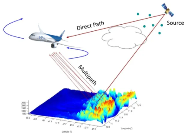
Figure 1: An example of multipath reflected by the ground which distorts the direct signal transmitted by the satellite.

the position delivered to user. This is the main motivation for its detection and mitigation. Multipath is defined as one or more indirect replicas of signals from satellites arriving at a receiver’s antenna from a satellite as shown for example in Figure1 for the case of an aircraft.

To address the problem of multipath detection, we propose a solution using raw data from the correlator output represented as a tensor of images from doppler and code delay offsets. We then use a CNN to automati-cally extract the features and a binary multipath classifier at the last layers of the network.

To assess the performance of our detector we run comparison experiments with another machine learning based method using a predefined feature construction procedure and a Support Vector Machine (SVM) clas-sifier [3].

The article is structured as follows. First, we review the related research done on the subject. Then we

describe the GNSS correlation process and the CNN concept. Thereafter, the data generation pipeline is de-tailed. The experiment setup is subsequently described and finally the results are discussed.

II. RELATED RESEARCH

A. GNSS multipath detection and mitigation

Two main approaches have been proposed in the literature, frequency-domain or time domain processing [4]. Among frequency-based approaches we can refer for example to the ones using the Fast Fourier Transform (FFT) [5], or the wavelet decomposition [6], [7]. How-ever, according to [4], these methods can unintentionally rule out other coexisting signals of interest. In the time-domain methods we can cite the Carrier Smoothing Filter (CSF) [8], [9] and the stacking technique in the case of static receiver [10]. These methods also tend to remove coexisting useful signals and their performance depends on the rate of the data flow.

The multipath mitigation can be done at the hardware level as well as the software level. At the hardware level, the use of high quality antenna arrays can be efficient for detecting and mitigating multipath [11]. They can also be used for estimating parameters of multipath. Alter-natively, the multipath can be mitigated at the software level of the receiver either in acquisition or in tracking loops. As the GNSS receiver has to track the direct signal contaminated by delayed reflections, several multipath mitigation methods based on the narrow correlator Delay Lock Loop (DLL) were listed in [12]. They include the strobe correlator [13], the early-late-slope technique [14], the double-delta correlator [15] and the multipath intensive delay lock loop [16]. On the other hand, a statistical approach based on the maximum likelihood principle [17] or the Bayesian technique [18] can be used.

In the case of Non-Line-of-Sight (NLOS) effect, mul-tipath can be hardly mitigated by these approaches. To overcome these limits, [12] proposes to use a Gener-alized Likelihood Ratio Test (GLRT) [19] and also a Marginalized Likelihood Ratio Test (MLRT) [20], for fault detection and diagnosis.

To avoid the limitations of these classical signal pro-cessing methods we consider the application of Machine Learning techniques [21], [22] to this multipath issue in GNSS.

B. Machine learning application in GNSS

The use of machine learning to facilitate the error mitigation and localization started from the early 2000s. In [1], the authors proposed method for multipath effect mitigation using a hybrid neural network architecture

based on multilayer perceptron for Law Earth Orbit (LEO) satellites. Otherwise, [4] treats the case of multi-path mitigation using a Support Vector Regression (SVR) model. Here, the author integrates kernel support vector regressor with geometrical features to deal with the code multipath error prediction on ground fixed GPS stations. Subsequent works were dedicated to the selection of different types of the relevant features to detect and mitigate multipath in their application. Examples of such work can be seen in [3] and [23] for NLOS multipath detection where the features are directly extracted from correlator output. In [24], the authors give the detailed description of CNNs and their application in the problem of carrier-phase multipath detection. In this work, the feature map was extracted from multivariable time series from the end of signal processing stage using a 1D convolutional layers.

Deep learning models in GNSS systems were also used for the problem of spoofing attack detection in GNSS receiver [25]. In this work, early-late phase, delta and signal level are the three main features extracted from the correlation output of the tracking loop. Using these features, spoofing detection is carried out using Deep Neural Networks (DNN) with fully-connected lay-ers within short detection time.

CNN have been used also for GNSS integration with misalignement detection of Inertial Navigation System (INS) [26]. The CNN was trained to detect the optical flow from smartphone camera to estimate the angle difference from moving direction to the inertial sensor. It allows to represent the distribution of objects moving on different images for misalignement calculation.

Our proposed method also uses a CNN to automat-ically extract relevant feature maps from the GNSS correlator output. Input data are represented in the form of 3D tensors in time-frequency domain. We discuss in details this idea in the next sections.

III. METHODOLOGY

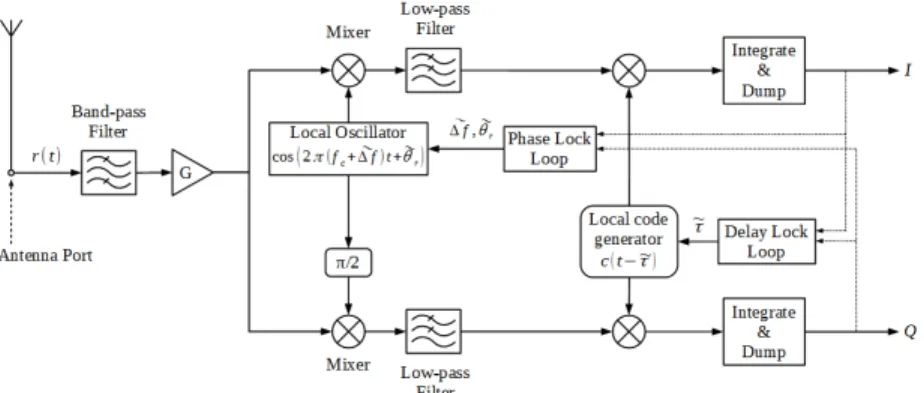
A. GNSS receiver architecture and signal processing In this section we will briefly present the model of GNSS correlator output. In this work, we consider the simplified model of signal at the antenna port, as can be seen in Figure2, which can be represented as:

r(t) = s(t) + b(t)

The desired signal s(t) is modeled as follows [27]: s(t) =

√

2CD(t − τ )c(t − τ ) cos(2π(fc+ ∆f )t + θr)

where

• D(t) is the navigation message;

• τ is the propagation delay;

• c(t) is the Pseudo-Random Noise (PRN) code

se-quence, corresponding to a specific satellite;

• fc is the carrier frequency; • ∆f is the doppler offset • θr is the carrier phase.

In this simplified model, we have taken the following hypothesis:

• The D(t) and c(t) terms are not distorted by

propagation;

• The propagation delay τ and Doppler offset ∆f are

constant;

• The propagation delay τ and carrier phase θr are

supposed to be independent.

The model of noise is considered to be the Additive White Gaussian Noise (AWGN), limited in frequency by the bandwidth of RF front-end. Indeed, it is the model of the noise as seen at the input of the RF front-end stage transfered to the antenna output. The noise term b(t) can be replaced by its Rice representation [28] as follows:

b(t) = ni(t)cos(2πflot + θr) − nq(t)sin(2πflot + θr)

where

• b(t) ∼ N (0, N0 Brf), AWGN, white at least on the

band of RF front-end;

• nq(t) ∼ N (0, N0 Brf) and nq(t) ∼ N (0, N0 Brf)

are AWGN on the bandwidth Bbb= Brf

2 ;

• N0₂ is the double sided noise Power Spectral

Den-sity (PSD);

• Brf is the RF front-end bandwidth.

The aim of the receiver is to estimate the propagation delay τ for each satellite in view so as to calculate the user position according to a trilateration principle. ∆f and θr are nuisance parameters which have to be

estimated too.

The first step in the signal processing chain is the mul-tiplication of the incoming signal by two local replicas in quadrature of the carrier signal. This operation splits the signal into two channels: in-phase (I) and quadrature (Q) as follows:

pcos(t) = r(t) · cos(2π(fc+ ˜∆f )t + ˜θr)

psin(t) = −r(t) · sin(2π(fc+ ˜∆f )t + ˜θr)

where ˜∆f is the local estimate of the doppler offset ∆f and ˜θr is the local estimate of the initial phase θr of the

carrier signal. The two components pcos(t) and psin(t)

are then low-pass filtered to remove the high-frequency terms in 2fc.

Then, the two channels are correlated with a locally generated PRN code sequence. This correlation opera-tion is performed by the means of a multiplier followed by the Integrate-and-Dump (I&D) stage. The latter is parametrized by the coherent integration time Ti.

Finally, a model of the signal available at the output of the I&D stage, which is the correlator output, is [29]:

I = M cos(π(∆f − ˜∆f )Ti+ (θr− ˜θr)) × sinc(π(∆f − ˜∆f )Ti) + nI (1) Q = −M sin(π(∆f − ˜∆f )Ti+ (θr− ˜θr)) × sinc(π(∆f − ˜∆f )Ti) + nQ (2) where • M = DTi 2 q C 2K(˜τ − τ )

• D is the value of the bit of the navigation message, which remains constant over the coherent integra-tion time Ti;

• K(˜τ −τ ) is the auto-correlation function of the PRN code in ˜τ − τ ;

• τ is the local estimate of the propagation delay τ ,˜

hence ˜τ − τ is the propagation delay estimation error;

• ∆f − ˜∆f is the doppler estimation error; • θr− ˜θr is the phase estimation error;

• nI(t) ∼ N (0,N0 T₁₆i) and nQ(t) ∼ N (0,N0 T₁₆i) are

two independent and identically distributed white noise components;

It is worth noting that the I and Q components of the correlator output are being produced each Ti.

B. CNN general description

In this part, we will describe the motivation behind the application of CNN in the GNSS correlation output data processing. We try to take advantage of the fact that in the case of structured and hierarchical data CNNs are capable to efficiently extract feature maps. The correlator output signal can be seen as a structured and hierarchical data.

Indeed, the correlator output double-channel data can be easily represented in the form of a 3D tensor like multi-channel "image" and correlator output values can be translated to the predictive model as the intensity of pixels in both I and Q channels.

The definition and principles of CNN are described in details in [30], [31]. According to [31], convolution leverages three important ideas that can help improve a machine learning system: sparse interactions, parameter sharing and equivariant representations. Unlike the clas-sical DNN where every output unit interacts with every

Figure 2: Typical model of the signal correlation chain of a GNSS receiver input unit, through matrix multiplication of parameters,

CNN typically promotes sparse interactions. This also means that fewer parameters need to be stored, which reduces the memory requirements of the model and im-proves its statistical efficiency and decreases its operation complexity.

The data used with CNNs usually consists of several channels, each channel being the observation of a dif-ferent quantity in difdif-ferent axis scales. One of such data type is a color image data where each channel contains the color of pixels. The convolution kernel moves over both the horizontal and the vertical axes of the image, conferring translation equivariance in both directions.

A typical CNN architecture is composed of the fol-lowing basic elements as it can be seen in Figure3.

• Convolutional layer: A convolutional filter (kernel)

within convolutional layers provides a compressed representation of input data. With convolutional filters computed using CNN, convolutional layers can extract features from input data. Each filter is composed of weights that can be either predefined or trained during learning process, which is the case in our study.

• Pooling layer: The convolved features are subsam-pled by a specific factor in the subsampling layer. The role of a subsampling layer is to reduce the variance of convolved data so that the value of a particular feature over a region of an input layer can be computed and merged together.

• Activation function: Following several convolu-tional and pooling layers, the high-level reasoning in the neural network is performed via fully con-nected layers. Neurons in a fully concon-nected layer have full connections to all activation in the previ-ous layer. Fully connected layers eventually convert the 2D feature maps into a 1D feature vector. The derived vector either could be fed forward into

a certain number of categories for classification or could be considered as a feature for further processing.

The specific architecture and setup of our CNN model dedicated to the multipath detection at the correlator output will be described in the SectionV.

IV. GNSS DATA GENERATION AND LABELLING

A. Main signal generation

In order to test our prediction models, an artificial signal generator was developed. The data is generated in the form of two matrices, one for each of the I and Q channels, according to equations (1) and (2). As a GNSS receiver is built to estimate the doppler and propagation delay, the axes of these matrices were defined in doppler estimation error ∆f − ˜∆f and code delay estimation error τ − ˜τ . Phase estimation is represented implicitly by I and Q components of the correlator output. The output data corresponding to this main signal can be parametrized as follows:

• Coherent integration time Ti in ms; • Carrier-to-noise ratio C/N0 in dBHz.

An illustration of the output of our generator in terms of I(t)2_{+ Q(t)}2 _{is given in Figure4 for two different}

integration times.

B. Multipath generation

If a multipath signal is received in addition to the main signal, as the signal processing chain is linear, we can then consider that the correlator output is the sum of the correlator output of the main signal plus the one due to the multipath:

I0 = I + IM P(αM P, ∆τM P, ∆fM P, ∆θM P)

Q0 = Q + QM P(αM P, ∆τM P, ∆fM P, ∆θM P)

Figure 3: CNN structure and main elements example [32]

Figure 4: Synthetic correlator output visualization for Tint= 1 ms (left) and Tint= 20 ms (left)

• ∆τM P > 0 is the code delay in excess to the main

signal delay τ ;

• ∆fM P is the difference between the doppler offset

of the main signal and the multipath;

• ∆θM P is the difference between the phase of the

main signal and the multipath;

• αM P is the multipath attenuation coefficient in

comparison to the main path.

The generation range for the code delay estimation error is set to [0, 2] chips, where one chip is the duration of one bit of the PRN code sequence. This is because out-side of this interval the correlation value is negligible, so the multipath effect is annihilated. Regarding the doppler offset estimation error range, it is defined as ±_T1

i, the

width of the main lobe of the sinc function in (1) and (2). We have considered that outside of this interval the side lobes of the sinc function attenuate enough the multipath component. With no a priori information, the phase estimation error range was set to [0, 2π]. The multipath attenuation was ranged in [0.5, 0.9] so as to consider the most powerful, hence harmful, multipath.

C. Training Dataset construction

Also it needs to be noticed that to be represented in the form of 3D tensors, the processed signal needs to be discretized by a predefined number of correlator outputs depending on the given GNSS receiver con-figuration. So to cover all such possible configurations we have used the following set of discretization levels: N ∈ {4, 6, 8, 10, 20, 30, 40} points in each range τ − ˜τ and ∆f − ˜∆f . That is to say the number of correlator outputs is N2_.

As the multipath effect cannot be considered as a rare event (for example in urban environment), the simulated dataset was generated so that it is well balanced between two classes:

• Category A: represents normal signal with no reflec-tions (data from Category A is labelled as direct-signal only data).

• Category B: simulates signals with a single multi-path effect which can include doppler, code delay or phase offsets (data from Category B is labelled as multipath event).

See [33] for a public release of our generator code. V. EXPERIMENT

A. Selected CNN architecture

The architecture and training parameters of the de-signed CNN are shown in TableI.

The feature extraction part of the CNN consists of 4 convolutional blocks with 2 convolutional layers in each block and pooling layers at the end of each block. For example, consider a correlator output image cropped up to discretization size N = 40 × 40 × 2 that is passed through the network. The first convolutional layer from the first block (conv1-1) is a feature map with a size 40 × 40 × 16, where the dimensions indicates height, width and number of channels. This layer is generated

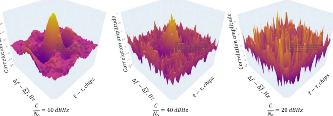
Figure 5: Synthetic correlator output visualization for I-channel for different values of carrier-to-noise ratio Table I: CNN hyperparameters

Nb Layers 4 Blocks of 2 Conv layers Loss LogLoss Optimizer Adam Learning rate 10−3_...10−4

Batch size 32 Nb epochs 30

by the convolutional operation of 16 filters. Each filter corresponds to a channel of the feature map, respectively. By using maxpooling operation of pooling size 2×2 and stride size 2 × 2, the dimensions feature of the map are reduced to 20×20×16 in the second convolutional layer of the first block (conv1-2).

The decision to use the convolutional layers assembled in blocks was made to avoid the use of large-sized kernels (for example 7 × 7 or 5 × 5) with multiple 3 × 3 kernel-sized filters one after another. It is especially true for the case of scalable image discretization size which can vary in wide range from 40 to 300 pixels. This kind of architecture was succesfully applied in the VGG family of convolutional neural networks [34] on the ImageNet dataset of over 14 million images belonging to 1000 classes.Thus VGGNet-like architectures can be considered as a baseline feature extractors.

The classifier part of the CNN consists of two fully-connected layers of size 1152 × 1 and 256 × 1 with the sigmoid output activation function.

B. Benchmark model

The performance of the proposed method is compared to those described in [3]. The method is based on the Support Vector Mashine (SVM) approach. Reported results show that 87% of the signals were correctly dis-criminated (results depend on the number of correlation data points used). Since the method also collects data from the output of the correlator block, it follows the

Table II: SVM hyperparameters

Kernel 4 RBF (Gaussian) Cross Val 3 Folds Normalization Standard Scale

same process as our technique.

We have implemented the same feature extraction pipeline and used the same SVM classifier hyperparam-eters [35], [36] on our synthetic dataset to compare the efficiency of the proposed CNN algorithm (referred as MultipathCNN in the following). To obtain the correla-tion shape we also use 13 correlator outputs.

As in [3], the following features were extracted:

• Number of local maxima of the correlation outputs per period F2 =

Nlocal−maxima

∆t ; where ∆t is the

correlation interval taken equal to coherent integra-tion period.

• Distribution of the delay of the maximum corre-lation output F3 = _M1 P

M

i=1(ti−max − ¯t)2 where

ti−max is the code delay of the maximum

correla-tion output, ¯t is the mean of the code delay, and M is the number of correlator output samples. In [3], the authors have also used a signal strength vs. elevation angle feature (referred as F1) that is not taken

into account here as we have not introduced the physical context of experiments (receiver’s speed, satellite con-stellation) since the generated dataset is synthetic. Thus, we have made the choice to not use the feature F1 as

opposed to [3].

Table IIreports the SVM hyperparameters that were used during the experiment.

C. Experimental setup

The strategy of experiments was designed for the cases of coherent integration time of Ti ∈ {1, 20} ms. The

synchronisation with the navigation message, the largest one being used after synchronisation. For each of two values of integration time we have conducted two types of tests:

• Tests on various discretization levels N ;

• Tests on models benchmark comparison.

It is worth noting that for both types of test above, we make comparisons for several values of the following parameters:

• ∆θM P = {0, 45, 90, 180}◦; • C/N0 ∈ {20, 30, 40, 50, 60} dBHz; • αM P ∼ U ([0.5, 0.9]).

A variation of the I component with respect to C/N0 is illustrated in Figure5.

1) Type 1. Tests on various discretization levels During this stage we have conducted tests of our MultipathCNN algorithm on discretization levels N ∈ {4, 6, 8, 10, 20, 30, 40} to estimate the optimal value of discretization. To model the multipath effect we have picked randomly the doppler offset uniformly as ∆fM P ∼ U ([0, 1000]) Hz and the code delay offset

as ∆τM P ∼ U ([0.1...0.8]) chips separately for each

discretization level.

2) Type 2. Test on models benchmarks comparison In this stage, we have performed the test to compare the performance of our MultipathCNN model with the reference SVM model. We have chosen fixed discretiza-tion level of 10 correlator outputs to be closer to the case of SVM (with its 13 correlator outputs). We have also picked randomly and uniformly the doppler and the code delay offsets in the same range as in the first type of experiments with simultaneous variation of these parameter.

D. Results tables and figures description

In order to evaluate the performance of multipath detectors, the two models were applied directly to the synthetic dataset which was varying in different con-figurations listed above. We compare our results with state-of-the-art method using an accuracy metric.

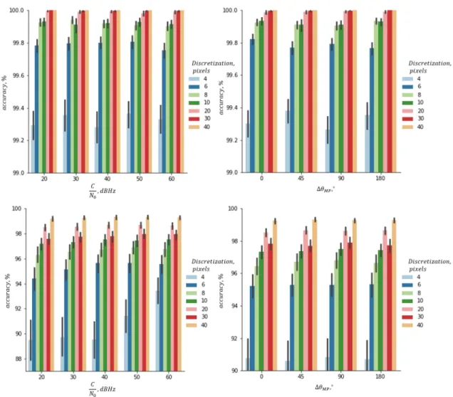
In Figure 6 we provide the barplots which represent the accuracies of the model MultipathCNN on prediction of multipath. These results are averaged over 20 runs of the test of type 1 described earlier. Here the results are represented as function of different C/N0 values and multipath phase offsets ∆θM P. For each of these

param-eters the results are also grouped by the discretization level N .

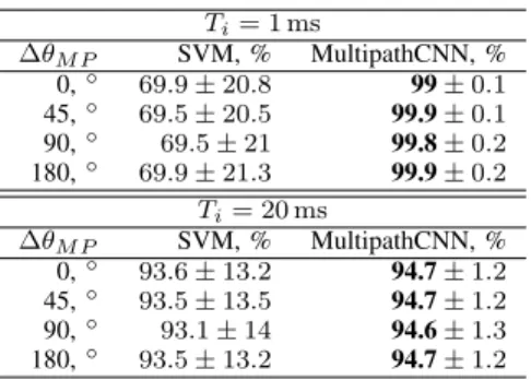
In tables III and IV we provide also the values of accuracy averaged over 20 runs for different levels of C/N0 and ∆θM P. These results correspond to the tests

Table III: Average model performance on benchmark test as the function of phase offset

Ti= 1 ms ∆θM P SVM, % MultipathCNN, % 0,◦ 69.9 ± 20.8 99 ± 0.1 45,◦ 69.5 ± 20.5 99.9 ± 0.1 90,◦ 69.5 ± 21 99.8 ± 0.2 180,◦ 69.9 ± 21.3 99.9 ± 0.2 Ti= 20 ms ∆θM P SVM, % MultipathCNN, % 0,◦ 93.6 ± 13.2 94.7 ± 1.2 45,◦ 93.5 ± 13.5 94.7 ± 1.2 90,◦ 93.1 ± 14 94.6 ± 1.3 180,◦ 93.5 ± 13.2 94.7 ± 1.2

Table IV: Average model performance on benchmark test as the function of C/N0 Ti= 1 ms C/N0 , dBHz SVM, % MultipathCNN, % 20 62.2 ± 14.1 99.8 ± 0.2 30 73.8 ± 23.9 99.9 ± 0.1 40 71.1 ± 21.3 99.9 ± 0.2 50 70.7 ± 21 99.8 ± 0.2 60 70.8 ± 21.1 99.8 ± 0.2 Ti= 20 ms C/N0 , dBHz SVM, % MultipathCNN, % 20 67.5 ± 7.7 94.3 ± 1.2 30 99.6 ± 1 94.4 ± 1.1 40 100 ± 1.1 94.8 ± 1.2 50 100 ± 1.1 94.8 ± 1.1 60 100 ± 1 95 ± 1.2

of type 2 described above.

E. Discussion on results

1) Tests on various discretization level

As it can be seen in Figure 6, the reduction of discretization level up to 4, 6 discretization levels leads in average to the reduction of model accuracy by 8% and degrades slightly the variance of other MultipathCNN model accuracy. It can also be seen that for the case of integration time of 20 ms, the models with 4 and 6 correlator outputs become sensitive to the C/N0 vari-ation. However, for the case of integration time of 1 ms, C/N0 variation has almost no significant influence on the models performance. Regarding the influence of the phase offset, the sole case of ∆θ = 90◦ shows the degradation in the model metrics by at most 0.5%.

As our final objective in the future is to integrate the multipath detector in the GNSS receiver, we need to find the minimum number of correlator outputs N keeping an accuracy high enough to detect the multipath effect. Taking into account the test results, N ∈ {8, 10} seems a reasonable value which is insensitive to the

Figure 6: Accuracy in % averaged over 20 runs of MultipathCNN for various levels of discretization for two integration times: 1 ms (up) and 20ms (bottom)

level of noise in the signal. A discretization level of N = 8 gives us 64 correlator outputs which seems to be feasible in comparison to [37] approach which proposes 48 correlator outputs.

2) Tests on models benchmark comparison

The results shows that our proposed method outper-forms the SVM on the synthetic GNSS dataset. De-pending on the coherent integration time, the results are represented as follows:

• For the case of integration time of Ti = 1 ms,

our model outperforms the SVM on every value of C/N0 and phase offset.

• For the case of integration time of Ti= 20 ms and

the values of C/N0 ∈ [30, 60] dBHz our model shows 5% less accuracy than the benchmark, but outperforms it for low C/N0 value.

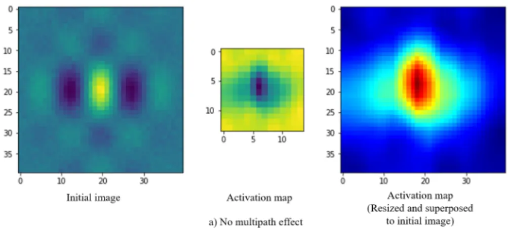
We believe that these performance results of the Mul-tipathCNN are due to the fact that the CNN is able to catch the geometrical dependencies in the data. To demonstrate this property, we have used the visualized heatmaps of class activation at the last convolutional layer. In the example on Figure 3 it corresponds to the output of the third convolutional layer (C3). This can help to understand which part of an image led a CNN to its final classification decision. It can be seen on Figures 7 and 8, where the activation map of the last convolutional layer of MultipathCNN shows the distortion of the central zone of correlation peak for the cases without multipath and with multipath respectively. Thus, we see that MultipathCNN is capable to build a discriminant for multipath that human could not conceive a priori. Concerning the computational cost, we expect

the run-time to be tractable with an optimal architecture, also considering that in prediction mode there is only a forward pass and that computation can be distributed on several CPU/GPUs.

VI. CONCLUSION AND FURTHER WORK

In this study a CNN based multipath detection method has been proposed to detect multipath in the GPS L1 C/A correlator output stage. The proposed method has been validated with synthetic GPS data generator. The performance of the detector has been compared to SVM based multipath detector. The results have shown that MultipathCNN performs better than the compared method especially when the C/N0 degrades.

The proposed algorithm should now be validated against ground truth, that is real physical signal.

ACKNOWLEDGEMENTS

This project has been partly funded by the SESAR Joint Undertaking under the European Union’s Horizon 2020 research and innovation programme under grant agreement No 783287. The opinions expressed herein reflect the authors’ view only. Under no circumstances shall the SESAR Joint Undertaking be responsible for any use that may be made of the information contained herein.

REFERENCES

[1] W. Vigneau, O. Nouvel, M. Manzano-Jurado, C. Sanz, H. Ab-dulkader, D. Roviras, J. M. Juan, and P. Holsters, “Neural networks algorithms prototyping to mitigate GNSS multipath for LEO positioning applications,” in Proceedings of the 19th International Technical Meeting of the Satellite Division of The Institute of Navigation (ION GNSS 2006), Sep. 2006, pp. 1752– 1762.

[2] P. D. Groves, Z. Jiang, L. Wang, and M. Ziebart, “Intelligent urban positioning, shadow matching and non-line-of-sight signal detection,” in 2012 6th ESA Workshop on Satellite Navigation Technologies (Navitec 2012) European Workshop on GNSS Sig-nals and Signal Processing, Dec 2012, pp. 1–8.

[3] T. Suzuki, Y. Nakano, and Y. Aman, “NLOS multipath detection by using machine learning in urban environments,” in 30th International Technical Meeting of the Satellite Division of the Institute of Navigation, ION GNSS 2017, vol. 6. Institute of Navigation, Jan. 2017, pp. 3958–3967.

[4] Q.-H. Phan, S.-L. Tan, I. V. McLoughlin, and D.-L. Vu, “A unified framework for GPS code and carrier-phase multipath mitigation using support vector regression,” Adv. Artificial Neural Systems, vol. 2013, pp. 240 564:1–240 564:14, 2013.

[5] Yujie Zhang and C. Bartone, “Multipath mitigation in the fre-quency domain,” in PLANS 2004. Position Location and Navi-gation Symposium (IEEE Cat. No.04CH37556), April 2004, pp. 486–495.

[6] M. Elhabiby, A. El-Ghazouly, and N. El-Sheimy, “A new wavelet-based multipath mitigation technique,” in Proceedings of the 21st International Technical Meeting of the Satellite Division of The Institute of Navigation (ION GNSS 2008), vol. 2, Sep. 2008, pp. 625–631.

[7] Y. Zhang and C. Bartone, “Real-time multipath mitigation with WaveSmoothTM technique using wavelets,” in Proceedings of the

17th International Technical Meeting of the Satellite Division of The Institute of Navigation (ION GNSS 2004), Sep. 2004, pp. 1181–1194.

[8] P. Y. Hwang, G. A. Mcgraw, and J. R. Bader, “Enhanced differential GPS carrier-smoothed code processing using dual-frequency measurements,” Navigation, vol. 46, no. 2, pp. 127–137, jun 1999. [Online]. Available: https://doi.org/10. 1002%2Fj.2161-4296.1999.tb02401.x

[9] P. Misra and P. Enge, Global Positioning System: Signals, Measurements, and Performance. Ganga-Jamuna Press, 2011. [Online]. Available: https://books.google.fr/books?id= 5WJOywAACAAJ

[10] P. Axelrad, K. M. Larson, and B. A. Jones, “Use of the correct satellite repeat period to characterize and reduce site-specific multipath errors,” in Proceedings of the 18th International Technical Meeting of the Satellite Division of The Institute of Navigation (ION GNSS 2005), Sep. 2005, pp. 2638–2648. [11] Z. Jiang and P. D. Groves, “NLOS GPS signal detection using

a dual-polarisation antenna,” GPS Solutions, vol. 18, pp. 15–26, 2012.

[12] C. Cheng, J.-Y. Tourneret, Q. Pan, and V. Calmettes, “Detecting, estimating and correcting multipath biases affecting GNSS sig-nals using a marginalized likelihood ratio-based method,” Signal Processing, vol. 118, Jul. 2015.

[13] L. J. Garin, F. van Diggelen, and J.-M. Rousseau, “Strobe & edge correlator multipath mitigation for code,” in Proceedings of the 9th International Technical Meeting of the Satellite Division of The Institute of Navigation (ION GPS 1996), Sep. 1996, pp. 657–664.

[14] B. Townsend and P. Fenton, “A practical approach to the reduc-tion of pseudorange multipath errors in a L1 GPS receiver,” in Proceedings of ION GPS-94, 1994, pp. 143–148.

[15] G. A. Mcgraw and M. S. Braasch, “GNSS multipath mitigation using gated and high resolution correlator concepts,” in Proceed-ings of the 1999 National Technical Meeting of The Institute of Navigation, Jan. 1999, pp. 333–342.

[16] N. Jardak, A. Vervisch-Picois, and N. Samama, “Multipath in-sensitive delay lock loop in GNSS receivers,” IEEE Transactions on Aerospace and Electronic Systems, vol. 47, pp. 2590–2609, 2011.

[17] R. D. J. van Nee, J. Siereveld, P. C. Fenton, and B. R. Townsend, “The multipath estimating delay lock loop: approaching theo-retical accuracy limits,” in Proceedings of 1994 IEEE Position, Location and Navigation Symposium - PLANS’94, April 1994, pp. 246–251.

[18] S. M. F. S. Dardin, V. Calmettes, B. Priot, and J.-Y. Tourneret, “Design of an adaptive vector-tracking loop for reliable po-sitioning in harsh environment,” in Proceedings of the 26th International Technical Meeting of the Satellite Division of The Institute of Navigation (ION GNSS+ 2013), Sep. 2013, pp. 3548– 3559.

[19] A. Willsky and H. Jones, “A generalized likelihood ratio approach to the detection and estimation of jumps in linear systems,” IEEE Transactions on Automatic Control, vol. 21, no. 1, pp. 108–112, February 1976.

[20] F. Gustafsson, “The marginalized likelihood ratio test for detect-ing abrupt changes,” IEEE Transactions on Automatic Control, vol. 41, no. 1, pp. 66–78, Jan 1996.

[21] A. Mueller and S. Guido, Machine learning avec Python. O’Reilly Media, Inc., 2018. [Online]. Available: https://books. google.fr/books?id=7TBvDwAAQBAJ

[22] T. Hastie, R. Tibshirani, and J. Friedman, The Elements of Statistical Learning, ser. Springer Series in Statistics. New York, NY, USA: Springer New York Inc., 2001.

[23] L. Hsu, “GNSS multipath detection using a machine learning approach,” in 2017 IEEE 20th International Conference on Intelligent Transportation Systems (ITSC), Oct 2017, pp. 1–6.

Figure 7: Activation map from the last convolutional layer of the MultipathCNN for the case without multipath in the tensor with discretization 40 × 40 for integration time Ti= 1 ms

Figure 8: Activation map from the last convolutional layer of the MultipathCNN for the case with multipath in the tensor with discretization 40 × 40 for integration time Ti= 1 ms

[24] Y. Quan, L. Lau, G. W. Roberts, X. Meng, and C. Zhang, “Convolutional neural network based multipath detection method for static and kinematic GPS high precision positioning,” Remote Sensing, vol. 10, p. 2052, 2018.

[25] E. Shafiee, M. Mosavi, and M. Moazedi, “Detection of spoofing attack using machine learning based on multi-layer neural net-work in single-frequency GPS receivers,” Journal of Navigation, vol. 71, pp. 1–20, 08 2017.

[26] T. Su and H.-W. Chang, “Computer vision combined with convo-lutional neural network aid GNSS/INS integration for misalign-ment estimation of portable navigation,” in 30th International Technical Meeting of the Satellite Division of the Institute of Navigation, ION GNSS 2017, vol. 1. United States: Institute of Navigation, 1 2017, pp. 611–621.

[27] E. Kaplan and C. Hegarty, Understanding GPS: Principles and Applications, ser. Artech House mobile communications series. Artech House, 2005. [Online]. Available: https: //books.google.fr/books?id=-sPXPuOW7ggC

[28] S. O. Rice, “Envelopes of narrow-band signals,” Proceedings of the IEEE, vol. 70, no. 7, pp. 692–699, July 1982.

[29] J.-H. Won and T. Pany, Springer Handbook of Global Navigation Satellite Systems, 1st ed. Springer International Publishing, 2017, ch. Signal Processing, pp. 401–442.

[30] F. Chollet, Deep Learning with Python. Manning, Nov. 2017. [31] I. Goodfellow, Y. Bengio, and A. Courville, Deep Learning.

MIT Press, 2016, book in preparation for MIT Press. [Online]. Available:http://www.deeplearningbook.org

[32] A. Voulodimos, N. Doulamis, A. Doulamis, and E. Protopa-padakis, “Deep learning for computer vision: A brief review,” Computational Intelligence and Neuroscience, vol. 2018, pp. 1– 13, 02 2018.

[33] E. Munin, A. Blais, and N. Couellan, “Convolutional neural network for multipath detection in GNSS receivers,” https://github.com/EvgeniiMunin/gnss_signal_generator. [On-line]. Available: https://github.com/EvgeniiMunin/gnss_signal_ generator

[34] K. Simonyan and A. Zisserman, “Very deep convolutional networks for large-scale image recognition,” CoRR, vol. abs/1409.1556, 2014. [Online]. Available: http://arxiv.org/abs/ 1409.1556

[35] V. N. Vapnik, Statistical Learning Theory. Wiley-Interscience, 1998.

[36] B. Scholkopf and A. J. Smola, Learning with Kernels: Sup-port Vector Machines, Regularization, Optimization, and Beyond. Cambridge, MA, USA: MIT Press, 2001.

[37] A. M. Mitelman, R. E. Phelts, D. Akos, S. Pullen, and P. Enge, “A real-time signal quality monitor for GPS augmentation systems,” in Proceedings of the 13th International Technical Meeting of the Satellite Division of The Institute of Navigation (ION GPS 2000), Sep. 2000, pp. 862–871.