HAL Id: hal-01580275
https://hal.archives-ouvertes.fr/hal-01580275v3
Submitted on 11 Oct 2017
HAL is a multi-disciplinary open access
archive for the deposit and dissemination of
sci-entific research documents, whether they are
pub-lished or not. The documents may come from
teaching and research institutions in France or
abroad, or from public or private research centers.
L’archive ouverte pluridisciplinaire HAL, est
destinée au dépôt et à la diffusion de documents
scientifiques de niveau recherche, publiés ou non,
émanant des établissements d’enseignement et de
recherche français ou étrangers, des laboratoires
publics ou privés.
Probabilistic Analysis of Counting Protocols in
Large-scale Asynchronous and Anonymous Systems
Yves Mocquard, Bruno Sericola, Emmanuelle Anceaume
To cite this version:
Yves Mocquard, Bruno Sericola, Emmanuelle Anceaume. Probabilistic Analysis of Counting
Pro-tocols in Large-scale Asynchronous and Anonymous Systems. 2017 IEEE 16th International
Sym-posium on Network Computing and Applications (NCA), Oct 2017, Cambridge, United States.
�10.1109/nca.2017.8171371�. �hal-01580275v3�
Probabilistic Analysis of Counting Protocols in
Large-scale Asynchronous and Anonymous Systems
Yves Mocquard
Universit´e de Rennes 1/IRISA,Bruno Sericola
INRIA Rennes - Bretagne Atlantique, [email protected]
Emmanuelle Anceaume
CNRS/IRISA, [email protected]Abstract—We consider a large system populated by n anony-mous nodes that communicate through asynchronous and pair-wise interactions. The aim of these interactions is for each node to converge toward a global property of the system, that depends on the initial state of each node. In this paper we focus on both the counting and proportion problems. We show that for any δ ∈ (0, 1), the number of interactions needed per node to converge is O(ln(n/δ)) with probability at least 1− δ. We also prove that each node can determine, with any high probability, the proportion of nodes that initially started in a given state without knowing the number of nodes in the system. This work provides a precise analysis of the convergence bounds, and shows that using the 4-norm is very effective to derive useful bounds. Keywords Large scale anonymous and asynchronous system; Counting problem; Proportion problem; Markov chain; Prob-abilistic analysis.
I. INTRODUCTION
This paper focuses on the analysis of counting problems in a model in which nodes are identically programmed, with no identity, and they progress in their computation through random pairwise interactions. As motivated by Aspnes [3], the objective of this model is to analyze the conditions under which nodes can converge to a state from which some global property of the system can be locally computed. A consider-able amount of work has been done so far to determine which properties can emerge from pairwise interactions between finite-state nodes, together with the derivation of lower bounds on the time and space needed to reach such properties (e.g., [1], [2], [4], [6], [9]). In this work, we are primarily interested in counting problems. Briefly, each node starts independently of each other in one of two input states, say A and B, and the objective for each node is to eventually reach a state from which it can derive with any high probability the exact difference between the number of nodes that started their execution with A, denoted by nA in the following, and the
number of nodes that started their execution with B, denoted by nB.
The main contribution of this work is an analysis of the time for all the nodes of the system to converge to nA− nB
with any probability fixed in advance. This analysis improves upon the one obtained by Mocquard et al. [7] thanks to the tools used to derive this convergence time. In [7], the 2-norm of the difference between the vector of states of the nodes and the
This work was partially funded by the French ANR project SocioPlug (ANR-13-INFR-0003), and by the DeSceNt project granted by the Labex CominLabs excellence laboratory (ANR-10-LABX-07-01).
limiting distribution of these states is analyzed. In the present paper, we use the 4-norm, and we precisely characterize the conditions under which the 4-norm gives tighter bounds with respect to the the 2-norm. To the best of our knowledge, such an analysis has never been achieved before.
In the remaining of the paper we define in Section II both the counting problem and the proportion one, and examine in Section IV the different works that have tackled those problems. In Section III we formally present the model in which this work has been done. We present in Section V the protocols run by the nodes to solve both problems. After the statement of preliminary results in Section VI, we then study in Section VII the moments and the distribution of the difference between the random vector of all agents’ values and the limiting distribution of these values. In Section VIII we analyze their bounds and asymptotic behavior when the number n of nodes goes to infinity. The accuracy of our analytic study has been illustrated through numerous simulations whose main results are presented in Section IX.
II. THE ADDRESSED PROBLEMS
We consider a set of n agents, interconnected by a complete graph, that asynchronously start their execution in one of two distinct states A and B. Let nA (resp. nB) be the number of
agents whose initial state is A (resp. B), and let κ = nA−
nB. This paper addresses two related problems, the counting
problem and the proportion one, both defined as follows.
a) Counting problem.: A population protocol ran by all
the nodes of the system solves the counting problem in τ steps with probability at least 1− δ, for any δ ∈ (0, 1), if for any
t≥ τ, it holds that for any node i of the system, i is capable
of computing κ with probability at least 1− δ.
b) Proportion problem.: A population protocol ran by
all the nodes of the system solves the proportion problem in
τ steps with probability at least 1− δ, for any δ ∈ (0, 1), if
for any t ≥ τ, it holds that for any node i of the system, i is capable of computing nA/n with probability at least 1− δ,
without having access to the population size n.
III. MODEL ANDNOTATIONS
In this work we assume that a collection of nodes are connected by a complete graph and communicate through pairwise and asynchronous interactions. Initially, all the nodes start with an initial state represented by the symbol A or B, and upon interactions, update their local state according to the transaction function f . Interactions between nodes are random:
at each discrete time, any two agents are randomly selected to interact. The notion of time in population protocols refers to as the successive steps at which interactions occur, while the parallel time refers to as the total number of interactions averaged by n, see Aspnes et al. [3]. Note that nodes do not maintain nor use identifiers, however for ease of presentation, they are numbered 1, 2, . . . , n.
We will denote by Ct(i) the state of node i at time t. The configuration of the system at time t is the state of each node at time t and is denoted by Ct= (C
(1)
t , . . . , C
(n)
t ). We denote
by Xt the random pair of distinct nodes chosen at time t to
interact, and for every i, j = 1, . . . , n, with i ̸= j, we define
pi,j(t) =P{Xt= (i, j)}.
We suppose that the sequence {Xt, t ≥ 0} is a
se-quence of independent and identically distributed random variables. Since Ct is entirely determined by the values of
C0, X0, X1, . . . , Xt−1, this means in particular that the random
variables Xt and Ct are independent and that the stochastic
process C = {Ct, t ≥ 0} is a discrete-time homogeneous
Markov chain. Note that this Markov chain is very hard to analyze using classical Markov chains methods because its state space is quite complex. Nevertheless, as we will see, the simplicity of the transition function f allows us to get interesting results.
IV. RELATEDWORK
The closest problems to the one we address are the com-putation of the majority (see [4], [6], [2], [9], [1]). In this problem, all the agents start in one of two distinct states and they eventually converge to 1 if κ > 0 (i.e. nA> nB), and to 0
if κ≤ 0 (i.e. nA≤ nB). Draief and Vojnovic [4] and Mertzios
et al. [6] propose a four-state protocol that solves the majority problem with a convergence parallel time logarithmic in n but only in expectation. Moreover, the expected convergence time is infinite when nA and nB are close to each other (that is κ
approaches 0). Angluin et al.[2] and Perron et al. [9] propose a three-state protocol that converges with high probability after a convergence parallel time logarithmic in n but only if κ is large enough, i.e when |nA− nB| ≥
√
n log n. Alistarh
et al. [1] present a nice protocol based on an average-and-conquer method to solve the majority problem. The first type of interaction is close to the one used in this paper while the second one is used to diffuse the result of the computation to the agents that have not decided yet. Actually, to show their convergence time, they need to assume a large number of intermediate states because they need to prove that all the agents with maximum positive values and minimal negative values will have sufficiently enough time to halve their values. Note that in practice, their algorithm does not require more than n state to converge to the majority. Note that the protocol proposed by Jelasity et al. [5] computes the average of the initial values of the nodes, as done in the present paper, however, in their protocol nodes act synchronously. Finally in a previous work [7] we have presented a solution to the majority counting problem, whose originality was a proof of convergence based on tracking the euclidean distance between the vector of all agents’ states and the limiting distribution of these states. In a more recent work [8], we have provided an analysis which shows that when nodes can only manipulate integers, then our solution to both the counting problem and
the proportion one are optimal both in time and space. In the present paper, we tackle the case where nodes manipulate dyadic rational numbers, and we provide tighter bounds on the time needed for each node to converge to the sought result.
V. THECOUNTING ANDPROPORTIONPROTOCOLS
Initially, all the nodes i, 1 ≤ i ≤ n start with a symbol
A or B that provides their initial state C0(i). Let m be any
positive integer. We set
C0(i)= {
m if the initial local state is A
−m if the initial local state is B.
Interactions between nodes are orchestrated by a random scheduler: at each discrete time t≥ 0, any two indices i and
j are randomly chosen to interact with probability pi,j(t).
Note that the random scheduler is fair, meaning that any possible interaction cannot be avoided forever. Once chosen, the pair of nodes (i, j) interacts and both nodes update their respective state Ct(i) and Ct(j) by applying the following transition function f , leading to state Ct+1, given by
( Ct+1(i), Ct+1(j) ) = f ( Ct(i), Ct(j) ) = ( Ct(i)+ Ct(j) 2 , Ct(i)+ Ct(j) 2 ) (1) and Ct+1(h) = Ct(h) for h̸= i, j.
At any time t, and upon request from the application, any node
i of the system can provide its estimation of κ = nA− nB by
returning wi, defined as wi= ⌊ Ct(i)n m + 1 2 ⌋ .
We show in the following (see Corollary 7) that with any high probability, wi = κ for any node i in the system. Note
that the values taken by the variables Ct(i) belong to the set of dyadic numbers (the rational numbers whose denominator is a power of 2) of the interval [−m, m].
The proportion protocol uses the interaction function f defined in Relation (1), and the estimation of the proportion
nA/n is defined as
w′i=
Ct(i)+ m
2m .
Note that node i does not need to know the size n of the population to compute the proportion of nodes that started with symbol A. We show with Corollary 8 (shown in Section VII) that with any high probability and with any high precision,
wi′≈ nA/n for any node i in the system.
VI. PRELIMINARYRESULTS
The following Lemma states that the sum of the entries of vector Ctis constant.
We denote by ℓ the mean value of the sum of the entries of Ctand by L the row vector ofRn with all its entries equal
to ℓ, that is ℓ = 1 n n ∑ i=1 Ct(i) and L = (ℓ, . . . , ℓ).
For every d ∈ N \ {0} and x = (x1, . . . , xn)∈ Rn, we will
use the d-norm and∞-norm of x denoted by ∥x∥dand∥x∥∞,
defined by ∥x∥d= ( n ∑ i=1 |xi|d )1/d and∥x∥∞= max i=1,...,n|xi|.
It is well-known that these norms satisfy
∥x∥∞≤ ∥x∥d≤ n1/d∥x∥∞.
This shows in particular that lim
d−→∞∥x∥d=∥x∥∞. (2)
For the sake of simplicity we introduce the following notations
yt(i)= Ct(i)− ℓ and Yt= (y
(1)
t , . . . , y
(n)
t ),
that is Yt= Ct− L.
The next theorem states that, for every d, the d-norm of vector Yt is decreasing with t.
Theorem 2: For all d ∈ {1, 2, . . . , ∞}, the sequence (∥Yt∥d)t≥0 is decreasing.
Proof: Suppose first that d is finite with d ≥ 1. From
Relation (1), we have, for every t≥ 0,
∥Yt+1∥dd=∥Yt∥dd− n ∑ i,j=1 y(i) t d + yt(j) d − 2 y (i) t + y (j) t 2 d 1{Xt=(i,j)}. (3)
The real function g defined by g(x) = xd is a convex function
on [0,∞), so for every a, b ≥ 0, we have
ad+ bd≥ 2 ( a + b 2 )d .
Taking a = yt(i) , b = y(j)t and using the fact that |a|+|b| ≥
|a + b|, we get y(i) t d + y(j)t d ≥ 2 y(i) t + y (j) t 2 d ≥ 2 y (i) t + y (j) t 2 d ,
which means that the double sum in (3) is non negative. This proves that ∥Yt+1∥dd ≤ ∥Yt∥dd i.e. that ∥Yt+1∥d ≤ ∥Yt∥d. If
d =∞, by taking the limit in this inequality, we obtain using
(2), ∥Yt+1∥∞≤ ∥Yt∥∞, which completes the proof.
From now on, we suppose as usual in such studies that Xt
is uniformly distributed, i.e. that is
pi,j(t) =
1
n(n− 1).
VII. MOMENTS OF∥Yt∥2AND∥Yt∥4
We study in this section the moments of∥Yt∥2and∥Yt∥4
which will be used to analyze their distributions. To avoid triviality we suppose that n≥ 3.
Theorem 3: For all t≥ 0, we have E(∥Yt+1∥44 ) = ( 1− 7 4(n− 1) ) E(∥Yt∥44 ) + 3 4n(n− 1)E ( ∥Yt∥42 ) . (4)
Proof: By taking the expectations in Relation (3) and
using the fact that Xt and Yt are independent, we obtain for
d = 4, E(∥Yt+1∥44 ) =E(∥Yt∥44 ) − n ∑ i,j=1 E (yt(i) )4 + ( yt(j) )4 − 2 ( yt(i)+ y(j)t 2 )4 pi,j(t) =E(∥Yt∥44 ) − 1 n(n− 1) × n ∑ i,j=1 E (yt(i) )4 + ( yt(j) )4 − 2 ( yt(i)+ y (j) t 2 )4 . (5) The double sum in (5) can also be also written as
n ∑ i,j=1 (y(i)t )4 + ( y(j)t )4 − 2 ( y(i)t + yt(j) 2 )4 = 7 8 n ∑ i,j=1 (( y(i)t )4 + ( y(j)t )4) −1 2 n ∑ i,j=1 ( y(i)t ( yt(j) )3 + ( yt(i) )3 y(j)t ) −3 4 n ∑ i,j=1 ( yt(i) )2( y(j)t )2 .
Consider theses 3 terms separately. For the first one, we have 7 8 n ∑ i,j=1 (( yt(i) )4 + ( yt(j) )4) = 7n 4 n ∑ i=1 ( y(i)t )4 = 7n 4 ∥Yt∥ 4 4.
Concerning the second term, since by definition of ℓ, we have
n ∑ i=1 yt(i)= n ∑ i=1 Ct(i)− nℓ = 0 (6) we obtain 1 2 n ∑ i,j=1 ( yt(i) ( y(j)t )3 + ( yt(i) )3 y(j)t ) = n ∑ j=1 ( y(j)t )3∑n i=1 ( yt(i) ) = 0.
Concerning the third term, we have 3 4 n ∑ i,j=1 ( y(i)t )2( yt(j) )2 = 3 4 n ∑ i=1 ( y(i)t )2∑n j=1 ( yt(j) )2 = 3 4∥Yt∥ 4 2. We then obtain n ∑ i,j=1 (y(i)t )4 + ( y(j)t )4 − 2 ( y(i)t + y (j) t 2 )4 = 7n 4 ∥Yt∥ 4 4− 3 4∥Yt∥ 4 2. Relation (5) becomes E(∥Yt+1∥44 ) =E(∥Yt∥44 ) − 7 4(n− 1)E ( ∥Yt∥44 ) + 3 4n(n− 1)E ( ∥Yt∥42 ) , that is E(∥Yt+1∥44 ) = ( 1− 7 4(n− 1) ) E(∥Yt∥44 ) + 3 4n(n− 1)E ( ∥Yt∥42 ) ,
which completes the proof.
In order for this result to be really interesting, we need to evaluate fourth moment of the 2-norm of Yt. This is the goal
of the next theorem.
Theorem 4: For all t≥ 0, we have E(∥Yt+1∥42 ) = ( 1− 4n− 3 2n(n− 1) ) E(∥Yt∥42 ) + 1 2(n− 1)E ( ∥Yt∥44 ) . (7)
Proof: Applying Relation (3) with d = 2 leads to ∥Yt+1∥22=∥Yt∥22− n ∑ i,j=1 (yt(i) )2 + ( yt(j) )2 − 2 ( yt(i)+ y (j) t 2 )2 1{Xt=(i,j)} =∥Yt∥22− 1 2 n ∑ i,j=1 ( yt(i)− y (j) t )2 1{Xt=(i,j)}.
By taking the conditional expectations with respect to Xtand
using the fact that Xt and Yt are independent, we obtain
E(∥Yt+1∥42| Xt= (i, j) ) =E((∥Yt+1∥22 )2 | Xt= (i, j) ) =E ([ ∥Yt∥22− 1 2 ( y(i)t − yt(j) )2]2) =E(∥Yt∥42 ) −E((yt(i)− y (j) t )2 ∥Yt∥22− 1 4 ( yt(i)− y (j) t )4) . Unconditioning, we obtain E(∥Yt+1∥42 ) =E(∥Yt∥42 ) − 1 n(n− 1) × E ∥Yt∥22 n ∑ i,j=1 ( yt(i)− y(j)t )2 −1 4 n ∑ i,j=1 ( y(i)t − yt(j) )4 . The first double sum can be written, using (6), as
n ∑ i,j=1 ( yt(i)− yt(j) )2 = 2n∥Yt∥22.
In the same way, using (6), the second double sum writes
n ∑ i,j=1 ( yt(i)− yt(j) )4 = n ∑ i,j=1 [( yt(i) )4 + ( yt(j) )4 − 4(y(i)t )3( y(j)t ) − 4(y(i)t ) ( yt(j) )3 + 6 ( yt(i) )2( y(j)t )2] = 2n∥Yt∥44+ 6∥Yt∥42.
Putting together these two results gives E(∥Yt+1∥42 ) =E(∥Yt∥42 ) − 1 n(n− 1)E [ 2n∥Yt∥42− n 2∥Yt∥ 4 4− 3 2∥Yt∥ 4 2 ] , that is E(∥Yt+1∥42 ) = ( 1− 4n− 3 2n(n− 1) ) E(∥Yt∥42 ) + 1 2(n− 1)E ( ∥Yt∥44 ) ,
which completes the proof.
We are now able, using Theorems 3 and 4, to obtain explicit expressions for the moments of ∥Yt∥2 and∥Yt∥4 in function
of those of ∥Y0∥2 and∥Y0∥4.
Corollary5: For every n≥ 3 and t ≥ 0 we have, E(∥Yt∥44 ) =6α t+ nβt n + 6 E ( ∥Y0∥44 ) +3(β t− αt) n + 6 E ( ∥Y0∥42 ) , E(∥Yt∥42 ) =2n(β t− αt) n + 6 E ( ∥Y0∥44 ) +nα t+ 6βt n + 6 E ( ∥Y0∥42 ) , where α = 1− 2 n− 1 and β = 1− 7n− 6 4n(n− 1).
Proof: Introducing the column vector U (t) defined by
U (t) = E ( ∥Yt∥44 ) E(∥Yt∥42 ) ,
the Relations (4) and (7) can be written, for t≥ 1, as U(t) =
AU (t− 1), where A is the (2, 2) matrix given by
A = 1− 7 4(n− 1) 3 4n(n− 1) 1 2(n− 1) 1− 4n− 3 2n(n− 1) .
We easily obtain, for all t ≥ 0, U(t) = AtU (0). The
eigenvalues of A are
α = 1− 2
n− 1 and β = 1−
7n− 6 4n(n− 1).
Note that since n≥ 3, we have 0 ≤ α < β. The eigenvectors
Vα and Vβ are Vα= ( 1 −n/3 ) and Vβ= ( 1 −2 ) . We then have At= 1 n + 6 6α t+ nβt 3(βt− αt) 2n(βt− αt) nαt+ 6βt . This leads to E(∥Yt∥44 ) =6α t+ nβt n + 6 E ( ∥Y0∥44 ) +3(β t− αt) n + 6 E ( ∥Y0∥42 ) E(∥Yt∥42 ) =2n(β t− αt) n + 6 E ( ∥Y0∥44 ) +nα t+ 6βt n + 6 E ( ∥Y0∥42 ) ,
which completes the proof. It has been shown in [7] that
E(∥Yt∥22 ) = ( 1− 1 n− 1 )t E(∥Y0∥22 ) . (8)
Using this result and the previous theorem, we get the follow-ing expression of the variance of ∥Yt∥22 which is denoted by
V(∥Yt∥22 ) . V(∥Yt∥22 ) =E(∥Yt∥42 ) − E(∥Yt∥22 )2 =2n(β t− αt) n + 6 E ( ∥Y0∥44 ) +nα t+ 6βt n + 6 E ( ∥Y0∥42 ) − ( 1− 1 n− 1 )2t E(∥Y0∥22 )2 .
By definition of C0(i), using the fact n = nA + nB and
introducing the notation pn,A= nA/n, we have
ℓ = 1 n n ∑ i=1 C0(i)= 1 n(nA− nB) m = (2pn,A− 1)m. (9)
This expression leads to
∥Y0∥22= n ∑ i=1 ( y0(i) )2 = n ∑ i=1 ( C0(i) )2 − nℓ2= nm2− nℓ2 = 4nm2pn,A(1− pn,A). (10) We then have ∥Y0∥42= 16n 2m4p2 n,A(1− pn,A)2 (11)
and in the same way, we obtain using the relation nA− nB=
nℓ/m ∥Y0∥44= n ∑ i=1 ( y0(i) )4 = n ∑ i=1 [( C0(i) )4 − 4(C0(i) )4 ℓ + 6 ( C0(i) )2 ℓ2− 4C0(i)ℓ3+ ℓ4 ] = nm4− 4nℓ2m2+ 6nℓ2m2− 4nℓ4+ nℓ4 = n(m− ℓ)(m + ℓ)(m2+ 3ℓ2). Using Relation (9), we obtain
∥Y0∥44= 16nm 4p
n,A(1− pn,A)(3p2n,A− 3pn,A+ 1). (12)
Note that the maximum of function x(1−x) is reached at x = 1/2 and its value is equal to 1/4. The maximum of function
x(1− x)(3x2− 3x + 1) is reached at points x = (3 ±√3)/6
and its value is equal to 1/12. Thus
∥Y0∥22≤ nm 2, ∥Y 0∥42≤ n 2m4 and∥Y0∥44≤ 4nm 4 /3. (13)
The equality occurs when pn,A = 1/2 for ∥Y0∥22 and ∥Y0∥42
and when pn,A= (3±
√
3)/6 for∥Y0∥44.
Theorem 6: For every n ≥ 3, for all ε > 0, δ ∈ (0, 1) and t≥ τ, we have P{∥Yt∥∞≥ ε} ≤ δ, where
τ = 4n(n− 1) 7n− 6 ln ( 13m4n 3ε4δ ) .
Proof: Using the inequalities (13), we get
E(∥Yt∥44 ) ≤ 4nm4(6αt+ nβt) 3(n + 6) + 3n2m4(βt− αt) n + 6 = 1 n + 6 [ 13m4n2βt 3 − (3n − 8)m 4nαt ] ≤ 13m4n2βt 3(n + 6) ≤ 13m4nβt 3 .
From Theorem 2 and the Markov inequality, we have for all
ε > 0 and t≥ τ
P{∥Yt∥∞≥ ε} = P{∥Yt∥∞4 ≥ ε4} ≤ P{∥Yt∥44≥ ε 4} ≤ P{∥Yτ∥44≥ ε 4} ≤ E ( ∥Yτ∥44 ) ε4 ≤ 13m4nβτ 3ε4 .
For all x∈ [0, 1), we have ln(1−x) ≤ −x which is equivalent to (1− x)τ ≤ e−τx. By definition of τ , this leads to
βτ= ( 1− 7n− 6 4n(n− 1) )τ ≤ e−τ(7n−6)/(4n(n−1))= 3ε4δ 13m4n.
We then obtain for t ≥ τ, P{∥Yt∥∞ ≥ ε} ≤ δ, which
completes the proof.
The following result shows that after τ pairwise inter-actions, each node is able to provide the value of κ with probability at least 1− δ, for all δ ∈ (0, 1).
Corollary 7: For every n≥ 3, for all δ ∈ (0, 1), for every
t≥ τ, we have P {⌊ Ct(i)n m + 1 2 ⌋ = κ, for all i = 1, . . . , n } ≥ 1 − δ,
where
τ = 4n(n− 1)
7n− 6 (5 ln(n) + ln(208/3)− ln(δ)) .
Proof: By taking ε = m/(2n) in Theorem 6, we get
τ = 4n(n− 1)
7n− 6 (5 ln(n) + ln(208/3)− ln(δ)) and thus for all t ≥ τ and δ ∈ (0, 1), we have P {∥Yt∥∞≥ m/(2n)} ≤ δ. Recalling that Yt= Ct− L and
that ℓ = κm/n, we obtain P {∥Ct− L∥∞≥ m/(2n)} ≤ δ ⇔ P {∥Ct− L∥∞< m/(2n)} ≥ 1 − δ ⇔ P{ C(i) t − κm n < 2nm, ∀i = 1, . . . , n } ≥ 1 − δ ⇔ P{ C (i) t n m − κ < 1 2, ∀i = 1, . . . , n } ≥ 1 − δ ⇔ P { κ < C (i) t n m + 1 2 < κ + 1, ∀i = 1, . . . , n } ≥ 1 − δ.
This last inequality implies that P {⌊ Ct(i)n m + 1 2 ⌋ = κ, for all i = 1, . . . , n } ≥ 1 − δ,
which completes the proof.
Similarly, the following result shows that after τ pairwise interactions, each node is able to provide the proportion pn,A=
nA/n of nodes having initially the symbol A, with probability
at least 1− δ, for all δ ∈ (0, 1).
Corollary 8: For all n≥ 3, ε > 0, δ ∈ (0, 1) and t ≥ τ, we have P{ C (i) t + m 2m − pn,A < ε, for all i = 1, . . . , n } ≥ 1 − δ, where τ = 4n(n− 1) 7n− 6 (ln(n)− ln(48/13) − 4 ln(ε) − ln(δ)) .
Proof: By replacing ε by 2mε in Theorem 6, we get
τ = 4n(n− 1)
7n− 6 (ln(n)− ln(48/13) − 4 ln(ε) − ln(δ)) and thus for all t ≥ τ, ε > 0 and δ ∈ (0, 1), we have P {∥Yt∥∞≥ 2mε} ≤ δ. Recalling that Yt= Ct− L and that
ℓ = (2pn,A− 1)m, we obtain following the same lines used
in the proof of Corollary 7 P {∥Ct− L∥∞≥ 2mε} ≤ δ ⇔ P{ C (i) t + m 2m − pn,A < ε,∀i = 1, . . . , n } ≥ 1 − δ,
which completes the proof.
VIII. THESTRENGTH OF THE4-NORM OVER THE
2-NORM
In this section, we show how effective the 4-norm is to derive useful bounds on the convergence speed of our solution. More precisely, we compare the results obtained when using the 4-norm with the ones previously got with the 2-norm. In the following, we obtain bounds and the asymptotic behavior of the moments and of the distribution of ∥Yt∥2 and ∥Yt∥4
when the time parameter t is equal to an ln(n), for a real constant a > 0 and when n goes to infinity. This choice of
t is meaningful because it is of the same order as the lower
bound τ of the number of steps needed for any node i in the system to converge either to pn,A = nA/n or to κ with
any high probability. Finally, without any loss of generality we suppose that m = 1 (recall that m and−m are the initial value respectively associated to symbols A and B, see Section V).
Recalling Relations (10) and (12), we introduce the nota-tion
Dn,1= 4pn,A(1− pn,A) =∥Y
0∥22
n ,
Dn,2= 16pn,A(1− pn,A)(3p2n,A− 3pn,A+ 1) =
∥Y0∥44
n .
Using (13), we have Dn,1≤ 1 and Dn,2≤ 4/3, for all n ≥ 1.
Theorem 9: For all a∈ (0, +∞) and n ≥ 3, we have E(∥Y⌈an ln(n)⌉∥22 ) ≤ n1−aD n,1≤ n1−a and E(∥Y⌈an ln(n)⌉∥22 ) ∼ n−→∞n 1−aD n,1.
Proof: See Appendix.
Theorem 10: For all a∈ (0, +∞) and n ≥ 3, we have E(∥Y⌈an ln(n)⌉∥42 ) ≤ D2 n,1n 2(1−a)+ 2(D n,2+ 3D2n,1)n (4−7a)/4 ≤ n2(1−a)+ (26/3)n(4−7a)/4 and E(∥Y⌈an ln(n)⌉∥42 ) ∼ n−→∞ D2n,1n2(1−a) if a∈ (0, 4) 2(Dn,2+ 3Dn,12 )n(4−7a)/4 if a∈ (4, +∞) (2Dn,2+ 7Dn,12 )n−6 if a = 4.
Proof: See Appendix.
Theorem 11: For all a∈ (0, +∞) and n ≥ 3, we have E(∥Y⌈an ln(n)⌉∥44 ) ∼ n−→∞(Dn,2+ 3D 2 n,1)n (4−7a)/4, E(∥Y⌈an ln(n)⌉∥44 ) ≤ 48n−1−2a+ (13/3)n(4−7a)/4.
Proof: See Appendix.
Using these results and the Markov inequality, we obtain the following bounds on the ∞-norm of Y⌈an ln(n)⌉.
Theorem 12: For all a∈ (0, +∞), n ≥ 3 and ε > 0, we have P{∥Y⌈an ln(n)⌉∥∞≥ ε} ≤ n 1−a ε2 (14) P{∥Y⌈an ln(n)⌉∥∞≥ ε} ≤ n 2(1−a)+ (26/3)n(4−7a)/4 ε4 (15) P{∥Y⌈an ln(n)⌉∥∞≥ ε} ≤ 48n −1−2a+ (13/3)n(4−7a)/4 ε4 . (16)
Proof: See Appendix.
Note that the bound of (14) has been obtained from the results of [7] and both bounds of (15) and (16) have been obtained from our new results on on the use of the 4-norm. It is quite immediate to check that for all a ∈ (0, +∞), n ≥ 3 and ε > 0, bound of (16) is less than or equal to bound of (15). In order to compare the bounds of (14) and (16), we suppose that ε = n−b, with b > 0. With these values of ε, we denote respectively by fn(a, b) and gn(a, b) the bounds of (14) and
(16), that is fn(a, b) = n1−a+2b, gn(a, b) = 48n−1−2a+4b+ 13 3 n (4−7a+16b)/4.
The comparison between fn(a, b) and gn(a, b) consists in
determining the domains D2 and D4 defined by
D2={(a, b) | fn(a, b)≤ gn(a, b) and lim
n−→∞fn(a, b) = 0},
D4={(a, b) | gn(a, b)≤ fn(a, b) and lim
n−→∞gn(a, b) = 0}.
In order to be complete, we denote by D the domain in which the bounds (14) and (16) are useless, i.e. the domain defined by
D ={(a, b) | lim
n−→∞fn(a, b)̸= 0 and limn−→∞gn(a, b)̸= 0}.
Note that the condition limn−→∞fn(a, b) ̸= 0 (resp.
limn−→∞gn(a, b)̸= 0) is equivalent to limn−→∞fn(a, b) =
∞ (resp. limn−→∞gn(a, b) =∞).
Domain D4 (resp. D2) represents the region in which the
4-norm (resp. 2-norm) gives tighter bounds with respect to the 2-norm (resp. 4-norm).
Theorem 13: For all a∈ (0, +∞) and n ≥ 3, we have
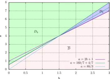
D2={(a, b) | 2b + 1 < a ≤ 8b/3},
D4={(a, b) | a > 8b/3 and a ≥ 16b/7 + 4/7},
D ={(a, b) | a ≤ 2b + 1 and a ≤ 16b/7 + 4/7}.
Proof: See Appendix.
Figure 1 shows these different domains and thus the benefit obtained by using either the 4-norm or the 2-norm.
It is easily checked in Figure 1 that the percentage of points (a, b) belonging to domain D4, which corresponds to the use
of the 4-norm, is much more greater than the percentage of points (a, b) belonging to domain D2, which corresponds to
the use of the 2-norm.
a b a = 2b + 1 a = 16b/7 + 4/7 a = 8b/3 0 1 2 3 4 5 6 7 8 0 0.5 1 1.5 2 2.5 3 D2 D4 D
Figure 1. Domains D2, D4and D for a∈ (0, 8] and b ∈ (0, 3].
In order to illustrate this figure with numerical values, we have for a = 2 and b = 1/4,
fn(2, 1/4) = 1 √ n and gn(2, 1/4) = 13 3n√n+ 48 n4
and Figure 1 shows, since (2, 1/4)∈ D4, that
P { ∥Y⌈2n ln(n)⌉∥∞≥ n1/41 } ≤ 13 3n√n+ 48 n4 ≤ 1 √ n.
For a = 7.5 and b = 3, we have
fn(7.5, 3) = 1 n1/2 and gn(7.5, 3) = 13 3n1/8 + 48 n4
and Figure 1 shows, since (7.5, 3)∈ D2, that
P { ∥Y⌈7.5n ln(n)⌉∥∞≥ n13 } ≤ 1 n1/2 ≤ 13 3n1/8 + 48 n4.
For a = 2 and b = 1, we have
fn(2, 1) = n and gn(2, 1) =
13n13/4
3 +
48
n
and Figure 1 shows, since (2, 1) ∈ D, that those values are useless to bound the quantity P{∥Y⌈7.5n ln(n)⌉∥∞≥ 1/n3}.
IX. EXPERIMENTALEVALUATION OF THECOUNTING
PROBLEMS
This section shows how tight our bounds are, by comparing the relation of Corollary 7 to the results obtained via extensive simulations in two cases, for the first κ = 0 and for the second
κ = n/2. We also compare these bounds to the ones obtained
by [7] in which the analysis is based on the 2-norm. The counting problem is equivalent to the proportion problem with
ε = 1/(2n), per example the counting problem with n = 1000
(see Figure 3) is like the proportion problem with ε = 0.0005, the advantage of this problem is that it could be compared with the results obtained in [7].
A simulation consists in the following steps: first, all the n nodes are initialized to m or −m (without loss of generality, we set m = 1). In the following, two scenario are discussed:
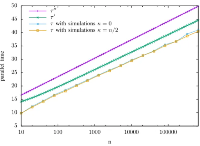
5 10 15 20 25 30 35 40 45 50 10 100 1000 10000 100000 parallel time n τ′′ τ′ τ with simulations κ = 0 τ with simulations κ = n/2
Figure 2. Parallel convergence time as a function of n when δ = 10−3and
N = 105 for n < 20000, N = 104for n > 20000. 18 20 22 24 26 28 30 32 34 36 38 1× 10⁻⁶ 1× 10⁻⁵ 0.0001 0.001 0.01 0.1 parallel time δ τ′′ τ′ τ with simulations κ = 0 τ with simulations κ = 500
Figure 3. Parallel convergence time as a function of δ when n = 103and
N = 106.
in the first one, 50% of the nodes are initialized to m and the other ones are initialized to −m (thus κ = 0), and in the second one, 75% of the nodes are initialized to m and the other ones are initialized to −m (thus κ = n/2). Then, at each step of the simulation, two nodes are randomly chosen to interact and update their state. The simulation stops when all the nodes output κ. We have run N independent simulations and have logged the N number of performed interactions
τ1≤ . . . ≤ τN. The convergence time is then τ⌈N(1−δ)⌉, with
δ ∈ (0, 1). Figures 2 and 3 depict the convergence parallel
time τ⌈N(1−δ)⌉/n (recall that the convergence parallel time is
equal to the convergence time divided by n) for both scenario, the bound τ′ obtained from Relation (7), and the bound τ′′ obtained from Theorem 4 of [7], i.e. τ′′= 4 ln 2+3 ln n−ln δ. Figure 2 clearly shows that the bound τ′given by Corollary 7 is very close to the parallel time obtained in the simulations, and greatly improves upon our previous results, i.e. τ′′. Figure 3 confirms the refinement of our theoretical evaluation. It shows that our present analysis is tighter than our previous one whatever the required precision of the computation.
X. CONCLUSION
In this paper we have presented a very precise analysis of the time required for each node to solve both the counting and
the proportion problems. Our work relies on the use of the 4-norm, and a comparison of bounds derived with both the 4-norm and the 2-norm shows the conditions under which it is beneficial to use the 4-norm or the 2-norm. We might sense that the use of the d-norm, for d > 4, would give more refined results but it would give rise to a much more intricate analysis.
REFERENCES
[1] Dan Alistarh, Rati Gelashvili, and Milan Vojnov´ıc. Fast and exact majority in population protocols. In Proceedings of the 34th annual
ACM symposium on Principles of distributed computing (PODC), pages
47–56, 2015.
[2] Dana Angluin, James Aspnes, and David Eisenstat. A simple population protocol for fast robust approximate majority. Distributed Computing, 20(4):279–304, 2008.
[3] James Aspnes and Eric Ruppert. An introduction to population protocols.
Bulletin of the European Association for Theoretical Computer Science, Distributed Computing Column, 93:98–117, 2007.
[4] Moez Draief and Milan Vojnovic. Convergence speed of binary interval consensus. SIAM Journal on Control and Optimization, 50(3):1087– 1097, 2012.
[5] M´ark Jelasity, Alberto Montresor, and Ozalp Babaoglu. Gossip-based aggregation in large dynamic networks. ACM Trans. Comput. Syst.,
23(3):219–252, 2005.
[6] George B. Mertzios, Sotiris E. Nikoletseas, Christoforos Raptopoulos, and Paul G. Spirakis. Determining majority in networks with local interactions and very small local memory. In Proceedings of the 41st
International Colloquium (ICALP), pages 871–882, 2014.
[7] Yves Mocquard, Emmanuelle Anceaume, James Aspnes, Yann Busnel, and Bruno Sericola. Counting with population protocols. In Proceedings
of the 14th IEEE International Symposium on Network Computing and Applications (NCA), pages 35–42, 2015.
[8] Yves Mocquard, Bruno Sericola, and Emmanuelle Anceaume. Optimal proportion computation with population protocols. In Proceedings of
the 15th IEEE International Symposium on Network Computing and Applications (NCA), pages 216–223, 2016.
[9] Etienne Perron, Dinkar Vasudevan, and Milan Vojnovic. Using three states for binary consensus on complete graphs. In Proceedings of the
APPENDIX
This appendix is dedicated to the proofs of Theorems 9, 10, 11, 12 and 13. Recall that we have defined Dn,1 and Dn,2 as
Dn,1= 4pn,A(1− pn,A) = ∥Y
0∥22
n and Dn,2= 16pn,A(1− pn,A)(3p
2
n,A− 3pn,A+ 1) = ∥Y
0∥44
n .
Recall also that, using (13), we have Dn,1≤ 1 and Dn,2≤ 4/3, for all n ≥ 1. Moreover, we will frequently use the inequality
for all x∈ [0, 1) and ν ≥ 0, (1 − x)ν≤ e−νx.
Theorem 9 For all a∈ (0, +∞) and n ≥ 3, we have E(∥Y⌈an ln(n)⌉∥22 ) ≤ n1−aD n,1≤ n1−a andE ( ∥Y⌈an ln(n)⌉∥22 ) ∼ n−→∞n 1−aD n,1.
Proof: When t =⌈an ln(n)⌉, we have from Realtions (8) and (10),
E(∥Y⌈an ln(n)⌉∥22 ) = ( 1− 1 n− 1 )⌈an ln(n)⌉ nDn,1≤ e−⌈an ln(n)⌉/(n−1)nDn,1 ≤ e−an ln(n)/(n−1)nD
n,1≤ e−a ln(n)nDn,1= n1−aDn,1≤ n1−a.
Following the same lines we also haveE(∥Yan ln(n)∥22
)
∼
n−→∞n
1−aD
n,1, which completes the proof.
In order to prove Theorems 10 and 11, we need the following lemma. We first introduce the notation γ = 1− 1
n− 1 and
we recall that α = 1− 2
n− 1 and β = 1−
7n− 6 4n(n− 1). Lemma 14: For all a∈ (0, +∞) and n ≥ 3, we have
α⌈an ln(n)⌉≤ n−2a and α⌈an ln(n)⌉ ∼
n−→∞n
−2a,
β⌈an ln(n)⌉≤ n−7a/4and β⌈an ln(n)⌉ ∼
n−→∞n
−7a/4,
γ⌈an ln(n)⌉≤ n−a and γ⌈an ln(n)⌉ ∼
n−→∞n
−a.
Proof: Setting t =⌈an ln(n)⌉, we easily obtain
β⌈an ln(n)⌉= ( 1− 7n− 6 4n(n− 1) )⌈an ln(n)⌉ ≤ e−(7n−6)⌈an ln(n)⌉/(4n(n−1))
≤ e−a(7n−6) ln(n)/(4(n−1))≤ e−7a ln(n)/4= n−7a/4.
The same lines lead to β⌈an ln(n)⌉ ∼
n−→∞n
−7a/4. In the same way we have
α⌈an ln(n)⌉= ( 1− 2 n− 1 )⌈an ln(n)⌉ ≤ ( 1− 2 n− 1 )an ln(n)
≤ e−2an ln(n)/(n−1)≤ e−2a ln(n)= n−2a
and also α⌈an ln(n)⌉ ∼
n−→∞n
−2a. The rest of the proof concerning γ is identical.
Theorem 10 For all a∈ (0, +∞) and n ≥ 3, we have E(∥Y⌈an ln(n)⌉∥42 ) ≤ D2 n,1n 2(1−a)+ 2(D n,2+ 3D2n,1)n
(4−7a)/4≤ n2(1−a)+ (26/3)n(4−7a)/4
and E(∥Y⌈an ln(n)⌉∥42 ) ∼ n−→∞ D2n,1n2(1−a) if a∈ (0, 4) 2(Dn,2+ 3D2n,1)n (4−7a)/4 if a∈ (4, +∞) (2Dn,2+ 7D2n,1)n−6 if a = 4.
Proof: From Corollary 5 and from Relation (11), we obtain
E(∥Yt∥42 ) = n n + 6 [ 2(Dn,2+ 3D2n,1)nβ t+ D2 n,1n 2αt− 2D n,2nαt ] .
Setting t =⌈an ln(n)⌉, using Lemma 14 and Relation (13) we get the inequalities and E(∥Y⌈an ln(n)⌉∥42 ) ∼ n−→∞2(Dn,2+ 3D 2 n,1)n (4−7a)/4+ D2 n,1n 2(1−a)− 2D n,2n1−2a.
For all a > 0, we have 1− 2a < 2(1 − a) and 1 − 2a < (4 − 7a)/4. Furthermore, 2(1 − a) ≥ (4 − 7a)/4 ⇐⇒ a ≤ 4. Thus E(∥Y⌈an ln(n)⌉∥42 ) ∼ n−→∞1{a≥4}2(Dn,2+ 3D 2 n,1)n (4−7a)/4+1 {a≤4}D2n,1n 2(1−a),
which completes the proof.
Theorem 11 For all a∈ (0, +∞) and n ≥ 3, we have E(∥Y⌈an ln(n)⌉∥44 ) ∼ n−→∞(Dn,2+ 3D 2 n,1)n (4−7a)/4 , E(∥Y⌈an ln(n)⌉∥44 ) ≤ 48n−1−2a+ (13/3)n(4−7a)/4.
Proof: From Corollary 5 and from Relation (12), we have
E(∥Yt∥44 ) = n n + 6 [ (Dn,2+ 3Dn,12 )nβ t+ 6D n,2αt− 3D2n,1nα t].
Setting t =⌈an ln(n)⌉ and using Lemma 14 we obtain E(∥Y⌈an ln(n)⌉∥44 ) ∼ n−→∞(Dn,2+ 3D 2 n,1)n (4−7a)/4 + 6Dn,2n−2a− 3D2n,1n−2a+1
Since for a > 0, (4− 7a)/4 > −2a + 1 > −2a, we have E(∥Y⌈an ln(n)⌉∥44 ) ∼ n−→∞(Dn,2+ 3D 2 n,1)n (4−7a)/4.
Now it is easy to check that 6Dn,2− 3D2n,1n≤ 48/n. We thus obtain
E(∥Y⌈an ln(n)⌉∥44
)
≤ 48n−1−2a+ (13/3)n(4−7a)/4.
which completes the proof.
We then have the following results for the distribution of∥Yt∥∞, with t =⌈an ln(n)⌉.
Theorem 12 For all a∈ (0, +∞), n ≥ 3 and ϵ > 0, we have P{∥Y⌈an ln(n)⌉∥∞≥ ε} ≤ n 1−a ε2 , P{∥Y⌈an ln(n)⌉∥∞≥ ε} ≤ n 2(1−a)+ (26/3)n(4−7a)/4 ε4 , P{∥Y⌈an ln(n)⌉∥∞≥ ε} ≤ 48n −1−2a+ (13/3)n(4−7a)/4 ε4 .
Proof: It suffices to use the inequality∥x∥∞≤ ∥x∥d and the Markov inequality. Indeed, using Theorem 9, we have
P{∥Y⌈an ln(n)⌉∥∞≥ ε} = P{∥Y⌈an ln(n)⌉∥∞2 ≥ ε2} ≤ P{∥Y⌈an ln(n)⌉∥22≥ ε 2} ≤ E ( ∥Y⌈an ln(n)⌉∥22 ) ε2 ≤ n1−a ε2 .
In the same way, using Theorem 10, we get
P{∥Y⌈an ln(n)⌉∥∞≥ ε} = P{∥Y⌈an ln(n)⌉∥∞4 ≥ ε4} ≤ P{∥Y⌈an ln(n)⌉∥42≥ ε 4} ≤ E ( ∥Y⌈an ln(n)⌉∥42 ) ε4 ≤ n2(1−a)+ (26/3)n(4−7a)/4 ε4 .
Finally, using Theorem 11, we obtain
P{∥Y⌈an ln(n)⌉∥∞≥ ε} = P{∥Y⌈an ln(n)⌉∥∞4 ≥ ε4} ≤ P{∥Y⌈an ln(n)⌉∥44≥ ε 4} ≤ E ( ∥Y⌈an ln(n)⌉∥44 ) ε4 ≤ 48n−1−2a+ (13/3)n(4−7a)/4 ε4 ,
which completes the proof.
Recall that the domains D2, D4 and D have been respectively defined by
D2={(a, b) | fn(a, b)≤ gn(a, b) and lim
D4={(a, b) | gn(a, b)≤ fn(a, b) and lim
n−→∞gn(a, b) = 0},
D ={(a, b) | lim
n−→∞fn(a, b)̸= 0 and limn−→∞gn(a, b)̸= 0},
where the bounds fn(a, b) and gn(a, b) are given by
fn(a, b) = n1−a+2b, gn(a, b) = 48n−1−2a+4b+
13 3 n
(4−7a+16b)/4.
Theorem 13 For all a∈ (0, +∞) and n ≥ 3, we have
D2={(a, b) | 2b + 1 < a ≤ 8b/3},
D4={(a, b) | a > 8b/3 and a ≥ 16b/7 + 4/7},
D ={(a, b) | a ≤ 2b + 1 and a ≤ 16b/7 + 4/7}.
Proof: Consider first domain D2. The condition limn−→∞fn(a, b) = 0 is equivalent to 1− a + 2b < 0, that is a > 2b + 1.
Moreover we have
fn(a, b)≤ gn(a, b)⇐⇒ 1 ≤ 48n2b−a−2+
13 3 n
2b−3a/4.
Thus, if a≤ 8b/3 then we have fn(a, b)≤ gn(a, b). Consider now domain D. The condition limn−→∞gn(a, b) = 0 is equivalent
to−1 − 2a + 4b < 0 and 1 − 7a/4 + 4b < 0, which is equivalent to a > 16b/7 + 4/7. We thus have
D ={(a, b) | a ≤ 2b + 1 and a ≤ 16b/7 + 4/7}.