The development and analysis of Scanned Pattern Interferometric Radar

(1)

by

Karen Marais

B.Eng., Electrical and Electronical Engineering University of Stellenbosch, South Africa, 1994

B.Sc., Mathematics

University of South Africa, 1997

SUBMITTED TO THE DEPARTMENT OF

AERONAUTICAL AND ASTRONAUTICAL ENGINEERING IN PARTIAL FULFILLMENT OF THE DEGREE OF

MASTER OF SCIENCE at the

MASSACHUSETTS INSTITUTE OF TECHNOLOGY

September 2001

Signature of

Certified by

A uthor ...

Department of Aeronautics and Astronautics August 24, 2001

Raymond J. Sedwick Research Scientist in the Departmej of Aeronautics and Astronautics Certified by Accepted by MASSACHIJSETS ISITUTE OF TECHNOLOGY

AUG 1 3 2002

LIBRARIES David W. Miller Director of the MJT Space Systerps Laboratory

Wallace E. Vander Velde Professor of Aeronautics and Astronautics Chair, Committee on Graduate Students

(2)

(3)

by

Karen Marais

Submitted to the Department of Aeronautics and Astronautics on August 24, 2001 in Partial Fulfillment of the Requirements for the Degree of Master of Science

at the Massachusetts Institute of Technology ABSTRACT

A method of performing space based GMTI using radar interferometric processing is pre-sented. The algorithm, referred to as Scanned Pattern Interferometric Radar (SPIR), uses the high angular variability of a sparse array Point Spread Function (PSF) to collect suffi-cient data from the signal return that the clutter and targets can be separated without an a priori assumption of the clutter statistics. By deconvolving the PSF from the received sig-nals the true ground scene is revealed. Performance of the algorithm is highly dependent on cluster design. Aperture placement in the cluster determines the (PSF). We show that minimum redundancy arrays are not appropriate for SPIR systems. An alternative design algorithm to select aperture placements that result in good SPIR performance is devel-oped. Numerical solution of SPIR systems by conventional linear algebra techniques is not feasible since the system conditioning is poor. The CLEAN algorithm, developed in the astronomical interferometry field, delivers promising results. Although clutter ampli-tude is random in nature, its position and doppler shift are geometrically related. An adapted version of CLEAN that uses this information shows improved target recovery. Prior target information can be used to further improve detection of both existing and new targets.

Thesis Supervisor: Dr. Raymond J. Sedwick

(4)

(5)

The opportunity to study at MIT has been the greatest of my life. A world that I did not know existed has been revealed to me. I would like to thank the following people: Ray-mond Sedwick, Tienie van Schoor, Rade Klaric, Elisabeth Lamassoure, John Enright, Joseph Saleh, and my parents, Sarel and Joan Marais.

This research was carried out under the supervision of Dr. Raymond Sedwick of the Space Systems Laboratory, MIT. I thank him for his guidance and support.

Tienie, you opened the door to MIT to me. Thank you for your unquestioning willingness to help.

Rade, you were unselfish enough to encourage me to embark on this voyage. My new world was your gift and I thank you for it.

Elisabeth, you became my best friend in your quiet and dignified way. I thank you for your support in all my endeavours, both academic and personal. You are wiser than you know and have taught me so much. I wish you all the best in your new life.

John, thank you for always being willing to help. Your insight has been invaluable in the creation of this thesis.

Joe, my debt to you is incalculable. If I have grown at all it is because of you. Mamma en Pappa, dankie vir alles. Wat ek ook al bereik kom van julle af.

(6)

(7)

. . . 5 . . . 7 11 15 . . . . 1 7 Chapter 1. Introduction . . . . 1.1 Historical Background . . . . 1.2 Spaceborne Radar . . . . 1.3 Multiple Aperture Systems . . . . 1.4 O utline . . . . Chapter 2. Radar Interferometry . . . . 2.1 Radar Concepts . . . . 2.1.1 Pulse-Doppler Radar . . . . 2.1.2 Radar Cross Section . . . . 2.1.3 The Radar Equation . . . . 2.1.4 Radar Clutter . . . . 2.2 Fourier Analysis . . . . 2.2.1 The Time Domain Fourier Transform . 2.2.2 The Spatial Fourier Transform . . . . . 2.2.3 Aperture Response . . . . 2.2.4 Brightness and Intensity . . . . 2.3 Fundamentals of Interferometry . . . . 2.3.1 Single Slit Aperture . . . . 2.3.2 Single Baseline Sparse Array . . . . . 2.3.3 Image Construction using Interferometry

. . . . 19 . . . . 2 0 . . . . 2 2 . . . . 2 3 . . . . 2 5 . . . 27 . . . 27 . . . 27 . . . 34 . . . 36 . . . 37 . . . 39 . . . 39 . . . 40 . . . 41 . . . 42 . . . 43 . . . 44 . . . 46 . . . 49 . . . 50 57 61 61 2.3.4 The Point Spread Function of an Interferometer . . . .

2.3.5 Interferometer System Design . . . . 2.4 Interferometric Techniques . . . . 2.4.1 Classical Displaced Phase Centre Antenna (DPCA) . . . .

7 Acknowledgments Table of Contents List of Figures . . . List of Tables . . . Nomenclature . . .

(8)

TABLE OF CONTENTS

2.4.2 Space-Time Adaptive Processing (STAP) . .

2.5 Summary . . . .

Chapter 3. Scanned Pattern Interferometric Radar . . 3.1 The SPIR Method . . . . 3.1.1 A Simplified Model of SPIR . . . . 3.1.2 Mathematical Derivation of SPIR . . . . 3.2 SPIR Implementation . . . . 3.2.1 Basic Processing Steps . . . . 3.2.2 Transmit/Receive Configurations . . . . 3.2.3 GMTI and the SPIR Method . . . . 3.2.4 SPIR Processing Load . . . .

3.2.5 Distributed SPIR Processing . . . .

3.3 Summary . . . .

Chapter 4. Point Spread Function Design . . . . 4.1 PSF Performance Measures . . . . 4.2 Construction of the PSF Matrix . . . . 4.3 PSF Design Parameters . . . . 4.3.1 PSF Spatial Period . . . . 4.4 Minimum Redundancy Arrays . . . . 4.4.1 Difference Bases . . . .

4.4.2 Application to Linear Antenna Arrays . . . .

4.4.3 Application of MRAs to SPIR . . . . 4.5 A Design Approach to Reduce Ambiguity . . . . . 4.5.1 Determining the Maximum Spatial Frequency 4.5.2 Optimally Irreducible Arrays . . . . 4.5.3 Aperture Placement . . . . 4.6 Evaluation of Arrays . . . . 4.6.1 Three Apertures . . . . 4.6.2 Four Apertures . . . . 4.6.3 Five Apertures . . . . 4.6.4 Discussion . . . . 4.7 Summary . . . . Chapter 5. SPIR System Modeling . . .

5.1 Solution of the SPIR System . . . .

62 63 65 65 66 68 72 73 74 75 79 82 88 . . . . 89 . . . . 89 . . . . 90 . . . . 92 . . . . 92 . . . . 95 . . . . 96 . . . . 99 . . . 102 . . . 103 Number . . . 103 . . . 104 . . . 106 . . . 106 . . . 107 . . . 107 . . . 110 . . . 112 . . . 112 . . . 113 . . . 113 8

(9)

5.1.2 Deconvolution and System Conditioning . .

5.2 Deconvolution using CLEAN . . . . 5.2.1 The CLEAN Algorithm . . . . 5.2.2 Application of CLEAN to SPIR . . . . 5.2.3 Improving SPIR Performance Using CLEAN

115 117 117 120 127 5.3 Summary . . . 133

Chapter 6. Summary and Future Work . . . 135

6.1 Summary . . . 135

6.2 Future W ork . . . 137

References . . . 139

Appendix A. Example Linear Clusters . ... A.1 Six Apertures ... A. 1.1 Unrestricted ... A.1.2 Restricted ... A.2 Seven Apertures . . . . A.2.1 Unrestricted . . . . A.2.2 Restricted . . . . A.3 Eight Apertures . . . . A.3.1 Unrestricted . . . . A.3.2 Restricted . . . . A.4 Nine Apertures . . . . A.4.1 Unrestricted . . . . A.4.2 Restricted . . . . A.5 Ten Apertures . . . . A.5.1 Unrestricted . . . . A.5.2 Restricted . . . . A.6 Eleven Apertures . . . . A.6.1 Unrestricted . . . . A.6.2 Restricted . . . . A.7 Twelve Apertures . . . . A.7.1 Unrestricted . . . . A.7.2 Restricted . . . . . . . 141 . . . 142 . . . 142 . . . 143 . . . 144 . . . 144 . . . 146 . . . 148 . . . 148 . . . 150 . . . 152 . . . 152 . . . 152 . . . 154 . . . 154 . . . 154 . . . 156 . . . 156 . . . 157 . . . 157 . . . 157 . . . 158

(10)

10 TABLE OF CONTENTS

Appendix B. SIngular Value Decomposition ... 159

B.1 The Singular Value Decomposition . . . 159

B.2 Solution of Non-Full Rank Systems using SVD . . . 162

Appendix C. Matlab Code . . . 165

C.1 M aster File . . . 165

C.2 Implementation of CLEAN . . . 171

(11)

Figure 2.1 Figure 2.2 Figure 2.3 Figure 2.4 Figure 2.5 Figure 2.6 Figure 2.7 Figure 2.8 Figure 2.9 Figure 2.10 Figure 2.11 Figure 2.12 Figure 2.13 Figure 2.14 Figure 2.15 Figure 3.1 Figure 3.2 Figure 3.3 Figure 3.4 Figure 3.5 Figure 3.6 Figure 3.7 Figure 3.8 Figure 3.9 Figure 3.10 Figure 3.11 Figure 4.1 Range Ambiguity . . . . Doppler Ambiguity . . . . Range Gating . . . . The Corner-Turn FFT . . . . Ground Clutter Observed by a Forward-Lc Platform . . . . Single Slit Amplitude Distribution . . . Single Slit Aperture Point Spread Function Two Pinhole Amplitude Distribution Two Pinhole Point Spread Function .

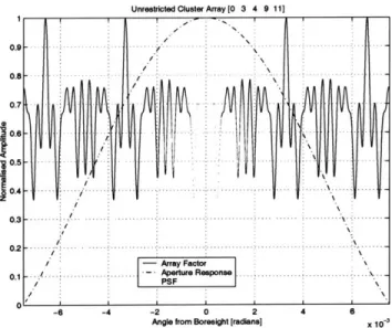
Calculation of the PSF using the Fourier T

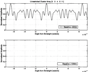
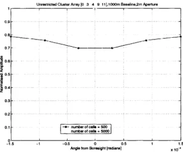
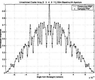
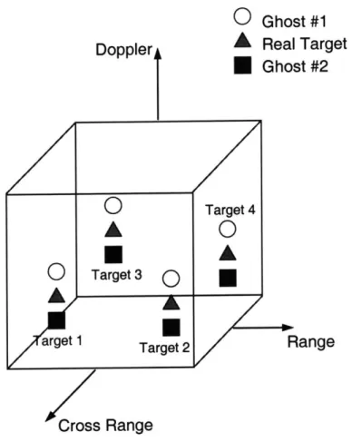
31 33 34 oking Ai ransform Construction of the PSF . . . . Effect of Array Baseline on the PSF . . . . PSF Sampled at Two Different Rates . . . . Sampling the PSF . . . . Side-looking Linear Cluster . . . . The SPIR Concept . . . . Relative Signal Delay . . . . Basic SPIR Implementation . . . . Single Transmitting Aperture . . . . All Apertures Transmit and Receive . . . . SPIR Data Cube . . . .

Footprint with a Single Range Ambiguity . . . .

Using PRF Jitter to Eliminate Doppler Ambiguities

Processing Load Distribution by Range Gate . . .

Broadcast Communication . . . . Four and Eight Element Hypercubes . . . . Construction of a PSF Matrix . . . . . . . . 35 r- or Spaceborne Radar . . . . . 38 . . . . . 44 . . . . . 46 . . . . . 47 . . . . . 48 . . . . 51 . . . . . 53 . . . . . 54 . . . . . 55 . . . . . 57 . . . . . 58 . . . . . 67 . . . . . 69 . . . . . 73 . . . . . 74 . . . . . 75 . . . . . 76 . . . . . 77 . . . . 78 . . . . . 85 . . . . . 86 . . . . . 87 . . . . . 91

(12)

12 LIST OF FIGURES

Figure 4.2 Construction of a Ambiguous PSF Matrix . . . . Figure 4.3 Array Spread . . . . Figure 4.4 Array Redundancy . . . . Figure 4.5 Three Element Optimally Irreducible Array . . . Figure 4.6 Four Element Optimally Irreducible Array . . . . Figure 4.7 Four Element Optimally Irreducible Array . . . . Figure 4.8 Four Element Optimally Irreducible Array . . . . Figure 4.9 Four Element Optimally Irreducible Array . . . . Figure 4.11 Five Element Optimally Irreducible Array . . . . Figure 4.10 Four Element Optimally Irreducible Array . . . . Figure 4.13 Five Element Optimally Irreducible Array . . . . Figure 4.12 Five Element Optimally Irreducible Array . . . . Figure 5.1 Singular Values for G and |G| . . . . Figure 5.2 The CLEAN Algorithm . . . . Figure 5.3 CLEAN Recovery of Two Closely Spaced Targets

Apertures) . . . . Figure 5.4 CLEAN Recovery of Two Closely Spaced Targets

(Cells 40 and 42) (Cells 40 and 45) (3 (3 121 Apertures) . . . 122

Figure 5.5 CLEAN Recovery of Two Targets at the Edges of the Footprint (3 Aper-tures) . . . 123

Figure 5.6 CLEAN Recovery of Two Targets at the Edges of the Footprint with Smaller Threshold (3 Apertures) . . . 123

Figure 5.7 CLEAN Recovery with a Target at the Footprint Centre (3 Apertures) 124 Figure 5.8 CLEAN Recovery with Centre Targets (3 Apertures) . . . 125

Figure 5.9 CLEAN Recovery with Targets and Clutter (3 Apertures) . . . 125

Figure 5.10 CLEAN Recovery with Targets and Clutter (8 Apertures) . . . 126

Figure 5.11 Clutter Reduction using CLEAN . . . 129

Figure 5.12 Improved CLEAN Recovery with Clutter (12 Apertures) . . . 129

Figure 5.13 Improved CLEAN Recovery with Large Clutter (12 Apertures) . . . . 130

Figure 5.14 Improved CLEAN Recovery with Targets and Randomly Varying Large Clutter (12 Apertures) . . . 131

Figure 5.15 Improved CLEAN Recovery with Targets and Randomly Varying Large Clutter Spread Across Multiple Cells (12 Apertures) . . . 131

. . . . 92 . . . 100 . . . 102 . . . 107 . . . 108 . . . 108 . . . 109 . . . 109 . . . 110 . . . 110 . . . 111 . . . 111 . . . 117 . . . 119

(13)

Figure A.1 Figure A.2 Figure A.3 Figure A.4 Figure A.5 Figure A.6 Figure A.7 Figure A.8 Figure A.9 Figure A.10 Figure A.11 Figure A.12 Figure A.13 Figure A.14 Figure A.15 Figure A.16 Figure A.17 Figure A.18 Figure A.19 Figure A.20 Figure A.21 Figure A.22 Figure A.23 Figure A.24 Figure A.25 Figure A.26 Figure A.27 Figure A.28 Figure A.29 Figure A.30

Six Element Optimally Irreducible Array (Unrestricted) . . . 142

Six Element Optimally Irreducible Array (Restricted) . . . 143

Seven Element Optimally Irreducible Array (Unrestricted) . . . 144

Seven Element Optimally Irreducible Array (Unrestricted) . . . 145

Seven Element Optimally Irreducible Array (Restricted) . . . 146

Seven Element Optimally Irreducible Array (Restricted) . . . 147

Eight Element Optimally Irreducible Array (Unrestricted) . . . 148

Eight Element Optimally Irreducible Array (Unrestricted) . . . 149

Eight Element Optimally Irreducible Array (Restricted) . . . 150

Eight Element Optimally Irreducible Array (Restricted) . . . 151

Nine Element Optimally Irreducible Array (Unrestricted) . . . 152

Nine Element Optimally Irreducible Array (Restricted) . . . 152

Nine Element Optimally Irreducible Array (Restricted) . . . 153

Ten Element Optimally Irreducible Array (Restricted) . . . 154

Ten Element Optimally Irreducible Array (Restricted) . . . 155

Eleven Element Optimally Irreducible Array (Unrestricted) . . . 156

Eleven Element Optimally Irreducible Array (Restricted) . . . 157

Twelve Element Optimally Irreducible Array (Unrestricted) . . . 157

(14)

14 LIST OF FIGURES

Figure B. 1 SVD of a 2x2 Matrix (adapted from [Trefethen, 1997]) . . . 160 Figure B.2 Singular Value Removal . . . 163

(15)

TABLE 3.1 TABLE 4.1 TABLE 4.2 TABLE 4.3 TABLE 5.1

Representative System for Processing Load Calculation . . . . Unrestricted Difference Bases, up to 11 Apertures . . . . Restricted Difference Bases, up to 11 Apertures . . . . System Parameters . . . . System Parameters . . . . 79 97 98 106 120

(16)

(17)

AMTI Airborne moving target indication

A Area [m2]

c Speed of light [m/s]

CFAR Constant False Alarm Rate

CW Continuous Wave

d Diameter [m]

DFT Discrete Fourier Transform

DPCA Displaced Phase Centre Antenna

E Electric field intensity [V]

f

Frequency [Hz]

fc

Carrier frequency [Hz]

GMTI Ground moving target indication g Gravitational acceleration [m/s2]

h Height [m]

i Current [A]

Carrier wavelength [m]

1 Length [m]

MTI Moving target indication

PRF Pulse Repetition Frequency [Hz] PRI Pulse Repetition Interval [s]

r Radius [m]

Rearth Radius of the earth

SPIR Scanned Pattern Interferometric Radar

sr Steradian

STAP Space Time Adaptive Processing

T Pulse width [s]

(18)

(19)

INTRODUCTION

The recent demise of MIT's Building 20 brought to mind a remarkable era of discovery, much of which took place here at the Massachusetts Institute of Technology. Designed in an afternoon, and erected in just six months in 1943, Building 20 was the heart of the Radiation Laboratory, affectionately known as RadLab. Here, during the frenzied war years, a remarkable collaboration between the British and the Americans, the military and civilians, resulted in discoveries that would eventually impact all aspects of modem life. Radar, an acronym for RAdio Detection And Ranging, is based on the deceptively simple concept of locating objects using transmitted and reflected high-frequency radio waves. Waiting in the wings for technology to advance, it was seized on by eager governments at its first appearance. The ensuing fifty-odd years have seen an explosion in radar applica-tions, both in the civilian and military worlds.

Ground Moving Target Indication (GMTI) using separated spacecraft interferometry at radio wavelengths promises to be a powerful new all-weather surveillance tool. GMTI radar is frequently implemented on both ground-based and airborne systems, but space-borne systems are less common. This thesis develops and analyses a novel processing algorithm by which radar data from separated spacecraft can be combined to yield high resolution radar maps.

(20)

20 INTRODUCTION

1.1 Historical Background

In 1873, James Clark Maxwell published his landmark work unifying the equations gov-erning electromagnetic waves, Treatise on Electricity and Magnetism. Nearly fifteen years later, Heinrich Hertz conducted a classic series of experiments in which he generated and detected radio waves. He showed that the waves travelled at the speed of light and could be reflected, refracted, diffracted and polarized like visible light, as Maxwell had pre-dicted. The discovery inspired scientists across the world. When Guglielmo Marconi suc-cessfully sent radio signals across the Atlantic in 1901 the modern communications industry was born.

Credit for the invention of radar cannot be given to a single person. Hertz's experiments had showed that electromagnetic waves could be bounced off objects. Both Nikolai Tesla and Marconi realised that objects could be detected by bouncing radio signals off them. By patenting a radio echo device for locating objects at sea, a German engineer named Christian Hulsmeyer proclaimed himself the inventor of radar in 1904.

The idea was not practicable at the time however. The technology to generate high fre-quency signals, with wavelengths shorter than 50 m did not exist. Low frefre-quency signals could not maintain sufficient focus over long distances to be detectable. It took years of technological advancement before radar could come into its own.

Rightly or wrongly known as the father of radar, Sir Robert Watson-Watt and his junior scientific officer Arnold F. "Skip" Wilkins proposed the concept of using radio waves to detect aircraft to the British government in 1935. The Air Ministry had offered a E1000 reward for anyone who could design a "death" ray that could kill a sheep at a hundred yards. In his capacity as superintendent of the Radio Department of the National Physics Laboratory, Watson-Watt quickly determined that the idea was not feasible at the time. He did come up with an alternative proposal however:

"Meanwhile attention is being turned to the still difficult but less unprom-ising problem of radio-detection as opposed to radio-destruction, and

(21)

numerical considerations of the method of detection by radar waves will be submitted when required."

Nervous about the growing threat from Hitler's Germany, and with no means of protecting Britain against an air attack, the British government pounced on Watson-Watt's idea, requesting the promised facts and figures. Watson-Watt turned to Wilkins to perform the detailed calculations. The results were so inspiring that an excited Watson-Watt immedi-ately drafted a memo that would become a landmark in the history of radar, "Detection of Aircraft by Radio Methods" on February 12, 1935.

Following Watson-Watt's proposals, the Chain Home network was created along Britain's east and south coasts. It was a system of antennas that could detect aircraft up to 150 miles away. During the London Blitz the system provided early warning of incoming bombing raids, saving countless lives.

British scientists aggressively experimented with shorter wavelengths, narrower beams, more compact equipment, and greater power generation to improve their radar capability. In 1940 Watson-Watt, together with John Randall and Henry Boot, invented the cavity magnetron. The magnetron was a compact source of high frequency radio waves that could be used over distances on the order of tens of kilometres to detect small, airborne targets.

In August 1940, the British government dispatched the top-secret Tizard Mission to the United States to exchange information on radar. In a pivotal meeting the British revealed their resonant cavity magnetron. The magnetron, an efficient, high-power (10-kilowatt) pulsed oscillator that operated at 10 centimetre wavelengths, was the seed for the British-American collaboration, centered at the newly created MIT Radiation Laboratory.

The laboratory's first three projects focussed on protection of Britain. Project I created a 10 cm airborne intercept radar that would enable bombers to detect enemy aircraft at night. Project II developed the highly successful SCR-584 gun-laying radar, which is cred-ited with leading to the safe destruction of 85% of the V- 1 buzz bombs that were dropped

(22)

22 INTRODUCTION

on London. Project III developed a long range navigation system for ships and aircraft, known as LORAN (LOng RAnge Navigation), which is still in use today.

Building 20 began as a collaboration between Britain and the United States to make microwave radars. It rapidly developed into a centralised laboratory, which laid much of the theoretical radar groundwork while simultaneously creating working systems for use in the Allied war effort. In the years from 1940 to 1945 RadLab designed over one hun-dred different radar systems, which comprised close to half of the radar systems deployed in World War II, and had a monetary value of $1.5 billion.

Radar has not failed to deliver on its promise. Since the heady days of RadLab radar has been adapted for many purposes. These include high-resolution mapping of ocean levels, freeway speed enforcement, air-traffic control and many military applications.

Spaceborne radar was initially used as an aid for space rendezvous, on the Gemini space-craft. It was not long before radar antennas were turned towards Earth and in present day the primary application of space-based radar has become observation. Spaceborne radar permits high resolution and high fidelity observation of the entire surface of Earth regard-less of weather conditions. It is not surprising that a wide range of applications have been found in both the military and civilian worlds. Applications include altimetry, ocean level observation, weather observation, terrain mapping, and navigation.

The interested reader is invited to consult Robert Buderi's fascinating account of the development of radar at the Radiation Laboratory, The Invention that Changed the World [Buderi, 1996].

1.2 Spaceborne Radar

GMTI is typically used to locate large vehicles such as tanks and trucks in military appli-cations. Current systems, such as JSTARS (Joint Surveillance Target Attack Radar Sys-tem, a US Air Force Research Project), use airborne platforms to provide temporary

(23)

coverage in regions of interest. These systems provide good performance but require large support infrastructures and significant deployment time and require pilots to fly in active theatres. Spaceborne radar can offer nearly continuous global coverage without apprecia-ble operator risk.

As discussed by Shaw [Shaw, 1998], there are three fundamental design considerations for spaceborne radar. First, the radar must have sufficient power-aperture product to detect targets at the required search rate. Second, the angular and range resolution must be high enough to locate the target with the required degree of accuracy. Third, the radar must reject clutter and noise sufficiently to provide the specified probability of detection and false alarm rate. Thus, development of an effective spaceborne radar system presents many challenges.

In this thesis we discuss the design and implementation of a spaceborne GMTI interfero-metric radar system. We address high-level system design aspects and describe a novel processing algorithm by which images can be constructed.

1.3 Multiple Aperture Systems

Single aperture systems are a compromise between high resolution and broad coverage. Broad coverage, or large field of view, requires a wide beamwidth, while high resolution requires a narrow beamwidth.

Unwanted return from the ground, known as clutter, presents an additional challenge. Clutter suppression is computationally intensive and requires prior knowledge of the tar-get as well as an appropriate clutter model. Performance is therefore limited by the quality of prior target information and the accuracy of the clutter model.

In contrast, multiple aperture systems can provide coverage corresponding to the diameter of a single aperture and resolution proportional to the maximum separation between

(24)

24 INTRODUCTION

Space-Time Adaptive Processing (STAP) has been proposed for use in multiple aperture systems [Ward, 1994]. STAP takes advantage of the high resolution properties of the inter-ferometer, but does not use all the information available in the return signals. Like single aperture methods, STAP is limited by the accuracy of the clutter model. Good prior esti-mates of the position and velocity of any targets are required. Careful maintenance of aperture positions in the cluster is necessary to achieve an adequate level of clutter sup-pression.

TECHSAT21 is a technology demonstrator program with an experimental multiple aper-ture radar payload. It consists of a cluster of microsatellites (less than 100 kg) that orbit in close proximity (on the order of hundreds of metres). Each microsatellite is capable of coherently detecting not only return signals resulting from its own transmission, but also return signals resulting from the transmissions of other satellites in the cluster.

Scanned Pattern Interferometric Radar (SPIR) combines the individual aperture signals in a way that allows ground clutter to be characterized completely and removed. This method depends not on the statistics of the clutter, but solely on the clutter position and doppler shift. While the clutter amplitude and phase are random in nature, the doppler shift is entirely predictable due to the known angular location of the clutter footprint. The algo-rithm relies on "deconvolving" the gain pattern of the synthesized aperture from the received signals to reveal the true ground scene.

In conventional interferometry, deconvolution is usually performed entirely in the spatial domain, and removes the artefacts that appear in the image as a result of incomplete (u, v) plane filling. SPIR processing uses the distinctive features of the interferometer response,

and their effect on both spatial and frequency information, to separate ground clutter return from target return. The statistical nature of the clutter is irrelevant and the

(25)

1.4 Outline

This thesis develops and analyses the Scanned Pattern Interferometric Radar method, beginning with the initial intuitive concept and concluding with a simulated implementa-tion.

A description of the process begins with some fundamentals of radar and interferometry in Chapter 2. Chapter 3 describes SPIR and gives a mathematical derivation. Optimum placement of apertures within the cluster is discussed in Chapter 4. Solution of SPIR sys-tems is not trivial, Chapter 5 examines this problem. Chapter 6 gives conclusions and rec-ommends future work.

(26)

(27)

RADAR INTERFEROMETRY

Scanned Pattern Interferometric Radar (SPIR) borrows techniques from the field of inter-ferometry to create high-resolution radar systems. Understanding radar interinter-ferometry therefore requires an appreciation for both radar and interferometric imaging theory. To that end, this chapter discusses background material. We begin with a short discussion of some radar concepts that are necessary to understand Scanned Pattern Interferometric Radar (SPIR). Fourier analysis is a powerful tool of which we make much extensive use in SPIR. A summary of useful Fourier techniques is provided. Finally, the last two sections discuss interferometry techniques, with specific reference to radar applications.

2.1 Radar Concepts

In this section we introduce some concepts that will aid in the understanding of SPIR. Readers unfamiliar with radar are referred to [Stimson, 1998] for an excellent introduc-tion.

2.1.1 Pulse-Doppler Radar

Radar has many applications, from ground mapping to altimetry to moving target indica-tion. Ground mapping radar maps stationary objects and may have very high resolution on the order of millimetres. Altimetry measures the altitude of air- or spaceborne objects. Moving Target Indication (MTI) radar searches for targets that may be on the ground or air

(28)

28 RADAR INTERFEROMETRY

(space) borne. MTI radar has an additional source of information on targets, namely their closing velocity. Most MTI radars are of a specific type referred to as pulse-doppler radar. There are two general types of radar transmitter, Continuous Wave (CW) and pulsed. CW radar continuously transmits and receives. The main problem with air- and spaceborne CW radars is electrical noise, or interference. The limited available space makes it diffi-cult to physically isolate the transmitter from the receiver. As a result noise arising from generation of the high energy transmitted signal corrupts the received echoes, preventing accurate radar mapping. Pulsed radar eliminates this problem by transmitting short pulses and listening for the reflected echoes in the intervals between transmissions. Pulsed radars that sense doppler frequency are called pulse-doppler radars, those which only sense range are simply called pulse radars.

The Pulsed Waveform

The pulsed waveform has four basic characteristics: carrier frequency,

f,

[Hz], pulse width, t [s], interpulse modulation, and pulse repetition frequency, PRF [Hz].

The carrier frequency is usually chosen based on physical size limitations, available trans-mitted power, and atmospheric attenuation characteristics. In the case of air- and space-borne systems the choice of carrier frequency is dominated by the size limitations inherent on a satellite. As frequency is increased, RF analog processing hardware dimensions decrease and the antenna diameter required to provide a given beamwidth decreases. The maximum beamwidth should be comparable with the expected region of interest; this ensures that transmission energy is not "wasted" outside the region of interest. The X-band (10GHz) is popular for space-based radar applications since radar hardware dimen-sions are compatible with satellite size limitations while atmospheric attenuation is still reasonably low.

The pulse width determines the highest possible resolution of the radar in the range direc-tion. Range resolution is defined as the minimum range between two objects at which they can be resolved.

(29)

The extent of a pulse in space is

L = cT (2.1)

Objects that are more closely spaced than L/2 cannot be resolved. Increasing the resolu-tion therefore requires decreasing the pulse length. Decreasing the pulse length decreases the energy contained in the pulse. Since the peak power that a radar can transmit is limited by size and mass constraints, very narrow pulses will not contain enough energy to allow target detection.

Pulse width therefore seems to place a limit on the range resolution. However, if the effec-tive pulse width is decreased while the actual pulse is kept sufficiently wide to ensure tar-get detection, good range resolution can be obtained. This can be achieved by encoding the transmitted pulse in frequency and/or phase so that the received pulse can be com-pressed before target detection is performed. Two popular techniques are chirp compres-sion, where the frequency of the carrier is linearly increased over the length of the pulse, and binary phase modulation, where successive chips of the pulse have their phase changed by 0* or 1800.

The pulse repetition frequency (PRF) is the rate at which the pulses are transmitted. The inverse of the PRF is the pulse repetition interval (PRI). The choice of PRF determines to what extent the ranges and doppler frequencies sensed by the radar will be ambiguous, as discussed in the next two sections.

The probability of detection of a target is directly related to the amount of signal energy that illuminates it. In addition to using pulse compression to increases the individual pulse energy, the received echoes from several successive pulses are usually summed. This pro-cess is referred to as pulse integration. The number of pulses integrated is selected to be sufficiently low that there is no appreciable change in the targets' positions and velocities during the integration time.

(30)

Pulse Integration

There are two ways of integrating the signal returns from multiple pulses: coherent and non-coherent integration.

Coherent integration is performed on the signal before it has been stripped of its carrier, hence phase is preserved. Non-coherent integration is performed on the modulating signal

(envelope), which does not carry phase information.

If n pulse are coherently integrated, in the ideal case the resulting signal to noise power ratio would be n times that of a single pulse. Non-coherent integration always has a gain

less than n, due to information loss in the envelope detection process.

However, since non-coherent integration is easier to implement, it is more popular. Thresholding

The process of deciding whether a given signal return corresponds to a target or noise is called thresholding. In essence, signals that are greater than a certain level, or threshold, are declared to be targets, whereas smaller signals are assumed to be noise. The selection of the threshold is therefore crucial. If the threshold is too high, small targets may be missed. If the threshold is too low, noise spikes may be mistaken for targets.

The threshold directly affects the probability of detection (Pd) as well as the probability of false alarm (PFA). An ideal system would have a high Pd and a low PFA. Unfortunately these requirements conflict with each other. Current systems settle for a constant false alarm rate (CFAR), which depends on the required Pd. CFAR processing is complex and the literature abounds with references. [Skolnik, 1980] is a good starting point.

Measuring Range

Range measurement with pulsed radar is simple. The range to the target can be determined by measuring the time interval t between transmission of the pulse and its reception

(31)

range = Ct (2.2)

2 where c is the speed of light.

This method of ranging works as long as the round trip time for the pulse is less than the interpulse period. If the radar detects a target whose round-trip time is larger than the interpulse period, the echoed pulse will appear to come from a subsequent pulse, as shown in Figure 2.1. The resulting calculated range is ambiguous since it is impossible to deter-mine which of the transmitted pulses it corresponds to.

received pulse transmitted pulses

PRI time

True Range Apparent Range

Figure 2.1 Range Ambiguity

The maximum range from which return may be received without the observed range being ambiguous is called the unambiguous range R,

R = C (2.3)

2.PRF

At high PRF's measured ranges are likely to be ambiguous, as many targets may fall out-side RU. Range ambiguities can be avoided by setting Ru greater than the maximum expected target range. However, at low PRF's doppler ambiguities appear, as discussed in the next section.

(32)

32 RADAR INTERFEROMETRY

The Doppler Effect

The doppler effect is the shift in frequency experienced by any type of wave that is radi-ated, reflected, or received by a moving object. It is commonly observed when standing on the side of a road listening to a car passing at high speed. The pitch of the sound is higher when the car is approaching than when it is receding. When objects approach one another the doppler shift is positive, and when they are receding from each other the doppler shift is negative.

In radar the doppler effect is used to determine the relative velocity between the radar antenna and the object(s) it is tracking. The doppler frequency shift is related to the clos-ing velocity as follows

Vlo sing

fdoppler = 2 v (2.4)

where X is the wavelength of the carrier. Given the radar platform's velocity, the target's velocity along the line of sight (LOS) to the radar can be determined. In spaceborne radar three relative motions contribute to the observed doppler shift: the Earth's rotation, the sat-ellites' orbit and the object's motion.

Doppler ambiguities occur when the PRF is low. Since the radar pulses are the observed scene at the PRF, the frequency spectrum of the radar return is repeated at the PRF. Targets with doppler frequencies greater than the PRF will be undersampled and appear to have lower doppler frequencies, as shown in Figure 2.2.

At low PRFs measured doppler frequencies are likely to be ambiguous, since target dop-pler shifts may be greater than the PRF. Dopdop-pler ambiguities can be avoided by setting the PRF higher than the expected doppler shift bandwidth. However, as we have seen in the previous section, this introduces range ambiguities.

(33)

Doppler Bandwidth

-2PR -PRO

l0

IPRF4 12PRF frequency

True Doppler

| |

Apparent Doppler ' J

Figure 2.2 Doppler Ambiguity

Range and doppler ambiguities can be alleviated by varying the pulse repetition frequency (PRF), this is known as PRF switching or jittering. Refer to [Stimson, 1998] for a detailed description of this technique.

Range Gating and Doppler Filtering

Digitally sampling the received radar signal allows the use of sophisticated processing algorithms. Therefore, in modem radars most processing is performed on a digitally sam-pled version of the signal. Although analog versions of some processes described here were used in the past, this discussion is restricted to the digital processes.

The first steps in processing are range gating and doppler filtering.

Range gating is the process of assigning (ambiguous) ranges to the received signal sam-ples. Ideally, each signal sample corresponds to a particular ambiguous range, or range gate. However, individual signal samples are likely to be corrupted by noise. Therefore, a range gate will usually straddle several samples and average their contributions in some manner. By overlapping the range gates, as shown in Figure 2.3, range resolution can be maintained.

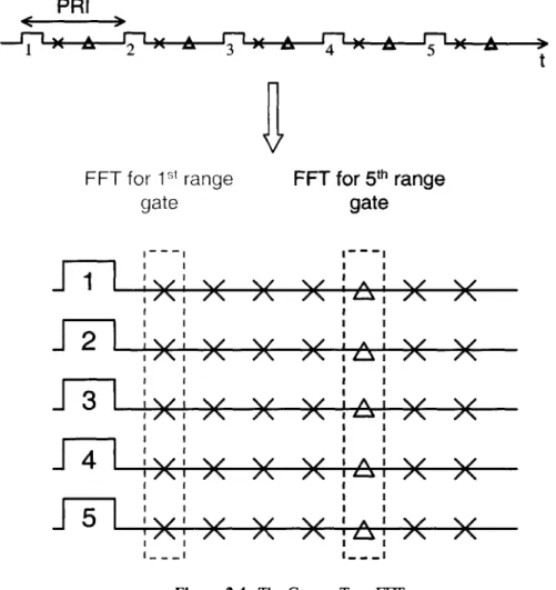
The next step is to determine the doppler frequency content of each range gate. The pro-cess is referred to as the corner-turn FFT (fast Fourier transform) and is illustrated in

(34)

1st gate 2nd gate

lit

I

1 0

Range resolution

Figure 2.3 Range Gating

Figure 2.4. The FFT is a computationally efficient implementation of the Discrete Fourier Transform (DFT). Returns from successive pulses are placed below each other and an FFT is taken for each range gate. The sampling rate for the FFT is therefore equal to the PRF.

2.1.2 Radar Cross Section

The radar cross section (RCS) of an object is an indication of the amount of reflected energy the radar will receive from that object. It is commonly indicated by a and is a function of the geometric cross section, reflectivity and directivity of the object

Geometric

a Cross x (Reflectivity) x (Directivity) (2.5)

Section

The geometric cross section, Aobject ' is the area of the object as seen from the radar. This

area determines how much signal power the object will intercept

intercepted transmitted xobject (2.6)

The reflectivity indicates how much of the intercepted signal power the object reflects, or scatters

Reflectivity = scatter (2.7)

(35)

PRI t FFT for 1st range gate

174

5

-- I FFT

for

5 th

range

gate

I I \J NY ..A.I N

Figure 2.4 The Corner-Turn FFT

The directivity is the ratio of the power scattered back in the radar's direction to the power that would have been scattered isotropically

Directivity = P backscatter

Disotropic (2.8)

Normally Pbackscatter and Pisotropic are expressed as power per unit solid angle (dian). Pisotropic is then equal to the total scattered power divided by the number of stera-dians in a sphere

isotropic scatter (2.9)

Isotro4n

711

(36)

The directivity can therefore be expressed as

Directivity = backscatter (2.10)

(1/4n)Pscatter

In the case of reflection from the ground, the ground is characterised in terms of the incre-mental backscattering coefficient, ao . It is the radar cross section of a unit area of ground.

2.1.3 The Radar Equation

The radar equation predicts the detection range of a radar based on the characteristics of the radar, target and environment. One form of the equation is

p - Paverage GaAetint

received = 2 4 (

(4nt)RL

where

Preceived = Received power

Paverage = Average transmitted power

G = Antenna gain

a = Target RCS (2.12)

Ae = Effective antenna area

tint = Integration time

R = Range

L = Loss factor

The received power decreases as range to the fourth. This means that at long ranges the received power will be significantly lower than the transmitted power. The probability that a target will be detected is directly related to the received power. For a given target and range the probability of detection can be improved by increasing the transmitted power, integration time or effective antenna area, or by decreasing the system losses L.

(37)

The integration time is the time that the radar illuminates the footprint. As the integration time is increased, the signal to noise ratio of the integrated signal is increased. Increased dwell time also results in higher frequency resolution, which aids in clutter rejection. However, the integration time must be sufficiently short that the relative velocity between the cluster and the footprint does not change appreciably, as this decreases the accuracy of the doppler measurements. The integration time directly affects probability of detection, false alarm rate and doppler frequency measurement accuracy and should be carefully chosen to obtain the desired system performance.

The design of spaceborne Earth-observing radars presents additional challenges since the available transmission power is limited and the received signal is severely attenuated by the large range. Excellent clutter and noise rejection characteristics are essential for suc-cessful systems.

2.1.4 Radar Clutter

Any unwanted radar return is referred to as clutter. In a ground-mapping radar, return from the ground is desired, and is used to construct the ground map. However, in the case of moving target indication (MTI) radar, return from the ground obscures, or clutters, the desired target return.

Ground clutter is commonly classified into three categories: main lobe return, side lobe return, and altitude return. Main lobe and side lobe return is collected by the radar antenna's main and side lobes respectively. Altitude return is side lobe return received from directly beneath the antenna and appears at a range corresponding to the altitude of the antenna above the ground. Figure 2.5 shows a typical ground clutter profile seen by an airborne or spaceborne radar, as a function of doppler frequency. Main lobe clutter has a higher average amplitude than side lobe clutter, since the main lobe antenna gain is higher. Altitude return has a high average amplitude since it experiences the least scattering.The doppler shift experienced by clutter from a specific patch on the ground can be predicted based on the geometric relationship between the ground patch and the antenna.

(38)

2

vradarcoso (2.13)

fdoppler

x

'

where 0 is the angle between the antenna velocity vector vradar and the ground patch, referred to as the look angle. Altitude return is centered about 0 = 90* and hence has close to zero doppler shift. The maximum theoretical doppler shift occurs at 0 = 00, which corresponds to looking straight ahead at infinite range. Similarly, the maximum the-oretical doppler shift in the negative direction occurs at 0 = 1800, which corresponds to looking straight back at infinite range. The loci of constant doppler shift, or isodopplers, are formed by the intersections of cones centered about the antenna velocity vector with the ground.

altitude return _{side lobe}

main lobe

back lobe

O frequency

Figure 2.5 Ground Clutter Observed by a Forward-Looking Air- or Spaceborne Radar Plat-form

The amplitude of the clutter at any one time is more difficult to predict. It depends on the angle of incidence, frequency, polarisation, electrical characteristics of the ground, rough-ness of the terrain, and the nature of the objects on it [Stimson, 1998]. The creation of clut-ter models for different types of ground clut-terrain is an entire field of study. Many references exist, (for example [Skolnik, 1980]).

Some radar interferometric methods, such as STAP, use clutter models when recovering targets. Such methods are limited by the applicability and accuracy of the particular clutter model used.

(39)

2.2 Fourier Analysis

The key to understanding interferometry is a solid background in Fourier theory. This sec-tion presents the Fourier transform and some useful transform pairs.

2.2.1 The Time Domain Fourier Transform

The time domain Fourier transform is a common tool in signal processing. It is used to convert from time to its inverse, frequency. Certain signal characteristics are more readily discernible in the frequency domain than the time domain and vice versa. Operations that are computationally intensive in the time domain, such as convolution, are often less demanding in the frequency domain.

A time domain signal s(t) and corresponding frequency domain representation S(f) are related by the one-dimensional Fourier transform and its inverse as follows:

S(f) = F[s(t)] = s(t)e-j2nfdt (2.14)

s(t) = F-[S(f)] = S(f)ej2nftdf (2.15)

We may also take the Fourier transform of sampled signals, this is known as the Discrete Fourier Transform (DFT) N-1 _{. kn} S[k] = I s[n]e N k = 0, 1, ... ,N- 1 (2.16) n = 0 N-1 -2n s[n] = N S[ke N n = 0, 1, ... ,N- 1 (2.17) n = 0

For convenience the following notation will be used to denote the Fourier transform.

s(t) +- S(f) _(2.18)

(40)

Time and frequency are not the only one-dimensional Fourier pair; other examples are aperture dimension and radiation pattern in radiation theory, and brightness and visibility in image processing.

2.2.2 The Spatial Fourier Transform

The definition of the Fourier transform is easily extended to an arbitrary number of dimen-sions. If p and q are vectors in n dimensions

P = [p, p2, ---, _(2.19)

q = [q1, q2, -,

and s(p) is a scalar function of p, then S(q) is the n-dimensional Fourier transform of

s(p)

S(q) = F[s(p)] =

_

...

J

s(p)e-j2n(p q)dp (2.20)

The inverse transform is

s(p) = F-[S(q)] =

f

...

f

S(q)ej2n_{(p. q)dq} _(2.21)

Of particular use is the two-dimensional Fourier transform as applied to image processing. Given spatial variables x and y, the Fourier transforms are

00 00

S(u,v) = F[s(x, y)] = f s(x, y)e-j2n(ux+vy)dxdy (2.22)

and

s(x, y) = F-I[S(u, v)] = 0 f S(u,v)ej2n(ux+ vy)dudv (2.23)

What are the quantities (u, v) ? When applied to time domain signals the Fourier trans-form relates time to temporal frequency, measured in cycles per second. Similarly, in the

(41)

spatial domain the Fourier transform relates length in a particular direction to spatial fre-quency in that direction, measured in cycles per metre.

2.2.3 Aperture Response

Another useful application of the Fourier transform is in the field of antenna theory. Given a two-dimensional aperture S' with source illumination E(x', y') and carrier wavelength

X, the electric field away from the aperture can be approximated as [Ramo et al., 1984] .2ir

E(x, y, z) = je- r fE(x', y')eXr dx'dy' (2.24)

This solution is valid for small angles from boresight in the Fraunhofer region. The first term accounts for the variation in electric field with range. The integral can be recognised as the two-dimensional Fourier transform of the aperture geometry. In this case we trans-form from source space to radiation space. The Fourier pair in this case is

<-* sin 0 (2.25)

When describing aperture response it is usual to disregard the variation with range and evaluate only the integral portion of (2.24). A change of coordinates may be useful; spher-ical coordinates are often used. Two commonly used aperture distributions are given below [Ramo et al., 1984]:

For a uniformly illuminated rectangular aperture of width D, E(O) is i rDsin0

Erectangular() = D' nDsinO (2.26)

X nDsinx

(42)

_D( + cos O) jlinA j

Ecircular(0) = +Dsin

x

' (2.27)

x

The aperture response can also be interpreted as the response of an aperture to a point source, that is, the impulse response of the aperture. In image-processing the absolute value of the aperture response is often referred to as the Point Spread Function (PSF). Points that are closer together than half the angular separation of the first nulls of the PSF cannot be identified as separate points. This defines the resolution of the aperture. Energy that is located in the side lobes of the PSF overlays energy in the main lobe, so that the reconstructed image is smeared.

2.2.4 Brightness and Intensity

The intensity, IV, of a radiation source is the radiated energy flow per unit area, per unit time, per unit frequency bandwidth, and per unit solid angle.

W

[IV] = (2.28)

m2 -Hz-sr

In radio astronomy the term brightness is usually used instead of intensity. Brightness (B)

is the intensity over a certain field of view and is commonly measured as a function of angle. A brightness map is a standard image.

The visibility, V, of a radiation source is the spatial frequency content of the image and is measured as a function of spatial frequency.

Brightness and visibility are a Fourier transform pair. In the one-dimensional case where

(43)

V(u) = F-1 [B(0)] = f__B(0)e-j2 n_uOdO

(2.29)

B(O) = F[V(u)] = f V(u)ej2nusinOdu

In the two-dimensional case the quantities are related by the two-dimensional Fourier transform

B( , rj) <-+ V(u, v) (2.30)

where ( = sinG and 1 = sinp.

In general, measurements of brightness and visibility are discrete, in this case the DFT and inverse DFT (equations 2.16 and 2.17) are used.

2.3 Fundamentals of Interferometry

The resolution that can be obtained using a single aperture is closely related to its size. Points that are simultaneously covered by the main lobe cannot be differentiated. Resolu-tion is therefore dependent on the width of the main lobe, or the beamwidth. For example, the 3-dB beamwidth of a uniformly illuminated circular aperture is approximately

[Stim-son, 1998]

0_3dB ₌ _1.02 _(2.31)

where X is the carrier wavelength and D is the aperture diameter. The larger the aperture the higher the resolution.

The field-of-view of an aperture indicates how large the area observed by the aperture is. It is equivalent to the individual aperture beamwidth. In ground-mapping applications the area where the field-of-view and the ground intersect is usually referred to as the footprint. As the field-of-view is increased the footprint size is also increased.

(44)

RADAR INTERFEROMETRY

Broad coverage, or large field-of-view, requires a wide beamwidth, while high resolution requires a narrow beamwidth. Single aperture systems are therefore a compromise between high resolution and broad coverage.

In contrast, multiple aperture systems can provide coverage corresponding to the diameter of a single aperture and resolution proportional to the maximum separation between indi-vidual apertures.

We begin by examining the response of a single slit aperture and then comparing it to the response of the simplest interferometer, consisting of two point apertures. This illustrates the key concepts. Next we introduce the point spread function of an interferometer and examine its properties.

2.3.1 Single Slit Aperture

Consider a uniformly illuminated one-dimensional aperture, formed by a slit of width d, as shown in Figure 2.6.

E(x')

d

d-2 2

x

Figure 2.6 Single Slit Amplitude Distribution

The amplitude distribution across the one-dimensional slit is 44

(45)

E(x') = 10 2 d lxi >

2

2 (2.32)

Applying the integral part of (2.24) to the source distribution, the point spread function (PSF) is . dx sinir T-(x) = d _{d r} dx Xr (2.33)

The PSF is more conveniently expressed as a function of angle from boresight, 0

sinO = '

r

(0) =

(2.34)

(2.35)

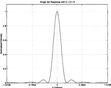
Figure 2.7 shows the PSF for d = 0.1 m and X = 0.03 m

The PSF has a clearly discernible main lobe and several side lobes that are much smaller in amplitude. The null-to-null beamwidth of the main lobe is

6nn = 2 asin X

d (2.36)

With the given parameters, On, ~ 35*.

Points that are angularly separated by On/2 or more can be discerned from one another. The resolution of the slit is therefore

(46)

resolution= asin (2.37)

The beamwidth decreases as the aperture size is increased relative to the carrier wave-length. As mentioned earlier, the width of the main lobe determines the maximum achiev-able resolution. The side lobes bring ghost images in from outside the main lobe. These ghosts corrupt the constructed image; the lower the relative side lobe level the less effect they will have on the image. Clear, high-resolution images can be obtained if the PSF has a narrow main lobe and low side lobes. Unfortunately, one attribute generally has to be traded with the other.

Single Slit Response with d = 0.1 m

0 .8 . .. . . . .. . . .. . .. .. .. . 0.4 -. ... . .. . 0.2-08 -- -- --- -- - - --1r5708 -07854 0 0.7854 1.5708 6 (radians]

Figure 2.7 Single Slit Aperture Point Spread Function

2.3.2 Single Baseline Sparse Array

The single slit aperture can be thought of as an array of an infinite number of pinhole aper-tures. The simplest interferometer consists of two pinhole aperaper-tures. Let us examine how well an array of two pinholes located a distance d apart, as shown in Figure 2.8, approxi-mates the single slit aperture.

(47)

E(x')

2 2

Figure 2.8 Two Pinhole Amplitude Distribution

The amplitude distribution is given by

E(x') = 8(x' + ) + 8(x' - ) (2.38)

The distance between the two pinholes is referred to as the baseline. Applying the integral part of (2.24) to the source distribution, the PSF is

(x) = 2cos

(

dx (2.39)

Expressed as a function of angle from boresight

(0) = 2cos 7E sin0O (2.40)

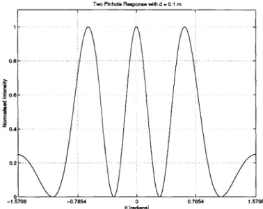
Figure 2.9 shows the PSF for d = 0.1 m and X = 0.03 m .

This PSF does not have a main lobe; all the lobes have equal amplitude. The null-to-null width of the centre lobe is

Onn = 2 asin (2.41)

(48)

0.6

.0

Two Pinhole Response with d = 0.1 m

0

0 [radians]

1.5708

Figure 2.9 Two Pinhole Point Spread Function

This is the same as the null-to-null width obtained with the single slit (2.36). However, the side lobes of the response pattern all have the same amplitude as the main lobe. Since all the lobes have equal amplitude, energy originating from the centre lobe is indistinguish-able from energy originating from the side lobes. The resulting image will contain aliased copies, or ghosts, from the off-centre lobes. Despite having the same resolution as the sin-gle slit aperture, the image quality is significantly worse.

For the general case of 2n apertures distributed evenly across a distance d, the amplitude distribution is n Eeven(x') = (8(x' +

)

+ S - dx' ni ni i = 1 The associated PSF is n

Eeen(O) = 2 cos 9 dsinO6

i = 1

(2.42)

(49)

For the general case of (2n + 1) pinholes distributed evenly across a distance d, the amplitude distribution is n (, dd ni n P Eod~~~~~x)~ = 1(' jx+ +6x-(.4 The associated PSF is n

Eodd(6) = cos) 2+d2 sin (2.45)

i= 1

Taking the limit as n tends to infinity in either (2.43) or (2.45), we obtain the PSF of the slit (2.35).

By adding additional pinholes to the sparse array, the synthesized aperture response will

more closely approach that of the slit, and the quality of the image will improve.

2.3.3 Image Construction using Interferometry

Now that we have seen how the two point-aperture interferometer works we can genera-lise the discussion to an interferometer consisting of an arbitrary number of apertures, which are distributed in two dimensions. In the case where the apertures are distributed across three dimensions, the discussions can be applied by projecting the apertures onto a plane. We turn to Fourier theory for aid in understanding the interferometer.

The discrete Fourier transform acts as a bank of narrowband filters. Given the DFT of a band-limited time-domain signal, and assuming that the sampling frequency is high enough to prevent aliasing, we can reconstruct the time-domain signal with increasing accuracy as the spacing between the filters is decreased. This corresponds to increasing the sampling interval