HAL Id: hal-02089433
https://hal.sorbonne-universite.fr/hal-02089433
Submitted on 3 Apr 2019
HAL is a multi-disciplinary open access
archive for the deposit and dissemination of
sci-entific research documents, whether they are
pub-lished or not. The documents may come from
teaching and research institutions in France or
abroad, or from public or private research centers.
L’archive ouverte pluridisciplinaire HAL, est
destinée au dépôt et à la diffusion de documents
scientifiques de niveau recherche, publiés ou non,
émanant des établissements d’enseignement et de
recherche français ou étrangers, des laboratoires
publics ou privés.
prominence
M. Zapiór, B. Schmieder, P. Mein, N. Mein, N. Labrosse, M. Luna
To cite this version:
M. Zapiór, B. Schmieder, P. Mein, N. Mein, N. Labrosse, et al.. Exploration of long-period oscillations
in an H α prominence. Astronomy and Astrophysics - A&A, EDP Sciences, 2019, 623, pp.A144.
�10.1051/0004-6361/201833614�. �hal-02089433�
Astronomy& Astrophysics manuscript no. 33614 ESO 2019c March 4, 2019
Exploration of long-period oscillations in an H
α
prominence
M. Zapiór
1, B. Schmieder
2, P. Mein
2, N. Mein
2, N. Labrosse
3, and M. Luna
4, 51 Astronomical Institute ASCR, Friˇcova 298, 251 65 Ondˇrejov, Czech Republic
e-mail: maciej.zapior@asu.cas.cz
2 LESIA, Observatoire de Paris, PSL Research University, CNRS Sorbonne Université, Univ. Paris 06, Univ. Paris Diderot, Sorbonne
Paris Cité, 5 place Jules Janssen, Meudon, 92195, France
3 SUPA School of Physics and Astronomy, University of Glasgow, Glasgow, G12 8QQ, UK 4 Instituto de Astrofísica de Canarias, E-38200 La Laguna, Tenerife, Spain
5 Departamento de Astrofísica, Universidad de La Laguna, E-38206 La Laguna, Tenerife, Spain
Received ...; accepted ...
ABSTRACT
Context. In previous work, we studied a prominence which appeared like a tornado in a movie made from 193 Å filtergrams obtained with the Atmospheric Imaging Assembly (AIA) imager aboard the Solar Dynamics Observatory (SDO). The observations in Hα obtained simultaneously during two consecutive sequences of one hour with the Multi-channel Subtractive Double Pass Spectrograph (MSDP) operating at the solar tower in Meudon showed that the cool plasma inside the tornado was not rotating around its vertical axis. Furthermore, the evolution of the Dopplershift pattern suggested the existence of oscillations of periods close to the time-span of each sequence.
Aims. The aim of the present work is to assemble the two sequences of Hα observations as a full data set lasting two hours to confirm the existence of oscillations, and determine their nature.
Methods. After having coaligned the Doppler maps of the two sequences, we use a Scargle periodogram analysis and cosine fitting to compute the periods and the phase of the oscillations in the full data set.
Results. Our analysis confirms the existence of oscillations with periods between 40 and 80 minutes. In the Dopplershift maps, we identify large areas with strong spectral power. In two of them, the oscillations of individual pixels are in phase. However, in the top area of the prominence, the phase is varying slowly, suggesting wave propagation.
Conclusions. We conclude that the prominence does not oscillate as a whole structure but exhibits different areas with their own oscillation periods and characteristics: standing or propagating waves. We discuss the nature of the standing oscillations and the propagating waves. These can be interpreted in terms of gravito-acoustic modes and magnetosonic waves, respectively.
Key words. Sun: filaments, prominences - Sun: oscillations, - Techniques: spectroscopic
1. Introduction
The Solar Dynamics Observatory (SDO; Pesnell et al. 2012) spacecraft, thanks to its high-spatial- and temporal-resolution At-mospheric Imaging Assemblyimager (AIA; Lemen et al. 2012), has evidenced the strong dynamic nature of solar prominences, for example high flows in quasi-vertical structures, rising bub-bles, and rotating, tornado-like structures (Dudík et al. 2012; Orozco Suárez et al. 2012; Wedemeyer et al. 2013; Berger 2014; Su et al. 2014; Levens et al. 2015). Using the Hinode Extreme ul-traviolet Imaging Spectrometer (EIS; Culhane et al. 2007), rota-tion in tornado-like prominences has been suggested from Dopp-lergrams obtained in the 195 Å and 185 Å lines (Su et al. 2014; Levens et al. 2015). These two lines are formed at coronal tem-peratures (log T > 6), and thus these measurements concerned mainly the envelope or prominence-corona transition region. It is therefore important to also analyse the behaviour of the cool plasma inside tornadoes.
Spectro-polarimetric observations of tornadoes are rare be-cause of the long exposure time needed to scan the whole struc-ture with a slit (around 20 min to 1 hour). This problem is ex-acerbated with lines formed at low temperature. Tornadoes have
been observed in optical wavelength range in He i 10830 Å with the Tenerife Infrared Polarimeter (TIP) operating at the Vac-uum Tower Telescope (VTT) ( e.g. Orozco Suárez et al. 2012; Martínez González et al. 2016), in the He i D3 line by the Téle-scope Héliographique pour l’Etude du Magnétisme et des Insta-bilités Solaires (THEMIS, the French telescope in the Canary Islands), and in Hα at the Meudon solar tower (Schmieder et al. 2017). The cadence of the acquisition of the data at the VTT and in THEMIS is too slow to follow the fast evolution of the Dopplershift pattern in the whole structure. Martínez González et al. (2016) used the scanning mode and obtained four consec-utive spectro-polarimetric scans in four hours. They could not find any coherent behaviour between the two successive scans and concluded that if rotation exists it must be intermittent and last less than one hour. This can be explained by the paper of Schmieder et al. (2017). These authors reported observations of a tornado obtained with the Multi-channel Subtractive Double Pass spectrograph (MSDP) operating at the Meudon solar tower. The MSDP has the capability to observe a FOV in nine wave-lengths along the Hα profile simultaneously. With this instru-ment, Dopplershift maps have been registered with a cadence of two per minute, making it possible to follow the fast evolution
Article number, page 1 of 10
of the Dopplershift pattern. Therefore the authors were able to show that large blueshift cells become large redshift cells in a quasi periodic manner.
Using data provided by the Hinode/SOT spectrometer work-ing in the Hα line and by the Interface Region Imagwork-ing Spec-trograph (IRIS; De Pontieu et al. 2014) working in the doublet of Mg ii, Kucera et al. (2018) reported observations of tornadoes. These authors also found that there were Doppler shifts at certain times and locations. The Doppler shifts were however transitory and localised and could be the result of oscillations or motions of particular features along the line of sight. On the other hand, Yang et al. (2018) analysed two tornadoes in Mg ii lines with a very narrow FOV and observed blueshifts and redshifts adjacent to each other over a timescale of two and a half hours. They in-terpreted this as evidence that the tornadoes were rotating. The narrow FOV however covered only a part of the tornado, and it is not clear whether or not this FOV was representative of all the structure motions.
On the theoretical side, Luna et al. (2015) presented an MHD model based on a vertical cylinder with a vertical field along its central axis, and a helical field at the periphery; it is dif-ficult to model such a structure and obtain the corresponding Stokes parameters. However, polarimetric measurements from THEMIS did not indicate the existence of vertical structures. THEMIS has been observing prominences during several inter-national campaigns with the MulTi-Raies (MTR) mode (López Ariste et al. 2000). More than 200 prominences have been ob-served in the He i D3 line. Both statistics (López Ariste 2015) and case studies have been published (Schmieder et al. 2013, 2014). The main result was that the magnetic field is mainly hor-izontal in prominences. Recently, the magnetic field of several tornado-like structures has been analysed and the histograms of the inclination of the magnetic field showed a dominant horizon-tal component of the field and two secondary peaks which have been interpreted up to now as the presence of microturbulence and not a vertical magnetic field (Schmieder et al. 2015; Levens et al. 2016b).
Several authors consider tornadoes to be the legs of promi-nences (Wedemeyer et al. 2013; Levens et al. 2016a). Many static models consider legs or barbs of prominences to be the accumulation of dips (Aulanier & Demoulin 1998; Dudík et al. 2008; Heinzel & Anzer 1999; Mackay et al. 2010; Gunár et al. 2018). Simulations of filament formation by condensation con-firm that cool plasma would be located in the dips of magnetic field lines (Antiochos et al. 1999; Karpen et al. 2001; Luna et al. 2012; Xia et al. 2014).
Waves and oscillations are very common in solar promi-nences and have been reported for many years (see review by Arregui et al. 2018). Several tornado studies interpreted the Doppler signatures and the apparent motions as oscillations in-stead of true rotations. Panasenco et al. (2014) explained the motions detected in AIA as a combination of horizontal os-cillations and counterstreaming flows. These motions give the impression of apparent rotation in the plane-of-the-sky (POS). Mghebrishvili et al. (2015) observed a tornado during the erup-tion of the prominence. The authors suggested that the observed motions could be explained as kink oscillations in a vertical tube. In the model of these latter authors, the tube is the heavy promi-nence mass suspended in the horizontal dips of a quadrupolar magnetic structure. Schmieder et al. (2017) reported Doppler measurements in a tornado structure and concluded that the ob-served motions resulted from the combination of horizontal os-cillations with the global motion of the prominence associated with a parasitic polarity close to the prominence footpoint. In
all cases the motions can be associated with quasi-hourly os-cillations that are very common in solar prominences (see, e.g. Luna et al. 2018). In the current work, we revisit the work of Schmieder et al. (2017) in an attempt to disentangle the proper motions of the filament from the periodic motions associated with the oscillations.
In this paper we select a tornado observed in the 193 Å fil-ter of SDO/AIA on September 24, 2013. The rotation of this prominence can be visualised in the SDO/AIA 193 Å movies (available on https://helioviewer.org). We revisit the ob-servations of the prominence obtained at the Meudon solar tower with the MSDP and already analysed in Paper I (Schmieder et al. 2017). Section 2 presents the data
and Sect. 3 introduces the Scargle method compared to the cosine fit to analyse the oscillations. We derive the character-istics of the oscillations: period, amplitude, phase, and propa-gation. Finally we discuss the possible modes of the propagat-ing waves (Section 4). We find two large areas in the promi-nence with standing waves compatible with gravito-acoustic os-cillations. In addition, a third region shows propagating waves emanating from one of the oscillating regions. These waves are consistent with magnetosonic modes propagating in the vertical direction.
2. H
α
dataThe present tornado-like structure was observed as a filament a few days before in the survey image of Meudon (Schmieder et al. 2014).
2.1. MSDP observations
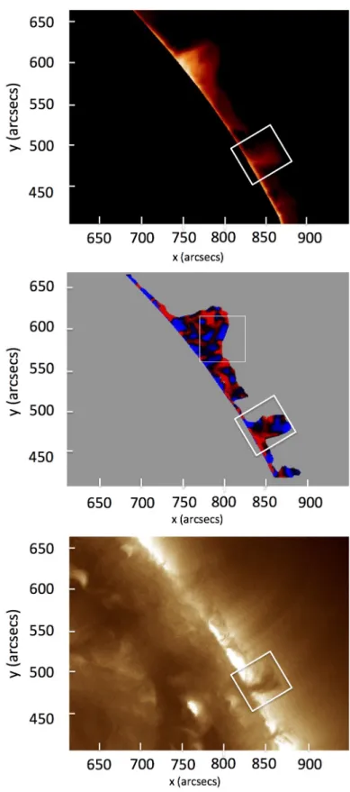
Time sequences of Hα MSDP observations obtained at the Meudon Solar Tower on September 24, 2013, have already been analysed for different purposes (Schmieder et al. 2014; Heinzel et al. 2015). In these two former papers only the quiet part of the prominence located in the northern part of the FOV was under study; this was also in the FOV of IRIS. The southern part of the prominence was analysed later and classified as an AIA tornado (Paper I). Here we focus our study on the Hα data of the tor-nado structure located in the south and indicated by a white box in Figure 1. Two sequences of observations with a cadence of two images per minute were obtained and last approximatively 1 hour each: from 12:06 UT to 12:53 UT and from 13:04 UT to 14:02 UT.
2.2. Dopplershifts
MSDP observations consist of nine images obtained in nine channels of 465 arcsec × 60 arcsec. The wavelength step cor-responding to the same solar point in two consecutive channels is 0.3 Å. Calibrations and line profiles were obtained from the usual MSDP software (Mein 1991).
The zero Dopplershift is determined using a mean value across the full prominence available in the FOV, including the upper part of the observed region (Figure 1). Indeed, taking av-erage values across the solar disc would not take into account, in particular, the departures between telluric line effects on absorp-tion and emission profiles.
The scattering effects are corrected as follows. The intensity of prominence profiles is negligible in the extreme channels 1 and 9 of the MSDP. These channels can be used in each pixel of the prominence to estimate the far wings of the scattered light
M. Zapiór et al.: Exploration of long-period oscillations in an Hα prominence
coming from the solar disc. A simple normalization of the disc spectrum then allows to estimate the full scattered light profile. Because the limb is not parallel to the direction of dispersion in the spectrograph, some additional uncorrected scattered light may occur in points close to the limb, but this should not affect the computation of oscillations appreciably.
To estimate error bars for velocities, we can distinguish two kinds of errors. The first one is the data noise from CCD pixels. In Paper I, we obtained estimates from 0.2 to 0.3 km/s by us-ing noise effects in intensity measurements and departures from velocities observed in neighbouring points. The second one con-cerns errors due to interpolation of line profiles. They depend mainly on slow drifts of the prominence in the FOV during time sequences, and result in stochastic wavelength drifts in each so-lar point. A comparison between cubic and Gaussian interpola-tions was used in paper I to get estimates. The result was 0.3 km/s. Error bars due to both kinds of errors can be estimated at ± 0.5 km/s.
3. Oscillations
We focus the study on the Dopplershifts computed in the tornado shown in the white box in Figure 1. In Paper I each sequence was considered independently because of the gap of 15 minutes between them. The periodicity of the oscillations that were re-ported by looking at the variation of the Dopplershift in individ-ual pixels was close to the time interval of each sequence (around 60 minutes). Here we add the two sequences using a 2D Fourier correlation function and obtain one data cube of Dopplershift maps for a time-span of two hours. Based on the oscillatory be-haviour of each sequence taken individually, the use of Scargle periodograms, which compute the period of oscillations in the case of unevenly spaced data with gaps, is appropriate.
3.1. Method
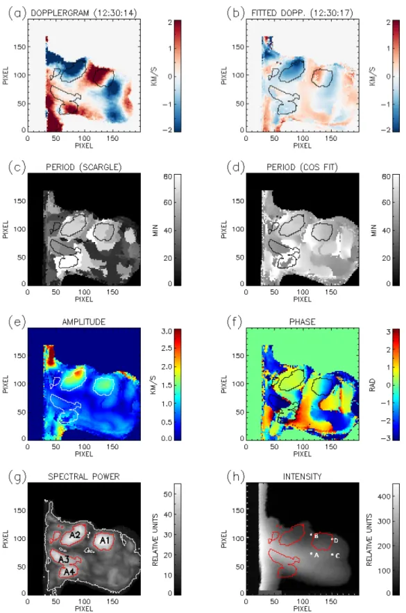
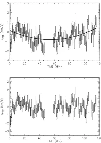
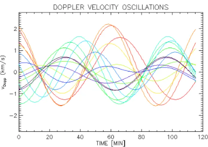
From the series of Dopplergrams (see Figure 2a) we calculated the evolution of the Doppler velocity for each pixel in the field of view (FOV) independently. The top panel of Figure 3 shows the Doppler velocity in one pixel example. We fit each individual pixel signal by a cosine curve, plus a second-order polynomial function to detrend the proper motions of the prominence. The bottom panel of Figure 3 presents the detrended signal, clearly showing the oscillatory behaviour. This trend function filters out motions associated with oscillation periods longer than the se-quence duration and reduces instrumental effects like thermal dilatation of the spectrograph devices. Figure 4 shows the de-trended Doppler velocities in four selected pixels and their re-spective periodograms. The selected pixels are shown in Figure 2h. We verified that the detrending has no substantial influence throughout the FOV.
Subsequently, for all pixels, we calculate the Scargle odogram (Scargle 1982) which allows the identification of peri-odic signals in unevenly spaced data with gaps. Another method to deal with this kind of data is the discrete Fourier transform (DFT; Kurtz 1985; Deeming 1975). A DFT however has two disadvantages: high noise in a periodogram and spectral leak-age. Scargle’s formula suppresses these effects by introducing a new definition of the periodogram:
PX(ω)= 1 2 hP jXjcos ω(tj−τ) i2 P jcos2ω(tj−τ) + hP jXjsin ω(tj−τ) i2 P jsin 2ω(t j−τ) ,
Fig. 1. Prominence observed on September 24, 2013, at 12:22 UT with the MSDP operating on the solar tower in Meudon and with SDO/AIA. Top panel: Hα intensity, middle panel: Hα Dopplershift map, bottom panel: AIA 193 Å image. The white box indicates the ‘tornado’ (ap-proximate FOV of Figure 2).
where Xj are data points observed at times tj for { j= 1, 2, . . . , N0}, τ is defined by tan(2ωτ)= X j sin 2ωtj / X j cos 2ωtj ,
Fig. 2. Oscillatory features of the tornado prominence (the FOV is shown in Figure 1 inside the white box). (a) Snapshot of the Dopplergram movie at 12:30 UT. (b) Example of the fitted Dopplergram at 12:30 UT. (c) Period value from periodogram analysis. (d) Period value from cosine curve approximation. (e) Amplitude value from cosine curve approximation. (f) Phase from cosine curve approximation (note that phase -π is equal to π radians); (g) Spectral power from periodogram analysis; white line limits areas with FAP=1%, red line limits areas with a spectral power higher than 32, which is also overplotted in all panels with black, white, or red lines. A1, A2, and A3 indicate areas where the mean oscillatory parameters presented in Table 1 are calculated. (h) Hα intensity image with the positions of selected pixels taken as samples of Doppler signal shown in Figure 4. Colour-bars give units of distribution of parameters. We note that 1 pixel= 0.25 arcsec. The temporal evolution of the Doppler maps in panels (a) and (b) is available in a movie online.
M. Zapiór et al.: Exploration of long-period oscillations in an Hα prominence
Fig. 3. Example of Doppler velocity signal for pixel A with fitted parabola (top). The signal with subtracted parabola is presented in the bottom panel. The error bar is ± 0.5 km s−1. The gap in the data is
between the two sequences observed by the MSDP.
and ω is calculated for the so-called natural set of frequencies: ωn= 2πn/T {n = −N0/2, . . . , +N0/2}.
Additionally Scargle (1982) defines the false-alarm probability (FAP):
P(FAP)= − lnh1 − (1 − FAP)1/Ni ,
where N = N0/2. With this definition, P(FAP) gives a power level of such a value that the periodogram peak above P(FAP) is caused by pure noise only with a probability equal to the FAP. The FAP may be interpreted as a confidence level equal to 1 − FAP.
We constructed a map of periods corresponding to the max-imum peak in the periodograms calculated with the Scargle for-mula in the observed prominence (Fig. 2c). This map shows large areas with the same or a similar period. The range of pe-riods is mainly between 40 and 80 minutes. Figure 2g presents the distribution of the maximum spectral power for individual pixels, showing that in almost the whole observed prominence, the FAP level is below 1%. For all pixels we then fitted a cosine function (solid lines in left panels of Fig. 4):
Acos 2π Pt+ φ
! ,
where A is amplitude, P is period, φ is phase shift. We used a pro-cedure mpfit, which performs robust non-linear least squares curve fitting (Markwardt 2009). We limited the range of periods to 40–80 minutes because this range covers the most prominent periods. From the cosine curve fitting we derived a set of param-eters: A, P, and φ, as immediately above. The spatial distribution of these parameters is shown respectively in Figs. 2(d–f). Hav-ing a continuous variation of Doppler signal (from curve fittHav-ing) for all pixels, we constructed the 2D time evolution of the fitted functions. One 2D map for a particular time may be treated as a “fitted” or “approximated” Dopplergram. The time evolution of raw and “fitted” Dopplergrams is presented in the animation available in the electronic version of the manuscript.
3.2. Results
We discuss the results presented in the seven panels of Figure 2 in the frame of defining the nature of the oscillations. Panels (a) and (b) are snapshots of the movie showing the raw Doppler-shifts and the fitted Doppler Doppler-shifts, respectively, for one time, panel (c) shows the Scargle periodogram, panel (d) shows the period from cosine fitting, panels (e, f, g) present the amplitude, the phase, and the spectral power from the cosine fitting, and panel (h) shows the Hα intensity.
3.2.1. Periods
We detect oscillatory motions with periods between 5 and 80 minutes (Figure 2c). The shorter periods (5 to 40 minutes) have a local significance level of around 99%; they last only two to four times their periods and are visible in small areas. It would be interesting to find out where and when they occur, but this is beyond the scope of this study. Here, we concentrate our work on the long periods between 40 and 80 minutes which were al-ready detected in Paper I. We find that the prominence does not oscillate as a block at these long periods. We identify four main oscillatory areas with a high spectral power (see Figure 2g and Table 1). We select these four areas with high spectral power and overplot their contours on all the panels of Figure 2. For each
Fig. 4. (left) Doppler signal for the selected pixels marked in Fig. 2(h) and (right) corresponding Scargle periodograms of the signal. (+) symbols correspond to data, solid line to a cosine fit. Dashed line represents FAP=1%, dotted line represents FAP=5%. On the left panels, the P value gives the period of the fitted cosine curve in minutes. The error bar is equal ± 0.5 km s−1.
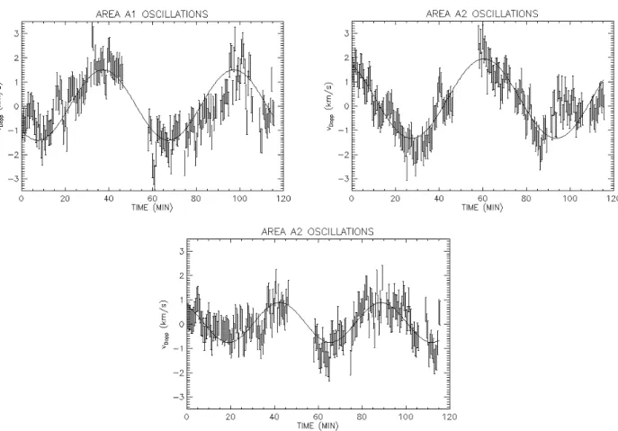
area, we calculate the mean value of the oscillatory parameters (see Table 1). The value of the spectral power in relative units is around 40. The mean oscillation period for areas A1 and A2 is close to 65 minutes with the two methods (Scargle and cosine fit methods). For area A3 we obtain a value of 45 minutes. We
ex-clude area A4 from further analysis because of the non-uniform pattern in period, amplitude, and phase distribution, which is a hint of the bad fit of the cosine curve due to high noise. Addi-tionally, the periods calculated using the two methods are sig-nificantly different. We may note that a similar period value of
M. Zapiór et al.: Exploration of long-period oscillations in an Hα prominence
65 minutes is commonly observed for longitudinal oscillations in prominences (Luna et al. 2018). In areas A1, A2, and A3, the period is nearly uniform (Figure 2c). The mean amplitude of the oscillations is between 0.70 km s−1and 1.43 km s−1, values larger than the estimation of the error bars. However, higher am-plitude values are present in the selected areas, reaching locally 3 km s−1(Figure 2e). We notice another region with even higher amplitude located near the pixel coordinates (x=40, y=150), but the signal has a relatively low spectral power value and is too small to be treated as an oscillating feature.
3.2.2. Phase
Fitted phase is presented in Figure 2f. In areas A2 and A3 at the bottom of the prominence the phase has the same value in each area.
Additionally, in each of these two regions the period values are very similar (see Figs. 2c and 2d), and the spectral power reaches local peaks (see Figure 2g).
On the contrary, in area A1 the period and amplitude are sim-ilar but the phase does not have a uniform value; it shows a con-tinuous transition between -π and 0 radians. This may be inter-preted as the passage of a wavefront of a MHD wave (Schmieder et al. 2013; Ofman et al. 2015). The colour gradient gives the di-rection of the propagation of the wave in the POS. This is clearly visible in the animation of the Figure 2b available in the elec-tronic version of the journal.
3.2.3. Wave propagation
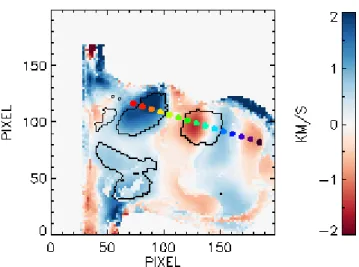
For a more detailed study of the wave propagation, we con-structed a time-distance diagram. In Figure 5 we present a Doppler snapshot with a superimposed path, along which we calculate the time-distance diagram (Figure 6).
Let us first comment on the accuracy of the data. By compar-ing Fig. 3 of Paper I and our Fig. 5 we see that the direction of the path of the latter is close to the direction of constant wavelengths in the MSDP channels. This implies that the mean velocity er-rors due to interpolation are similar along the path in Fig. 5, the latter being used to calculate the velocities in Fig. 6.
Three different patterns in the time-distance diagram can be distinguished in Fig. 6. The first pattern is from 0 to ∼7000 km along the path from left to right (represented by red to yellow points) and corresponds to the area A2. There is a small phase shift in A2 associated to a possible wave propagation in the right panel of the figure. However, looking at the left panel, we clearly see a blue and red pattern associated to standing modes. The small phase shifts could be associated to a possible artifact of the method used. For this reason we interpret the periodic motions in A2 as rigid oscillations. The oscillations are mainly in phase, which is visible in Fig. 7, where variations of the Doppler veloc-ity for the selected pixels along the path are presented. Curves with red to yellow colours correspond to area A2. The second feature is from ∼8000 to ∼17000 km and corresponds to area A1 and its surroundings. The oscillations are propagating along the path – this is visible in Fig. 7 from the coloured curves (from green to purple) which are consecutively shifted in phase. From the calculation of the position of the same phase (see Figure 6), we estimate the phase velocity in this area to be 4.8 ± 1.2 km s−1. We must keep in mind that this value is only a lower limit because of projection effects. AIA 193 and AIA 304 movies (available on https://helioviewer.org), where the whole promi-nence system was visible as a long filament on the solar disc,
show that two or three days before September 24, the filament structure had a C shape and the analysed region was located in the meridional part of the system. This suggests that the analysed prominence is seen edge-on. This allows us to conclude that the real phase velocity is not much higher than calculated. The last pattern is visible from ∼19000 to ∼22000 km and can be treated as a standing wave, but it does not correspond to any area with high spectral power (see Figure 2g).
4. Discussion and conclusion
A tornado-like prominence (exhibiting apparent rotational mo-tions in AIA 193 Å movie) was followed for two hours at the Meudon Solar Tower with the MSDP spectrograph in Hα. A par-tial analysis of the same data was presented in Paper I. We study again the spatial variation of the Hα Doppler shifts in the promi-nence in order to see if we can detect a rotation motion in the cool plasma (104K).
As in Paper I we do not find any sign of tornado-like rota-tion, which means that no systematic red- or blue-shift pattern is present in opposite sides of the prominence vertical axis over large periods of time, as reported by Su et al. (2014), Levens et al. (2015), and Yang et al. (2018) from the analysis of EIS and IRIS observations of different tornadoes.
In this work, we confirm the presence of oscillatory motions with periods between 40 and 80 minutes already identified in Pa-per I. We extend the analysis by using the Scargle Pa-periodogram method and find that the prominence does not oscillate at the same frequency as a block. We identify three main oscillatory areas, A1, A2, and A3, which are disconnected. The oscilla-tions are coherent inside areas A2 and A3. In area A1 the phase changes in a continuous way suggesting a propagating wave.
With the MSDP we have information on the 2D oscillating pattern and we avoid detecting false oscillations caused by slit shift in slit-spectrographs (Balthasar et al. 1993; Zapiór et al. 2015).
The oscillations in regions A2 and A3 can be interpreted as normal modes of the prominence structure where a large part of the structure oscillates coherently. Several works considered the normal modes of prominences, modelling them as a plasma slab supported in a horizontal magnetic field (e.g., Joarder & Roberts 1992, 1993; Oliver et al. 1993). These latter authors found MHD modes of vibration of the prominence with periods of around one hour with horizontal velocities, in agreement with our ob-servations. All of these modes are internal slow modes. In these modes the period is dictated essentially by the phase speed and the width of the prominence plasma slab. More recently, Luna & Karpen (2012) and Luna et al. (2012) found that longitudinal oscillations are strongly influenced by the curvature of the mag-netic field. The resulting generalised modes are called gravito-acoustic modes or pendulum modes. The authors found that in prominence conditions the gravity projected along the field lines dominates over the gas-pressure gradients as the restoring force. The period of the oscillations depends exclusively on the radius of curvature of the dipped field lines, R. Recent 2D and 3D nu-merical simulations have found that the horizontal and hourly oscillations are in agreement with the pendulum model (Luna et al. 2016; Zhou et al. 2018) and this mode is excited after an external perturbation. We can apply the pendulum model expres-sion (Luna & Karpen 2012; Luna et al. 2012),
P= 2π s
R
g, (1)
Fig. 5. Dopplergram snapshot rotated for convenience with superimposed path (colour points) used to calculate time-distance diagram (see Figure 6). The colours of the points correspond to plots in the Fig. 7.
Fig. 6. Time-distance diagrams calculated along the path presented in Fig. 5. Left panel: Detrended data; the white horizontal spaces are due to the lack of data. Right panel: As in left panel but gaps are interpolated by cosine fit with the assumption of the oscillatory trend of the data. Black lines mark positions of the same phase used to calculate the phase velocity. Numbers above lines give the calculated phase velocity at these positions. Table 1. Mean oscillatory parameters calculated for areas with the highest spectral power (see Figure 2).
Area A1 A2 A3 A4
Coordinates [pxl] (130,90) (74,100) (60,70) (70,40) Spectral Power [rel.units] 48.50 41.13 40.45 39.57
Amplitude [km s−1] 1.33 1.43 0.70 0.32 Period(Scargle) [min] 62.68 64.98 45.07 84.19 Period(Cosine fit) [min] 62.31 64.44 45.98 64.20
in the three regions with clear oscillations using the periods shown in Table 1, that is A2-A4. In this expression, g is the
M. Zapiór et al.: Exploration of long-period oscillations in an Hα prominence
Fig. 7. Time variation of the Doppler velocity along the selected path. The colours correspond to positions along the path shown in Fig. 5.
53, and 103 Mm respectively, calculated using periods from the cosine fit of the table. In Schmieder et al. (2017) we argued that the pendulum model requires a very rigid magnetic field. How-ever, in light of the recent realistic 3D numerical simulations by Zhou et al. (2018), we do not find a reason to reject this model.
In region A1, a propagating wave is observed with a phase speed between 4.9 and 7.3 km s−1and a period of approximately 62 minutes. This is similar to the observation by Terradas et al. (2002) in a limb prominence. However, these authors found a complex pattern of wave propagation in a large portion of the prominence. This contrasts with our observation where the prop-agation is almost vertical. Vertical propprop-agation of waves has al-ready been observed by Schmieder et al. (2013), but with much smaller periods of a few minutes associated to magnetosonic waves. The restoring force in these waves is the gas and mag-netic pressure gradients perpendicular to the magmag-netic field. The authors suggested that the waves were driven by photospheric or chromospheric oscillations (see also Ofman et al. 2015). Mash-nich et al. (2009a) and MashMash-nich et al. (2009b) studied simulta-neous Doppler velocities in filaments and the photosphere under-neath, finding quasi-hourly oscillations in both with good spatial correlation. This suggests that it is possible to drive quasi-hourly oscillations in prominences from below.
Alternatively to wave propagation, the observed motions can also be interpreted in terms of standing waves or oscil-lations. Kaneko et al. (2015) found that the Alfvén- and/or slow-continuum in prominence structures can create the illu-sion of wave propagation across the magnetic field. This phe-nomenon can be erroneously interpreted as fast magnetosonic waves. The motion is apparent because there is no propagation of energy across magnetic surfaces. These apparent waves have been called superslow waves. Luna et al. (2016) studied longi-tudinal oscillations associated with the gravito-acoustic modes and the authors found a similar behaviour with horizontal oscil-lations giving the impression of a vertical propagation. This phe-nomenon is associated with oscillations along the magnetic field where the characteristic oscillation periods depend on the param-eters of each field line. In these oscillations, the characteristic pe-riods form a continuum with smooth variations in a prominence structure. In this situation, the plasma in each field line oscillates with its own period producing phase differences that give the impression of propagation perpendicular to the magnetic field. Raes et al. (2017) studied observationally superslow oscillations detected in a filament. Combining the observations with di
ffer-ent models they performed seismology with superslow oscilla-tions for the first time. They found an apparent wave velocity of 4-14 km s−1 and periods of 59 - 76 minutes similar to our observations. The authors used the pendulum model of Luna & Karpen (2012) in a simplified structure to show that it is possible to obtain information on magnetic field structure using super-slow waves and determine the radius of curvature of field lines that support the prominence but also the position of the centre of the flux rope. However, according to the calculations of Raes et al. (2017), the phase speed decreases with time, which contra-dicts our findings.
In this work, we demonstrate that rotational movements in prominence tornadoes are apparent. These motions are consis-tent with prominence oscillations. The oscillations have a com-plex spatial distribution with three different regions showing a strong spectral power. In regions A2 and A3 we find standing quasi-hourly oscillations consistent with slow normal modes or with gravito-acoustic mode. In contrast, propagating waves are found in A1 travelling in the vertical direction. A possible expla-nation is that A2 drives the waves in A1 in some kind of wave leakage. Our observations are very similar to those of Terradas et al. (2002) who found large areas in the prominence with stand-ing waves and areas with propagatstand-ing waves. The authors found that the propagating waves were generated in a narrow region with standing waves. In our region A1, the waves propagate in the vertical direction, almost perpendicular to the typically hor-izontal prominence magnetic field. These waves can be inter-preted in terms of magnetosonic waves. New long time series observations with the MSDP and other imaging spectrographs (e.g. Fabry-Pérot type) should be done to study how frequently this kind of oscillation in prominences is detected.
Acknowledgements. We would like to thank the team of MSDP for acquiring the observations (Regis Le Cocguen and Daniel Crussaire). MZ is supported by the project RVO:67985815. NL acknowledges support from STFC grant ST/P000533/1. ML acknowledges the support by the Spanish Ministry of Econ-omy and Competitiveness (MINECO) through projects AYA2014- 55078-P and under the 2015 Severo Ochoa Program MINECO SEV-2015-0548. ML also ac-knowledges the support by ISSI of the team 413 on “Large-Amplitude Oscil-lations as a Probe of Quiescent and Erupting Solar Prominences”. This work was initiated during meetings of the International Team "Solving the prominence paradox" organized by NL, and support from the International Space Science In-stitute is gratefully acknowledged.
References
Antiochos, S. K., MacNeice, P. J., Spicer, D. S., & Klimchuk, J. A. 1999, ApJ, 512, 985
Arregui, I., Oliver, R., & Ballester, J. L. 2018, Living Reviews in Solar Physics, 15, 3
Aulanier, G. & Demoulin, P. 1998, A&A, 329, 1125
Balthasar, H., Wiehr, E., Schleicher, H., & Wohl, H. 1993, A&A, 277, 635 Berger, T. 2014, in IAU Symposium, Vol. 300, IAU Symposium, ed.
B. Schmieder, J.-M. Malherbe, & S. T. Wu, 15–29
Culhane, J. L., Harra, L. K., James, A. M., et al. 2007, Sol. Phys., 243, 19 De Pontieu, B., Title, A. M., Lemen, J. R., et al. 2014, Sol. Phys., 289, 2733 Deeming, T. J. 1975, Ap&SS, 36, 137
Dudík, J., Aulanier, G., Schmieder, B., Bommier, V., & Roudier, T. 2008, Sol. Phys., 248, 29
Dudík, J., Aulanier, G., Schmieder, B., Zapiór, M., & Heinzel, P. 2012, ApJ, 761, 9
Gunár, S., Dudík, J., Aulanier, G., Schmieder, B., & Heinzel, P. 2018, ApJ, 867, 115
Heinzel, P. & Anzer, U. 1999, Sol. Phys., 184, 103
Heinzel, P., Schmieder, B., Mein, N., & Gunár, S. 2015, ApJ, 800, L13 Joarder, P. S. & Roberts, B. 1992, Astronomy and Astrophysics (ISSN
0004-6361), 256, 264
Joarder, P. S. & Roberts, B. 1993, Astronomy and Astrophysics, 277, 225 Kaneko, T., Goossens, M., Soler, R., et al. 2015, The Astrophysical Journal, 812,
121
Fig. 8. Oscillations of the areas with maximum power spectrum. The error bars of the data are of the order of 0.5 km s−1; solid line - cosine fit.
Karpen, J. T., Antiochos, S. K., Hohensee, M., Klimchuk, J. A., & MacNeice, P. J. 2001, ApJ, 553, L85
Kucera, T. A., Ofman, L., & Tarbell, T. D. 2018, ApJ, 859, 121 Kurtz, D. W. 1985, MNRAS, 213, 773
Lemen, J. R., Title, A. M., Akin, D. J., et al. 2012, Sol. Phys., 275, 17 Levens, P. J., Labrosse, N., Fletcher, L., & Schmieder, B. 2015, A&A, 582, A27 Levens, P. J., Schmieder, B., Labrosse, N., & López Ariste, A. 2016a, ApJ, 818,
31
Levens, P. J., Schmieder, B., López Ariste, A., et al. 2016b, ApJ, 826, 164 López Ariste, A. 2015, in IAU Symposium, Vol. 207, IAU Symposium, ed. K. N.
Nagendra, S. Bagnulo, R. Centeno, & M. Jesús Martínez González, 275–281 López Ariste, A., Rayrole, J., & Semel, M. 2000, A&AS, 142, 137
Luna, M., Díaz, A. J., & Karpen, J. 2012, The Astrophysical Journal, 757, 98 Luna, M. & Karpen, J. 2012, The Astrophysical Journal, 750, L1
Luna, M., Karpen, J., Ballester, J. L., et al. 2018, ApJS, 236, 35 Luna, M., Karpen, J. T., & DeVore, C. R. 2012, ApJ, 746, 30
Luna, M., Moreno-Insertis, F., & Priest, E. 2015, The Astrophysical Journal Let-ters, 808, L23
Luna, M., Terradas, J., Khomenko, E., Collados, M., & Vicente, A. d. 2016, The Astrophysical Journal, 817, 157
Mackay, D. H., Karpen, J. T., Ballester, J. L., Schmieder, B., & Aulanier, G. 2010, Space Sci. Rev., 151, 333
Markwardt, C. B. 2009, in Astronomical Society of the Pacific Conference Se-ries, Vol. 411, Astronomical Data Analysis Software and Systems XVIII, ed. D. A. Bohlender, D. Durand, & P. Dowler, 251
Martínez González, M. J., Asensio Ramos, A., Arregui, I., et al. 2016, ApJ, 825, 119
Mashnich, G. P., Bashkirtsev, V. S., & Khlystova, A. I. 2009a, Geomagnetism and Aeronomy, 49, 891
Mashnich, G. P., Bashkirtsev, V. S., & Khlystova, A. I. 2009b, Astronomy Let-ters, 35, 253
Mein, P. 1991, A&A, 248, 669
Mghebrishvili, I., Zaqarashvili, T. V., Kukhianidze, V., et al. 2015, ApJ, 810, 89 Ofman, L., Knizhnik, K., Kucera, T., & Schmieder, B. 2015, ApJ, 813, 124 Oliver, R., Ballester, J. L., Hood, A. W., & Priest, E. R. 1993, The Astrophysical
Journal, 409, 809
Orozco Suárez, D., Asensio Ramos, A., & Trujillo Bueno, J. 2012, ApJ, 761, L25
Panasenco, O., Martin, S. F., & Velli, M. 2014, Sol. Phys., 289, 603
Pesnell, W. D., Thompson, B. J., & Chamberlin, P. C. 2012, Sol. Phys., 275, 3 Raes, J. O., Van Doorsselaere, T., Baes, M., & Wright, A. N. 2017, Astronomy
and Astrophysics, 602, A75 Scargle, J. D. 1982, ApJ, 263, 835
Schmieder, B., Kucera, T. A., Knizhnik, K., et al. 2013, ApJ, 777, 108 Schmieder, B., López Ariste, A., Levens, P., Labrosse, N., & Dalmasse, K. 2015,
in IAU Symposium, Vol. 305, IAU Symposium, ed. K. N. Nagendra, S. Bag-nulo, R. Centeno, & M. Jesús Martínez González, 275–281
Schmieder, B., Mein, P., Mein, N., et al. 2017, A&A, 597, A109 Schmieder, B., Tian, H., Kucera, T., et al. 2014, A&A, 569, A85 Su, Y., Gömöry, P., Veronig, A., et al. 2014, ApJ, 785, L2
Terradas, J., Molowny-Horas, R., Wiehr, E., et al. 2002, Astronomy and Astro-physics, 393, 637
Wedemeyer, S., Scullion, E., Rouppe van der Voort, L., Bosnjak, A., & Antolin, P. 2013, ApJ, 774, 123
Xia, C., Keppens, R., Antolin, P., & Porth, O. 2014, ApJ, 792, L38 Yang, Z., Tian, H., Peter, H., et al. 2018, ApJ, 852, 79
Zapiór, M., Kotrˇc, P., Rudawy, P., & Oliver, R. 2015, Sol. Phys., 290, 1647 Zhou, Y.-H., Xia, C., Keppens, R., Fang, C., & Chen, P. F. 2018, The