Active noise cancellation in a suspended interferometer
The MIT Faculty has made this article openly available.
Please share
how this access benefits you. Your story matters.
Citation
Driggers, Jennifer C., Matthew Evans, Keenan Pepper, and Rana
Adhikari. “Active Noise Cancellation in a Suspended Interferometer.”
Review of Scientific Instruments 83, no. 2 (2012): 024501.
As Published
http://dx.doi.org/10.1063/1.3675891
Publisher
American Institute of Physics (AIP)
Version
Original manuscript
Citable link
http://hdl.handle.net/1721.1/88408
Terms of Use
Creative Commons Attribution-Noncommercial-Share Alike
Jennifer C. Driggers,1Matthew Evans,2 Keenan Pepper,3 and Rana Adhikari1
1)
LIGO Laboratory, California Institute of Technology, Pasadena, CA 91125a)
2)
LIGO Laboratory, Massachusetts Institute of Technology, Cambridge, MA 02139
3)University of California, Berkeley, Berkeley, CA 94720
(Dated: 13 December 2011)
We demonstrate feed-forward vibration isolation on a suspended Fabry-Perot interferometer using Wiener filtering and a variant of the common Least Mean Square (LMS) adaptive filter algorithm. We compare the experimental results with theoretical estimates of the cancellation efficiency. Using data from the recent LIGO Science Run, we also estimate the impact of this technique on full scale gravitational wave interferometers. In the future, we expect to use this technique to also remove acoustic, magnetic, and gravitational noise perturbations from the LIGO interferometers. This noise cancellation technique is simple enough to imple-ment in standard laboratory environimple-ments and can be used to improve SNR for a variety of high precision experiments.
PACS numbers: 04.80.Nn, 95.55.Ym, 07.60.Ly, 42.62.Eh
I. INTRODUCTION
The next generation of interferometers for gravitational-wave detection, including the Laser Interferometer Gravitational Wave Observatory (LIGO), will have unprecedented sensitivity to astrophysical events1. At low frequencies (∼10 Hz) it is likely that the displacement noise of the suspended mirrors will be limited at the 10−20 m/√Hz level by fluctuations in the Newtonian gravitational forces2–4. The sources
of the fluctuations are density perturbations in the environment (e.g. seismic and acoustic) and mechanical vibrations of the nearby experimental apparatus. While care will be taken to mitigate the sources of all of these fluctuations, further reductions of this Newtonian noise may be made by carefully measuring the source terms and subtracting them from the data stream (offline) or in hardware by applying cancellation forces to the mirror.
To demonstrate the efficacy of this technique, we demonstrate below that offline subtraction of seismic noise can be done using static Wiener filtering based on an array of seismic sensors. The online adaptive sub-traction is also shown to approach the ’optimal’ Wiener limit5. Through nonlinear processes, seismic noise
be-low 10 Hz has been shown to limit the performance of gravitational-wave detectors. This technique will prove to be of substantial value in reducing the non-stationarity of the detectors.
II. STATIC WIENER FILTERING
To find a linear filter that will improve a chosen signal, we must first define what it means to ’improve’ the signal. The figure of merit (ξ) that we use for calculating the
a)Electronic mail: [email protected]
Wiener filters in this case is the expectation value of the square of the error signal (~e), where the error signal is defined as the difference between the target signal to be minimized and the estimate of that signal calculated from the filtered witness channels.
ξ ≡ E[e2(n)] = E[d2(n)] − 2 ~wTp + ~wTR ~w (1) Here, E[∗] indicates the expectation value of ∗, ~w rep-resents the tap weights of the filter, d(n) is the target signal which we would like to minimize, ~p is the cross-correlation vector between the witness and target signals, and R is the autocorrelation matrix for the witness chan-nels. When we solve Eq. 1 by setting
dξ dwi
= 0 (2)
we find
R ~woptimum= ~p (3)
Eq. 3 finds the FIR (Finite Impulse Response) filter co-efficients which minimize the RMS of the error ~e by opti-mizing the estimate of the transfer function between the witness sensors and the target signal. Since the matrix R is Block Toeplitz, we take advantage of the Levinson-Durbin6method of solving problems of the form ~b = M~a,
where M is a Toeplitz matrix. The Levinson method is considered weakly stable, as it is susceptible to numerical round-off errors when the matrix is close to degenerate (i.e. two or more witness sensors carry nearly identical information about the noise source). For well conditioned matricies it is much faster than brute force inversion of the matrix7.
The filtered output of the witness signals is y(n) = ~
wT~x and e(n) = d(n) − y(n) = d(n) − ~wT~x is the fil-tered or minimized target signal, where ~x is the indepen-dent witness signal measuring our noise source. This new
2 minimized signal ~e represents what the the disturbance
~
d would be if we were able to subtract the seismic noise before it entered the system.
Since we are using this feed-forward technique to re-duce noise in the length of our cavities, and the cavity length carries gravitational wave information, we must be careful not to subtract the science signal along with the noise. For seismic noise, we are trying to cancel noise below 10 Hz, while the gravitational wave signal band above 10 Hz. Even so, if we use a filter of the same length as the data stream, we could perfectly cancel ev-erything, including seismic noise and gravitational wave information. However given the short length of our filters and the long stretches of data we calculate the subtrac-tion over, the distorsubtrac-tion of the gravitasubtrac-tional wave signals should not be significant.
While the Wiener filtering occurs entirely in the time-domain, we examine plots in the frequency-domain of the filtered and unfiltered signals to determine the level of subtraction achieved. In Section III we describe the Wiener simulations on a cavity in our lab. In Section IV, we make similar estimates for one of the 4 km LIGO interferometers. Finally, in Section V we demonstrate the performance of a real-time seismic noise cancellation system in the lab.
III. WIENER FILTERING AT THE 40M INTERFEROMETER
At our 40 m prototype interferometer8lab at Caltech,
both static Wiener filtering and adaptive filtering algo-rithms have been applied to a suspended Fabry-Perot triangular ring cavity’s feedback signal. We have used 2 G¨uralp CMG-40T seismometers9and several Wilcoxon
731A accelerometers10 as our independent witness
chan-nels (~x in Section II), and the low-frequency feedback signal for the cavity length as the target channel ( ~d in Eq. 1) to reduce.
Figure 1 shows the locations of the witness sensors rel-ative to the cavity mirrors. The mirrors of the cavity are suspended as pendulums with a resonance of ∼1 Hz to mechanically filter high frequency noise, with the sus-pensions sitting on vibration isolation stacks to further isolate the optics from ground motion. The ’stacks’ are a set of 3 legs supporting the optical table on which the mirror sits, with each of the legs consisting of alternating layers of stainless steel masses and elastomer springs11,12. We used Matlab13 to import the data for the length
feedback signal for our cavity, and to construct and apply the Wiener filters. Since the feedback control bandwidth is '50 Hz, the feedback signal can be used as an accurate measure of the seismic disturbance at low frequencies. In Figure 2 we show results of a day-long simulation study. This study was done to determine the length of time we can use a set of static filters before updating. We use 1 hour of data to train and calculate a single Wiener filter, and then apply that filter to 10 minute segments
M2 M1 M3 Accelerometer Seismometer From Laser Output of Cavity
FIG. 1. Locations of seismometers and accelerometers in rela-tion to the cavity mirrors. Round trip length of the triangular cavity is 27 m.
of data for one day, using a 31 second long, 2000 tap filter with a sample rate of 64 Hz. In Figure 2b, we select a few typical traces to illustrate the capabilities of the filter, while in Figure 2a we show the full results as a spectrogram, whitened by normalizing to the spectra during the time the filter was being trained. We see large amounts of noise reduction both at the broad stack peak at ∼3 Hz and around the 16 Hz vertical mode of the mirror pendula.
We also include the noise contributions of our seis-mometers in Figure 3 to demonstrate how close we are able to get to the fundamental limit of Wiener filtering. Since the Wiener filter accepts, as inputs, the signals from the witness sensors (which have true ground motion in-formation plus self-noise of the instruments and noise in the readout electronics), all of these noise contributions are filtered and added back into our data stream, limiting our ability to suppress ground motion below these levels. In Figure 3, we show that the differential ground motion over the length of the cavity is not much larger than the instrument noise of the seismometers. In other words, the ground noise over length of the cavity is strongly corre-lated below ∼ 1 Hz and so the differential motion is much smaller than the motion of any individual sensor. Cur-rently our measurement of the differential ground motion is limited by the apparent instrument noise of the seis-mometers, represented by the teal trace in Figure 3. The apparent instrument noise is significantly higher than the specification, which indicates that there is some unknown noise which is uncorrelated between 2 seismometers, even when they are placed very close together. We will use lower noise sensors and readout electronics and better thermal/acoustic isolation of the seismometers in order to get better performance on such short baselines.
The limit to the performance of the feed-forward sub-traction seems to be a combination of low frequency noise in the seismometers and the feedthrough of noise from the auxiliary controls systems of the cavity (e.g. angular controls, pendulum damping servos, etc.).
FIG. 2. (Color online) Result of offline seismic Wiener filter-ing on suspended triangular cavity. (a) Spectrogram showfilter-ing the efficacy of a Wiener filter applied offline over a several hour period. Noticeably different traces between ∼28 hours and ∼34 hours are the result of non-stationary anthropogenic noise, not a decay of the filter’s efficacy. (b) Amplitude spec-tral density of the control signal. Dotted red is without sub-traction, purple is initial residual, progressively lighter blues are 10 hours, 20 hours and 30 hours after filter was trained.
IV. APPLYING WIENER FILTERING TO A 4 KM LIGO INTERFEROMETER
One of the LIGO sites in Livingston, Lousisiana has had a hydraulic external pre-isolator (HEPI) actuation system installed since 2004 (the other LIGO site in Han-ford, Washington will receive a HEPI system as part of the Advanced LIGO upgrade)14. This HEPI system is designed to actuate on the seismic isolation stacks which support the suspended LIGO optics to actively reduce seismic noise. Initial implementation of the HEPI actu-ators only included local seismic isolation between 0.1-5 Hz to reduce anthropogenic noise, tidal effects and the microseism15.
To estimate how the global Wiener filtering technique should scale up to a full size interferometer, we analyzed data from the 5thLIGO Science Run1. While this analy-sis was done as offline post-processing, results from later
FIG. 3. (Color online) Shown are the spectra of the individual seismometers (blue dashed and green dash-dot), the manufac-turer’s spec for the seismometers’ internal noise (purple solid-circle), and the differential ground motion along the 13.5 m length of the cavity (red solid). We also show the differential noise of the seismometers with the seismometers collocated in a stiff seismic vault (teal dash-circle); in principle, this is a measurement of the actual seismometer noise floor. It is un-known what uncorrelated noise is present in our sensors which makes the teal trace so much larger than the specification.
tests executed on the LIGO interferometers using the HEPI actuators during the 6th LIGO Science Run will
be available in a future paper16.
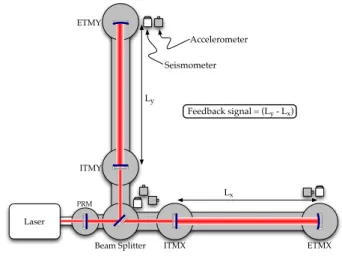
Instead of a single cavity, in this case we explored the subtraction of seismic noise from the differential arm length feedback signal (which is an accurate measure of the low frequency ground noise). The sensors are placed close to the ends of the interferometer arms and at the beamsplitter as shown in Figure 4.
Beam Splitter ITMX ETMX ITMY ETMY PRM Ly Lx Feedbacksignal= (Ly - Lx) Laser Accelerometer Seismometer
FIG. 4. Schematic layout of seismometers relative to interfer-ometer mirrors.
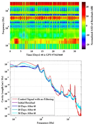
4 Figure 5 shows the resulting subtraction efficacy for
a static filter. The variation in the 0.1-0.3 Hz band comes from variation in the ambient level of the dou-ble frequency microseismic peak17. The structure in the
1-15 Hz band is the usual increase in anthropogenic noise during the workday.
Even though some excess noise is added in the dips around 3-5 Hz and 7 Hz, the filter reduces the main con-tributors to the RMS of the control signal, and the re-duction is remarkably stable over the 30 day timespan. This static filter does inject an unacceptable amount of noise above 20 Hz, which we will elimiate in the future by using more aggresive pre-weighting to disallow such noise amplification before calculating the Wiener filter.
Figure 6 shows the subtraction if we use an acausal filter, retraining it every 10 minutes, for the same 30 day data set. This filter performs much better than the static version. While we cannot apply an acausal filter in re-altime, we can utilize causal adaptive filters to achieve nearly the same effect as long as the seismic environment does not change appreciably on time scales less than 10 minutes.
Residuals for both Figures 5 and 6 were calculated us-ing 46 second long Wiener filters of 3000 taps at a sample rate of 64 Hz.
V. ONLINE ADAPTIVE FILTERING AT THE 40M INTERFEROMETER
In case the transfer functions between the sensors and the target are changing with time, it would be useful to use a filter whose coefficients change with time. Such an adaptive filter could also take into account changes in the ’actuator’. The most simple and common imple-mentation of an adaptive filter is the Least Mean Squares (LMS) algorithm18.
The Online Adaptive Filtering (OAF) algorithm im-plemented at the 40m Lab is the Filtered-x Least Mean Squared (FxLMS) algorithm19. It is based primarily on
the canonical LMS algorithm; a steepest descent opti-mization of a defined error function. Just as in the static Wiener filtering in Section II, we minimize the RMS of the difference between the filtered output and the orig-inal feedback signal. The LMS algorithm described in Equation 4 takes ’steps’ in the direction of the steepest gradient until it arrives at a local minima.
w(n + 1) = w(n) × [1 − τ ] + µ × e(n) × x(n) (4) Here the next iteration’s FIR coefficients depend on the the current coefficients (w), the current witness sig-nal (x), the current error sigsig-nal (difference between the target and filtered signal, e), and the adaptation rate (µ). One of the largest challenges with the adaptive filtering algorithm is that the success of the algorithm is fairly sensitive to the choice of µ. To improve stability against
FIG. 5. (Color online) Result of offline simulated seismic Wiener filtering on the 4km LIGO Hanford interferometer. (a) Traces are amplitude spectra normalized to the unfiltered control signal (red trace in b), which is at a time during the filter’s training. Filter was trained on 6 hours of data, then applied in 10 minute segments. Vertical stripes indicate times when the interferometer was not operational. Seismic sub-traction is fairly constant on a one month time scale, although it is not particularly effective for times when seismic noise is significantly different from the training time (b) Selected in-dividual spectra from a above. Dotted red trace is before subtraction, purple trace is initial residual and progressively lighter blues are 10, 20 and 30 days after the filter was trained.
transients, we modify the usual FxLMS algorithm to in-clude a decay constant τ .
The FxLMS algorithm acknowledges that there exist phase delays in the path of the target signal which can-not be approximated by the LMS method alone20. To
account for these phase delays, we filter the incoming witness signals with filters identical to those in the tar-get signal path. Once we have matched the delays in the two different paths, we implement the regular LMS op-timization to find the coefficients we will use in our FIR filter. The FxLMS algorithm used is sketched in Figure 7. We apply the OAF system to the same triangular cav-ity as in Section III. Once again, we use the cavcav-ity length feedback signal as our targeted signal to minimize, and a similar layout of independent witness sensors as shown
FIG. 6. (Color online) Result of offline simulated seismic Wiener filtering on the 4km LIGO Hanford interferometer, using an acausal filter on the same 30 day data set. (a) Traces are amplitude spectra normalized to the unfiltered control sig-nal (red trace in b). A filter is trained on, and then applied to, 10 minute segments of data. Seismic noise is more effectively suppressed using this constantly updated filter, implying that the transfer function is changing on a relatively short time scale, and that it is advantageous to update the filter more often than once per month. (b) Selected individual spectra from a above. Dotted red trace is before subtraction, purple trace is initial residual and progressively lighter blues are 10, 20 and 30 days after beginning.
Adaptation
FIR Filter
Matching Filter (Plant Estimate) Witness Sensor Cavity Length Feedback Signal Plant (Mirror, Cavity, etc.)FIG. 7. Block diagram of the FxLMS algorithm used.
in Figure 1. Unlike Sections III and IV which were sim-ulations using previously collected data, here we are ac-tuating on the cavity in realtime. Figure 8 shows results using a 125 second long, 2000 tap filter with µ = 0.01 and τ = 10−6 at a 16 Hz sample rate. The on /off traces
in the adaptive case are similar to estimates made in the static Wiener filtering case (Figure 2). Given enough time to adapt, the OAF converges towards the optimal filter, but, so far, not completely. Since the adaptive system was tested using one G¨uralp seismometer9 and
one Ranger SS-1 seismometer21, the subtraction is not as pronounced as if we had used 2 G¨uralps, or other more sensitive broadband seismometers. In the next iteration of this setup, we will explore the variation in the cancel-lation performance as a function of sensor placement.
Frequency (Hz) -1 10 1 10 ) 1/2 Cavity Length (m/Hz -11 10 -10 10 -9 10 -8 10 -7 10 Control Signal: FF ON Control Signal: FF OFF
FIG. 8. (Color online) Online Adaptive Filter performance: the spectral density of the cavity length fluctuations are shown with the feed-forward on (lower blue trace) and off (upper red trace).
VI. CONCLUSIONS
We have demonstrated the use of Wiener filter based feed-forward seismic noise reduction on a suspended in-terferometer. We have also implemented a stable, adtive feed-forward system which has a performance ap-proaching that of the optimal Wiener estimate. These techniques can be simply implemented in any general laboratory requiring vibration isolation using relatively low cost accelerometers and commodity computers and DSP software (e.g. Labview). These ’optimal’ feed-forward schemes operate without having to know a priori the transfer function between the disturbance and the primary experiment; they can easily be reconfigured to adapt to new experimental setups. Similar Wiener filter and LMS based techniques have been utilized in other experiments, both offline and online, for example isolat-ing 2-mirror Fabry-Perot cavities from ground motion22,
reducing acoustic noise in oceanography settings23and in signal processing to decorrelate degenerate witness chan-nels24.
In the near future, we will work to use this scheme to reduce the noise in multiple degrees of freedom of the full interferometer. It is clear that this technique can also be
6 applied to remove other sources of environmental noise
(e.g. acoustic, magnetic, electronic, etc.). For each noise source in the gravitational wave band, we will inject soft-ware gravitational wave signals into the data stream and confirm that they are not distorted. There will certainly be new challenges associated with each type of noise, but this seems promising as a method which can be employed to reduce the influence of environmental noise in a wide variety of experimental setups.
VII. ACKNOWLEDGEMENTS
We gratefully acknowledge illuminating discussions with Joe Giaime, Alan Weinstein, Rob Ward, and Jan Harms. We also thank the National Science Foundation for support under grant PHY-0555406. J. Driggers also acknowledges the support of an NSF Graduate Research Fellowship. K. Pepper acknowledges the support of the LIGO NSF REU program. LIGO was constructed by the California Institute of Technology and Massachusetts In-stitute of Technology with funding from the National Sci-ence Foundation and operates under cooperative agree-ment PHY-0107417. This article has LIGO Docuagree-ment Number P0900071.
1B. P. Abbott, R. Abbott, R. Adhikari, P. Ajith, B. Allen, G.
Allen, R. S. Amin, S. B. Anderson, W. G. Anderson, M. A. Arain, M. Araya, H. Armandula, P. Armor, Y. Aso, S. Aston, P. Auf-muth, C. Aulbert, S. Babak, P. Baker, S. Ballmer, C. Barker, D. Barker, B. Barr, P. Barriga, L. Barsotti, M. A. Barton, I. Bartos, R. Bassiri, M. Bastarrika, B. Behnke, M. Benacquista, J. Betzwieser, P. T. Beyersdorf, I. A. Bilenko, G. Billingsley, R. Biswas, E. Black, J. K. Blackburn, L. Blackburn, D. Blair, B. Bland, T. P. Bodiya, L. Bogue, R. Bork, V. Boschi, S. Bose, P. R. Brady, V. B. Braginsky, J. E. Brau, D. O. Bridges, M. Brinkmann, A. F. Brooks, D. A. Brown, A. Brummit, G. Brunet, A. Bullington, A. Buonanno, O. Burmeister, R. L. Byer, L. Cado-nati, J. B. Camp, J. Cannizzo, K. C. Cannon, J. Cao, L. Carde-nas, S. Caride, G. Castaldi, S. Caudill, M. Cavaglia, C. Cepeda, T. Chalermsongsak, E. Chalkley, P. Charlton, S. Chatterji, S. Chelkowski, Y. Chen, N. Christensen, C. T. Y. Chung, D. Clark, J. Clark, J. H. Clayton, T. Cokelaer, C. N. Colacino, R. Conte, D. Cook, T. R. C. Corbitt, N. Cornish, D. Coward, D. C. Coyne, J. D. E. Creighton, T. D. Creighton, A. M. Cruise, R. M. Culter, A. Cumming, L. Cunningham, S. L. Danilishin, K. Danzmann, B. Daudert, G. Davies, E. J. Daw, D. DeBra, J. Degallaix, V. Dergachev, S. Desai, R. DeSalvo, S. Dhurandhar, M. Diaz, A. Di-etz, F. Donovan, K. L. Dooley, E. E. Doomes, R. W. P. Drever, J. Dueck, I. Duke, J-C. Dumas, J. G. Dwyer, C. Echols, M. Edgar, A. Effler, P. Ehrens, E. Espinoza, T. Etzel, M. Evans, T. Evans, S. Fairhurst, Y. Faltas, Y. Fan, D. Fazi, H. Fehrmenn, L. S. Finn, K. Flasch, S. Foley, C. Forrest, N. Fotopoulos, A. Franzen, M. Frede, M. Frei, Z. Frei, A. Freise, R. Frey, T. Fricke, P. Fritschel, V. V. Frolov, M. Fyffe, V. Galdi, J. A. Garofoli, I. Gholami, J. A. Giaime, S. Giampanis, K. D. Giardina, K. Goda, E. Goetz, L. M. Goggin, G. Gonzalez, M. L. Gorodetsky, S. Gossler, R. Gouaty, A. Grant, S. Gras, C. Gray, M. Gray, R. J. S. Greenhalgh, A. M. Gretarsson, F. Grimaldi, R. Grosso, H. Grote, S. Grunewald, M. Guenther, E. K. Gustafson, R. Gustafson, B. Hage, J. M. Hallam, D. Hammer, G. D. Hammond, C. Hanna, J. Hanson, J. Harms, G. M. Harry, I. W. Harry, E. D. Harstad, K. Haughian, K. Hayama, J. Heefner, I. S. Heng, A. Heptonstall, M. Hewitson, S. Hild, E. Hirose, D. Hoak, K. A. Hodge, K. Holt, D. J. Hosken, J. Hough, D. Hoyland, B. Hughey, S. H. Huttner, D. R. Ingram, T. Isogai,
M. Ito, A. Ivanov, B. Johnson, W. W. Johnson, D. I. Jones, G. Jones, R. Jones, L. Ju, P. Kalmus, V. Kalogera, S. Kandhasamy, J. Kanner, D. Kasprzyk, E. Katsavounidis, K. Kawabe, S. Kawa-mura, F. Kawazoe, W. Kells, D. G. Keppel, A. Khalaidovski, F. Y. Khalili, R. Khan, E. Khazanov, P. King, J. S. Kissel, S. Klimenko, K. Kokeyama, V. Kondrashov, R. Kopparapu, S. Ko-randa, D. Kozak, B. Krishnan, R. Kumar, P. Kwee, P. K. Lam, M. Landry, B. Lantz, A. Lazzarini, H. Lei, M. Lei, N. Leindecker, I. Leonor, C. Li, H. Lin, P. E. Lindquist, T. B. Littenberg, N. A. Lockerbie, D. Lodhia, M. Longo, M. Lormand, P. Lu, M. Lu-binski, A. Lucianetti, H. Lueck, B. Machenschalk, M. MacInnis, M. Mageswaran, K. Mailand, I. Mandel, V. Mandic, S. Marka, Z. Marka, A. Markosyan, J. Markowitz, E. Maros, I. W. Martin, R. M. Martin, J. N. Marx, K. Mason, F. Matichard, L. Matone, R. A. Matzner, N. Mavalvala, R. McCarthy, D. E. McClelland, S. C. McGuire, M. McHugh, G. McIntyre, D. J. A. McKechan, K. McKenzie, M. Mehmet, A. Melatos, A. C. Melissinos, D. F. Menendez, G. Mendell, R. A. Mercer, S. Meshkov, C. Messenger, M. S. Meyer, J. Miller, J. Minelli, Y. Mino, V. P. Mitrofanov, G. Mitselmakher, R. Mittleman, O. Miyakawa, B. Moe, S. D. Mo-hanty, S. R. P. Mohapatra, G. Moreno, T. Morioka, K. Mors, K. Mossavi, C. MowLowry, G. Mueller, H. Mueller-Ebhardt, D. Muhammad, S. Mukherjee, H. Mukhopadhyay, A. Mullavey, J. Munch, P. G. Murray, E. Myers, J. Myers, T. Nash, J. Nelson, G. Newton, A. Nishizawa, K. Numata, J. O’Dell, B. O’Reilly, R. O’Shaughnessy, E. Ochsner, G. H. Ogin, D. J. Ottaway, R. S. Ot-tens, H. Overmier, B. J. Owen, Y. Pan, C. Pankow, M. A. Papa, V. Parameshwaraiah, P. Patel, M. Pedraza, S. Penn, A. Perraca, V. Pierro, I. M. Pinto, M. Pitkin, H. J. Pletsch, M. V. Plissi, F. Postiglione, M. Principe, R. Prix, L. Prokhorov, O. Punken, V. Quetschke, F. J. Raab, D. S. Rabeling, H. Radkins, P. Raffai, Z. Raics, N. Rainer, M. Rakhmanov, V. Raymond, C. M. Reed, T. Reed, H. Rehbein, S. Reid, D. H. Reitze, R. Riesen, K. Riles, B. Rivera, P. Roberts, N. A. Robertson, C. Robinson, E. L. Robin-son, S. Roddy, C. Roever, J. Rollins, J. D. Romano, J. H. Romie, S. Rowan, A. Ruediger, P. Russell, K. Ryan, S. Sakata, L. San-cho de la Jordana, V. Sandberg, V. Sannibale, L. Santamaria, S. Saraf, P. Sarin, B. S. Sathyaprakash, S. Sato, M. Satterthwaite, P. R. Saulson, R. Savage, P. Savov, M. Scanlan, R. Schilling, R. Schnabel, R. Schofield, B. Schulz, B. F. Schutz, P. Schwinberg, J. Scott, S. M. Scott, A. C. Searle, B. Sears, F. Seifert, D. Sellers, A. S. Sengupta, A. Sergeev, B. Shapiro, P. Shawhan, D. H. Shoe-maker, A. Sibley, X. Siemens, D. Sigg, S. Sinha, A. M. Sintes, B. J. J. Slagmolen, J. Slutsky, J. R. Smith, M. R. Smith, N. D. Smith, K. Somiya, B. Sorazu, A. Stein, L. C. Stein, S. Steplewski, A. Stochino, R. Stone, K. A. Strain, S. Strigin, A. Stroeer, A. L. Stuver, T. Z. Summerscales, K-X. Sun, M. Sung, P. J. Sutton, G. P. Szokoly, D. Talukder, L. Tang, D. B. Tanner, S. P. Tarabrin, J. R. Taylor, R. Taylor, J. Thacker, K. A. Thorne, A. Thuering, K. V. Tokmakov, C. Torres, C. Torrie, G. Traylor, M. Trias, D. Ugolini, J. Ulmen, K. Urbanek, H. Vahlbruch, M. Vallisneri, C. Van Den Broeck, M. V. van der Sluys, A. A. van Veggel, S. Vass, R. Vaulin, A. Vecchio, J. Veitch, P. Veitch, C. Veltkamp, A. Vil-lar, C. Vorvick, S. P. Vyachanin, S. J. Waldman, L. Wallace, R. L. Ward, A. Weidner, M. Weinert, A. J. Weinstein, R. Weiss, L. Wen, S. Wen, K. Wette, J. T. Whelan, S. E. Whitcomb, B. F. Whiting, C. Wilkinson, P. A. Willems, H. R. Williams, L. Williams, B. Willke, I. Wilmut, L. Winkelmann, W. Winkler, C. C. Wipf, A. G. Wiseman, G. Woan, R. Wooley, J. Worden, W. Wu, I. Yakushin, H. Yamamoto, Z. Yan, S. Yoshida, M. Zanolin, J. Zhang, L. Zhang, C. Zhao, N. Zotov, M. E. Zucker, H. zur Muehlen, J. Zweizig, Rep. Prog. Phys., 72, 076901 (2009).
2P. R. Saulson, Phys. Rev. D, 30, 732 (1984).
3S. A. Hughes and K. S. Thorne, Phys. Rev. D, 58, 122002 (1998). 4M. Beccaria, M. Bernardini, S. Braccini, C. Bradaschia, A. Bozzi,
C. Casciano, G. Cella, A. Ciampa, E. Cuoco, G. Curci, E. D’Ambrosio, V. Dattilo, G. De Carolis, R. De Salvo A. Di Vir-gilio, A. Delapierre, D. Enard, A. Errico, G. Feng, I. Ferrante, F. Fidecaro, F. Frasconi, A. Gaddi, A. Gennai, G. Gennaro, A. Giazotto, P. La Penna, G. Losurdo, M. Maggiore, S. Mancini, F.
Palla, H. B. Pan, F. Paoletti, A. Pasqualetti, R. Passaquieti, D. Passuillo, R. Poggiani, P. Popolizio, F. Raffaelli, S. Rapisarda, A. Vicere, Z. Zhang, Class. Quantum Grav., 15, 3339 (1998).
5S. Haykin, Adaptive Filter Theory, 4th ed. (Prentice Hall, 2002). 6J. Durbin, Rev. Inst. Int. Stat., 28, 233 (1960).
7Y. Huang, J. Benesty, and J. Chen, Acoustic MIMO Signal
Processing (Springer, Signals and Communication Technology, 2006).
8R. Ward, Length sensing and control of a prototype advanced
interferometric gravitational wave detector, Ph.D. thesis, Cali-fornia Institute of Technology (2010).
9G¨uralp Systems Ltd., “CMG-40T: Triaxial broadband
seismome-ter,” (2009).
10Wilcoxon Research, “731a ultra-quiet, ultra low frequency
seis-mic accelerometer,” (2009).
11J. A. Giaime, Studies of Laser Interferometer Design and a
Vi-bration Isolation System for Interferometric Gravitational Wave Detectors, Ph.D. thesis, Massachusetts Institute of Technology (1995).
12J. A. Giaime, P. Saha, D. Shoemaker, and L. Sievers, Rev. Sci.
Instrum., 67, 208 (1996).
13MathWorks, “MATLAB 2010,”.
14N. A. Robertson, B. Abbott, R. Abbott, R. Adhikari, G. Allen,
H. Armandula, S. Aston, A. Baglino, M. Barton, B. Bland, R. Bork, J. Bogenstahl, G. Cagnoli, C. Campbell, C. A. Cantley, K. Carter, D. Cook, D. Coyne, D. Crooks, E. Daw, D. DbBra, E. El-liffe, J. Faludi, P. Fritschel, A. Ganguli, J. Giaime, S. Gossler, A. Grant, J. Greenhalgh, M. Hammond, J. Hanson, C. Hardham,
G. Harry, A. Heptonstall, J. Heefner, J. Hough, D. Hoyland, W. Hua, L. Jones, R. Jones, J. Kern, J. LaCour, B. Lantz, K. Lilienkamp, N. Lockerbie, H. Lueck, M. MacInnis, K. Mailand, K. Mason, R. Mittleman, S. Nayfeh, J. Nochol, D. J. Ottaway, H. Overmier, M. Perreur-Lloyd, J. Phinney, M. Plissi, W. Rankin, D. Robertson, J. Romie, S. Rowan, R. Scheffler, D. H. Shoe-maker, P. Sarin, P. Sneddon, C. Speake, O. Spjeld, G. Stapfer, K. A. Strain, C. Torrie, G. Traylor, J. van Niekerk, A. Vecchio, S. Wen, P. Willems, I. Wilmut, H. Ward, M. Zucker, L. Zuo, Proc. SPIE, 5500, 81 (2004).
15S. Wen, Improved Seismic Isolation for The Laser Interferometer
Gravitational Wave Observatory with Hydraulic External Preiso-lator System, Ph.D. thesis, Louisiana State University (2009).
16R. deRosa, J. Driggers, D. Atkinson, H. Miao, V. Frolov,
M. Landry, and R. Adhikari, “Global feed-forward vibration isolation in a km scale interferometer,” (in preparation).
17R. A. Haubrich and K. McCamy, Rev. Geophys., 7, 539 (1969). 18A. H. Sayed, Fundamentals of Adaptive Filtering (IEEE Press,
Wiley-Interscience, University of California, Los Angeles, 2003).
19B. Widrow and S. D. Stearns, Adaptive Signal Processing
(Pren-tice Hall, 1985).
20National Instruments, “Filtered-x LMS algorithms,” (2009). 21Kinemetrics, “SS-1 Ranger Seismometer,” (2008).
22M. J. Thorpe, D. R. Leibrandt, T. M. Fortier, and T. Rosenband,
Opt. Express, 18, 18744 (2010).
23C. W. Therrien, K. L. Frack Jr, and N. R. Fontes (IEEE Intl.
Conf. on Acoustics, Speech and Signal Processing, 1997) pp. 543– 546.