Adaptive Functional Magnetic Resonance Imaging
bySeung-Schik Yoo
B.S., Biomedical Engineering, The Johns Hopkins University, 1994 M. of Business Administration, University of Massachusetts, Boston, 1999
Submitted to the Department of Nuclear Engineering and Harvard-M.I.T. Division of Health Science and Technology in Partial Fulfillment of the Requirements for the Degree of
Doctor of Philosophy in the field of Radiological Science at the
MASSACHUSETTS INSTITUTE OF TECHNOLOGY February, 2000
@ 2000 Massachusetts Institute of Technology. All rights reserved
OF TECHNOP.
LIBRARIES
Scine
'I
Author... ...
...
...
...
...
...
...
...
...
...
...
...
...
...
...
...
...
...
...
...
...
...
...-.
.
.. ... -.. ... ... ... .'r. .-Department of Nuclear Engin /ring Harvard-M.I.T. Division of Health Science and Technology January, 25, 2000
Certified by ... ... ... ... ... ... ... ... ... ... . .. ... ... .. .. ... .. . ... ... ... ... ... . .. .... .. , ... ... Lawrence P. Panych Assistant Professor of Radiology, Harvard Medical School Thesis Supervisor
Certified by ... ... ... ... ... ... ... ... ... ... ... ... ...
ory Associate Professor of Nuclear Engineering Thesis Reader
A ccepted by... ... ... ... ... ... ... ... ... ... ... ... ... ... ... .... ... ... ... ... ... ... ... ... ... ... ... ... ... ... ... ... Sow-Hsin Chen Professor of Nuclear Engineering Chairman, Department Committee on Graduate Students
Adaptive Functional Magnetic Resonance Imaging
by
Seung-Schik Yoo
Submitted to the Department of Nuclear Engineering and Harvard-M.I.T. Division of Health Science and Technology
on January 27, 2000 in partial fulfillment of the requirements for the degree of
Doctor of Philosophy in the field of Radiological Science
Abstract
Functional MRI (fMRI) detects the signal associated with neuronal activation, and has been widely used to map brain functions. Locations of neuronal activation are localized and distributed throughout the brain, however, conventional encoding methods based on k-space acquisition have limited spatial selectivity. To improve it, we propose an adaptive fMRI method using non-Fourier, spatially selective RF encoding. This method follows a strategy of zooming into the locations of activation by progressively eliminating the regions that do not show any apparent activation. In this thesis, the conceptual design and implementation of adaptive fMRI are pursued under the hypothesis that the method may provide a more efficient means to localize functional activities with increased spatial or temporal resolution.
The difference between functional detection and mapping is defined, and the multi-resolution approach for functional detection is examined using theoretical models simulating variations in both in-plane and through-plane resolution. We justify the multi-resoltion approach experimentally using BOLD CNR as a quantitative measure and compare results to those obtained using theoretical models. We conclude that there is an optimal spatial resolution to obtain maximum detection; when the resolution matches the size of the functional activation.
We demonstrated on a conventional 1.5-Tesla system that RF encoding provides a simple means for monitoring irregularly distributed slices throughout the brain without encoding the whole volume. We also show the potential for increased signal-to-noise ratio with Hadamard encoding as well as reduction of the in-flow effect with unique design of excitation pulses.
RF encoding was further applied in the implementation of real-time adaptive fMRI method, where we can zoom into the user-defined regions interactively. In order to do so, real-time pulse prescription and data processing capabilities were combined with RF encoding. Our specific implementation consisted of five scan stages tailored to identify the volume of interest, and to increase temporal resolution (from 7.2 to 3.2 seconds) and spatial resolution (from 10 mm to 2.5-mm slice thickness). We successfully demonstrated the principle of the multi-resolution adaptive fMRI method in volunteers performing simple sensorimotor paradigms for simultaneous activation of primary motor as well as cerebellar areas.
Thesis Supervisor: Lawrence P. Panych
Table of Contents
Acknowledgem ents... ... ... .. ... ... .. ... ... ... ... ... ... ... . ... ... ... ... ... ... ...
7
Chapter 1. Introduction to Adaptive fMRI and Magnetic Resonance Imaging
1.1 Introduction ... ... ... ... ...
.
.. ... .
.
.
..
...
... ...
. ..
... ... ... ... ..
8
1.2 Magnetic Resonance Imaging
1.2.1
Physics of N M R: The Signal Source... ... ... ... ... ... ... ... ... ..
..
.. ... ... ... ... ... .
12
1.2.2
MR Signal; Excitation, Precession, and Relaxation... ... ... ... ... ... ... ... ... ... ...
13
1.2.3
Imaging and Encoding... ... .. ... ...
...
... ... ..
....
... ... ... ... .
17
1.2.4
M R Signal and Contrast... ... ... ... ... ... ... .. ... ... ... ... ... ... ... ... ... .... ... ...
24
Chapter
2.
Fundamentals of Functional MRI
2.1 Introduction... ... ... ... ... ... ... ... ... ...
....
... ... . ... .. .... ... ... ... ... ... ... ... ... ...
27
2.2 Contrast in fMiRI
2.2.1
Physiological Basics in Neuronal Activation... ... ... ... .. ... ... ... ... ... .... .
28
2.2.2
Contrast Mechanisms in Functional MRI... ... ... . ... ... ... ... ... ...
... ... ... .
29
2.2.3
BO LD Contrast... ... ... ... ... ... ... ... ... ...
... ... ...
...
... ...
... ... ... ... ..
30
2.3 Overview of fMRI Experiment
2.3.1
Experimental Design and Procedure... ... ... ... ... ... ... ... ...
... ... ... ... ...
33
2.3.2
Data Acquisition M ethods... ... ... ... ... ... ...
... ... ... ... ... ... ... .. ... ... ...
35
2.3.3
Event-Related Design... ... .. ... ...
...
... ... ..
....
... .... ... ... ... ..
37
Chapter 3. Spatially-selective RF Encoding
3.1 Introduction
3.1.1
RF Selective Excitation... ... .. ... ...
...
... ... ..
....
... ... ... ... ... .... .
38
3.1.2
Matrix Representation of RF encoding... .
... ...
...
.. ...
... ... ... ...
40
3.2 Point-Spread Function of RF encoding
3.2.1
Cross-talk in RF Encoding ... ... ... ... ... ... ...
....
... ... ... ... .
43
3.3 RF Encoding for fMIRI
3.3.1
Matrix Representation... ... .. ... ...
...
... ... ..
....
... ... ... ... ... .
46
3.3.2
G eneral SN R Analysis... ... ... ... ... ... ... .. ... ... ... ... ... ... ... ... ... . ... ... ... .
48
3.3.3
SNR of Hadamard and Multi-Slice Encoding ...
... ... ... ... ... ... .
50
3.4 Sum m ary... ... ... ... ... ... ...
. .. ... ... ...
... ... ... . .. ... ... ... ... ... ... ...
52
Chapter 4. Multi-resolution Detection of Functional Activation:
Theoretical Examination
4.1 Introduction... ... ... ...
... ... ... ... ... ... ... ... ... ..
... .... . .. ... ..
53
4.2 BOLD Signal Detection...
... ... ... ... ... ... ...
... ... ... ... ... ...
... ... ... ... ... .. ..
54
4.3 Temporal Resolution and BOLD CNR... ...
... .
...
..
... ... ... .... ..
55
4.4 In-plane Resolution and BOLD CNR
4.4.1
Tw o-voxel M odel... ... ... ... ... ... ... ... ... ... ... ... ... ... ...
.
.. ... ... ... ... ... ... .
57
4.4.2
In-plane Resolution and BOLD CNR ... ... ... ... ... ... ... ... ... ... ... ... ... .
59
4.5 Slice Thickness, Size of Activation and BOLD CNR
4.5.1
Two-slice M odel... ... ... ... ... ... ... ... ... ...
.
.
.
.... ... ... ... ... .. ...
... .. ..
63
4.5.2
Slice Thickness and BOLD CNR. ... ... ... ... ... ...
... ... ...
... ... ... ... ... ... .
65
4.6 Physiological Noise and CNR... ... ... ... ... ... ... ... ... ..
.
..
.... . ...
... ... ... ... .... .
68
4.7 Summary ... ... ... ... ... ...
...
...
...
... ... ... ... ... ... ... ... ... ... ... ... ... ... .
70
Chapter 5. Multi-resolution Detection of Functional Activation: Experimental Data
5.1 Introduction... ... ... ... ... ...
...
... ... ...
...
... .. . ...
...
...
... ... ...
72
5.2 Materials and Methods
5.2.1
D ata Processing... ... ... ... ... ... ... ... ... ... ... ... ...
... ... ...
... ... ... ... ...
73
5.2.2
Variation of In-plane Resolution... ... ... ... ... ... ...
... ...
... ... ... ..
74
5.2.3
Variation of Slice Thickness... ... ... ... ... ... .... ... ... ... ... . ... ... .... .
74
5.2.4
Simulation of Multi-resolution Detection ... ... ... ... ... ... ... ... ... ... ... ...
75
5.3 Results
5.3.1
Variation of In-plane Resolution ... ... ...
... ... ... ... ...
.. .. .. ... ... ... .
76
5.3.2
Variation in Slice Thickness.. ... ... ...
. . ....
...
... ... ... . ... ....
78
5.3.3
Simulation of Multi-resolution Detection ... ...
... ... ... ... ... ... ...
81
5.3.4
Noise Level Dependency on Slice Thickness... ... ... ... ... ... ... ... ...
.. ..
83
5.4 Sum m ary... ... ... ... ... ... ... ... ... ... ... ...
...
..
... ...
... ...
... ... ... .. ...
... ...
. 84
Chapter 6. Functional
MRI
using Spatially-selective RF encoding
6.1 Introduction... ... ... ... ... ... ... ....
... .
.. ... ...
...
... .. . ...
...
... ... ... ...
86
6.2 Materials and Methods
6.2.1
Multi-slice Imaging... ... ... ... ... ... ... ...
...
... ... ... ... ... ...
... ... ...
88
6.2.2
Hadamard Encoding... ... ... ... ... ... ... ... ... ..
.
... ... ... ...
... ... ... ... ... ... .
89
6.2.3
Task Paradigms and Data Analysis ... ... ... ...
...
....
...
... ... ... ...
90
6.3 Results
6.3.1
Activation M ap... ... ... ... ... ...
... ... ... ... ...
... ...
... ... ... .
91
6.3.2
ROI Analysis for In-flow Reduction... ... ... ... ... ... ... ... ..
....
... ... ... ... ... ..
92
Chapter 7. Real-time Adaptive Functional MRI
7.1 Introduction ... ... ... ... ... ... ... ... ... ... ... ... ... ... ... ... ... ... ... ... ... ... ... ... ... ... ... ... .
98
7.2 Materials and Methods
7.2.1
Subjects and Imaging Acquisition... ... ... ... ... ... ... ... ..
.
... ... ... ... ... ... ... ..
101
7.2.2
Hardware and Software Configuration for Real-time Adaptive System... ... ..
103
7.3 Results
7.3.1
Real-time Adaptive Functional MRI...
... ... ... ... ... ... ... ... ... ... .. ..
105
7.3.2
Quantitative Evaluation at Multiple-Resolutions... ... ... ... .. ... ... ... ... ... ...
108
7.4 Sum m ary... ... ... ... ... ... ... ... ... ... ... ... ... ... ...
.
.. ... ... ... . ...
... ... . .. ...
... ... ... .
110
Chapter 8. Discussions and Conclusions
8.1 Introduction ... ... ... ... ... ... ...
... .
.. ..
..
... ... ... .. . .. ... ... .. .
111
8.2 Multi-resolution Detection of Activation... ... ... ... ... ... ... ... ... ... ...
... ... ...
112
8.3 RF Encoding for Functional MRI... ... ... ... ... ... ... ... ... ... ... ... ...
... .
116
8.4 Real-time Adaptive fMIRI... ... ... ... ...
...
... ... ...
... ...
... ... ...
...
... ... ... .. ..
119
8.5 Applications of Adaptive Approach... ... ... ... ... ... ... ... ... ... ..
.
...
... ... ... .. ... ... ... .
120
8.6 Future Studies... ... ... ... ... ... ... ... ... ... ... ... ... ... ... ... ... ... ... ... ... ... ... ... ... ... ... ..
121
8.7 Conclusions ... ... ... ... ... ... ...
... ... ... ... ... ... ... ... ... ... ... ... ... ... ... ... .
123
L ist of Sym bols... ... ... ... ... ... ... ... ... .. . ... ... ... ... ...
. ... ... ... ... ... ... ... ...
126
L
ist
o
f
F
ig
es... ... ... ... ... ... ... ... ... ... ... ... ... ... ... ... ... ... ... ... ... ...
128
L ist of
T
ables ... ... ... ... ... ... ... ... ... ... ... ... ... ... ... ... ... ... ... . ..
... ... . .. ...
131
Acknowledgements
I would like to take this opportunity to acknowledge my thesis supervisor, Professor Lawrence P. Panych, for his guidance and mentorship during my graduate study. I feel I am very lucky to have him as my advisor. I owe so much to him. His instruction helped me to become an endeavoring research scientist. I also thank his wife, Dr. Chandlee Dickey for her kind words and smile.
I extend my thanks to Dr. Guttmann. He has been a good friend, a mentor, and a keen critic on my thesis work. Without him, submitting this thesis would have been quite a difficult task. I would also like to thank Professor David Cory. He taught me about radiological sciences and was also a persistent supporter of my thesis and work. I really appreciate his help and advice. Professor Rosen, who paved the way for functional MRI, helped me to set my vision on functional MRI as well as advised me through HST program. Dr. Wible, an inspiring neuroscientist, helped to introduce me to the world of neuroscience. I was very fortunate to have them in the thesis committee.
Professor Jolesz always was a good supporter of my work, and I thank him for his supportive words. I also would like to thank Drs. Rivkin, Weiler, Mulkern, and Waber at Children's Hospital for their support. Dr. Rivkin especially allowed me to concentrate on writing my thesis at times when I was supposed to dedicate more time to his research. I should not fail to acknowledge Drs. Tung and Horowitz at Johns Hopkins Medical School, and Dr. Muller at FDA, who helped me to initiate my career in the field of medical research.
I acknowledge my colleagues, Drs. Saiviroonporn, Zhao, Cavanaugh, Kacher, Kyriakos, Zengingonul and Venkatesh at Brigham and Women's Hospital for their friendship and support. My graduate life would have been much less fun without them. In particular, Dr. Bernard, the director of the MIT nuclear reactor, pampered and guided me through the qualifying exam. My colleagues at MIT and HST, Drs. Justo, Tang, Ju, Liu, Sha and Seto are great scientists and fun-friends to be with. They were always supportive even though I was rarely on campus. Professor Yip, Zhou and Chen were always available for help and guidance. Ms. Gwinn, Egan at MIT and administrative staffs at Brigham, Ms.Valk, Roth, Holub and Kelly, were eager to help me with administrative problems. I will remember their help and appreciate it.
I would also like to dedicate this thesis to my late sister, Sung-Min, who, I believe, is watching over me. I also thank my sister, Sung-Hee, who motivated me to come to U.S. about 9 years ago, for her strong support. I owe everything else to my parents, Hyon-Joon Yoo and Yoo-Wan Sung. They nurtured me and supported me incessantly in all aspects of my life. I dare endeavor to be the greatest parents as they are. There are no words to describe how much I am thankful for their support. Last, but not least, I dedicate this thesis to my dearest wife, Seh-Eun, my daughter Jung-Yeon and my family-in-laws. Seh-Eun endured nine long months as a wife of a graduate student and as a mother-to-be while I had to concentrate on my thesis and research. Seh-Eun has helped and encouraged me to stay on course. I also thank all her family for their strong support.
Chapter 1
Introduction to Adaptive fMRI and
Magnetic Resonance Imaging
1.1 Introduction
Functional magnetic resonance imaging (fMRI) was developed in the early 1990s capitalizing upon the ability to detect local changes in cerebral blood volume (CBV), cerebral blood flow (CBF) and oxygenation level during neuronal activation ([1]-[7]). It has since achieved a prominent place in methods for mapping brain function. Functional MRI enables non-invasive visualization of brain function, without resorting on the use of radioactive or exogenous contrast agents. With good temporal and spatial resolution, functional MRI has been used in numerous neuro-scientific studies including somatotopic cortical mapping ([8]-[10]) and the investigation of high-order cognitive processes such as working memory and decision making ([11]-[15]). Functional MRI has also had a direct impact on clinical applications. These include functional mapping of cortical areas for the planning of neuro-surgery ([16]-[19]) as well as elucidating the neural difference of people with psychiatric /cognitive disorders such as schizophrenia and learning disability [20,21].
The most common and widely used method for eliciting functional signal is based on the detection of the blood oxygenation level dependent (BOLD) variation during neuronal activation using imaging sequences that are sensitive to the local changes in magnetic susceptibility. BOLD contrast in cortical tissue is small, typically on the order of between 1% and 6% at 1.5 Tesla [22]. In a typical fMRI experiment, multiple sets of images are acquired over the course of several control and stimulation periods and the small BOLD change due to activation is detected using statistical methods ([23]-[25]). In general, acquiring the data from the whole brain is important because the area of brain activation is not always known a priori, nor is it necessarily confined to a single slice of the imaging volume. In particular, high-order functional tasks involving multiple locations throughout the brain necessitate the acquisition of functional information from the whole brain. Accordingly, fMRI demands rapid acquisition of data often covering the whole brain volume and with a high signal-to-noise-ratio (SNR) to overcome the inherently low contrast.
In various situations, high spatial (sub-millimeter in-plane resolution and slice thickness of 5-7 mm) or temporal resolution (sub-second) has been used in data acquisition. For example, high-resolution characterization of somatotopic functions ([8]-[10]) as well as distinguishing adjacent, yet spatially-resolvable high-order cognitive areas [26] have been studied with sub-millimeter spatial resolution. High spatial resolution is also desirable in neurosurgical planning to distinguish the 'salvageable' eloquent areas of interest from a tumor or other targets of surgical intervention [16, 18, 19]. Sub-second temporal resolution has been necessary to study the event-related fMRI signal [6, 27, 28] and to model hemodynamic response during event-related tasks ([29]-[34]).
Previous fMRI studies conducted with high temporal or spatial resolution have been limited to a few selected locations. Such strategies involved repeated imaging of a single section [2, 7, 29, 31, 33, 34, 35] or a slab of regularly spaced sections [28, 31, 32, 36]. In choosing the volume of interest (VOI) for these studies, a priori decisions about the location of activation were made based on anatomic data acquired prior to the functional imaging session.
In order to achieve high spatial and/or temporal resolution in regions of functional activation, an 'adaptive' MRI method based on spatially selective radio frequency (RF) encoding is proposed. The goal of this thesis is to develop such an adaptiwfMRI method using RF encoding. The basic idea of the adaptive approach in fMRI is that the regions of activation, however they are distributed throughout the brain, can be selectively detected dynamically in multiple stages at progressively higher resolution, ignoring quiescent regions and "zooming" only into the regions of activation. This thesis draws mainly on previous work in the development of non-Fourier based adaptive approaches by Panych et al. [40] and applies these approaches for fMRI.
Adapting data acquisition protocols based on prior knowledge has been applied previously to optimize k-space acquisition for functional and other experiments. These include among other methods the key-hole and RIGR (Reduced-encoding Imaging with Generalized-series Reconstruction) techniques [37,38]. In the key-hole method, a full set of k-space data is first acquired, and then, only the lower frequency portion of the dynamic data is updated [37]. In RIGR, dynamic images are obtained by combining a reduced set of dynamic data with a priori high-resolution data via a novel constrained image reconstruction algorithm [38]. Other adaptive approaches also have been investigated using the Karhunen-Loeve decomposition [39]. These Fourier-based methods do not provide the spatial selectivity necessary if one wants to dynamically encode localized brain locations in any encoding basis other than the Fourier basis. Non-Fourier based wavelet-encoding [40] and encoding by singular value decomposition (SVD) [41] were proposed to provide the flexibility necessary for adaptive methods. These methods use RF encoding which features spatial selectivity and one is not limited to acquiring data in k-space. An important feature of RF encoding is that non-Fourier basis functions generated by RF encoding can be updated dynamically, adapting to changes in the field-of-view.
A development of the concept and implementation of adaptix
fMRI
with RF encoding suggests the following advantages. One advantage is that adaptive imaging may provide a more efficient method of localization of brain activity in fMRI studies by increasing the temporal or spatial resolution of fMRI data. For example, by encoding with spatially selective excitation applied in the through-plane direction, areas of functionalactivation can be selectively resolved by applying a multi-staged adaptive algorithm that eliminates slices where no activation is evident. Therefore, in later imaging stages, in-plane resolution or temporal resolution could be increased in the remaining slices. Another advantage of the adaptive approach using spatially-selective encoding is that signal-to-noise ratio may be improved over the conventional multi-slice method by appropriate choice of encoding such as Hadamard encoding.
The main contribution of the thesis is that the non-Fourier adaptive approach was implemented and applied for the first time in functional MRI. Hadamard encoding to increase the SNR was also implemented for the first use in functional MR. This thesis also provides the first systematic justification and optimization of the multi-resolution approach in functional MRI. We believe that variations of the method can potentially be used for other applications such as contrast detection and bolus tracking. In addition to the main contributions of the thesis, an inflow-reducing method, incorporated with the RF encoding scheme, was implemented and shown to be effective.
This thesis consists of eight chapters. Chapter 1 contains a brief introduction to MRI, including an overview of common encoding techniques in MRI. In Chapter 2, the fundamentals of functional MRI will be addressed in terms of its physiological basis, functional contrast generation, and experimental methods. The basics of RF encoding are presented in Chapter 3. The limitations and justification of the adaptive multi-resolution zooming approach in terms of functional detection will be addressed theoretically in Chapter 4. An experimental examination of the multi-resolution approach is included in Chapter 5. RF encoding applied to functional MRI is presented in Chapter 6. Chapter 7 describes an implementation of real-time adaptive fMRI. The last chapter discusses important findings from theoretical studies and experimental sessions, and summarizes some directions for future work.
1.2 Magnetic Resonance Imaging
1.2.1 Physics of NMR: The Signal Source
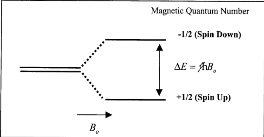
When a material containing nuclei with a net magnetic moment is placed in a magnetic field, interaction with the magnetic field results in splitting of nuclear spin states and their associated energy states. This interaction is referred to as the Zeeman interaction. For a nucleus with spin quantum number I, there are (21+1) different possible nuclear spin states when exposed the magnetic field (B, in Fig. 1.1). As illustrated in Fig. 1.1, for a spin 1/2 nucleus (when I= 1/2) such as 1H, Iz takes the value of -1/2 (spin up) or + 1/2 (spin down). In this case, the energy created by the Zeeman interaction (AE) is given by;
AE = fiB
0,
(1.1)
where *h is Plank's constant (h/2rr), and yis the gyro-magnetic ratio that relates the magnetic moment of the nucleus to its angular momentum. (For example, 7 of H is equal to 42.58 MHz/Tesla).
Magnetic Quantum Number
-1/2 (Spin Down)
_________AE ="h
0
'. _+1/2 (Spin Up)
B0
Figure 1.1 Schematic illustration of Zeeman interaction for a spin 1/2 nucleus (I= 1/2) with an external magnetic field, B0. The magnetic moment can have two states (i.e. 1/2 and -1/2),
The resonance frequency, w0, due to the Zeeman interaction is known as the
Larmor frequency, and is equal to the product of the magnetic field B, and the gyro-magnetic ratio7;
= AE /h = fiB, /=B . (1.2)
From Eq. 1.2, and given the gyro-magnetic ratio, 7/2,r = 42.58MHz / Tesla, the resonance
frequency for 'H at 1.5T is in the radiofrequency range.
The ratio of populations of down and up-spin states is determined by thermal interactions with surrounding lattice, and is derived from Boltzmann's equation as follows [42].
down -AE/kT
nup
where k is Boltzmann's constant (1.38 x 10 -3 J/K) and T is temperature. From Eq. 1.3, at
normal room temperature, the ratio is close to 10.6.
1.2.2
MR
Signal: Excitation, Precession, and Relaxation
Strictly speaking, the theoretical framework to explain the NMR phenomena involves quantum statistical mechanics, however, for simple behavior, the quantum mechanical description of nuclear resonance can be replaced by classical equations governing the procession of a magnetization vector interacting with static and time-variant magnetic fields [113]. The bulk magnetization in a volume of material, due to the Zeeman interaction, can be modeled as a magnetization vector M. M represents a magnetic moment that experiences a
torque (l') from any external magnetic fieldB, as is described by Eq. 1.4, and illustrated in Fig. 1.2.
B0
B
M
M
F=BxM
Figure 1.2 A schematic representation showing the direction of torque when the magnetization vector
M
is in an external magnetic field B (left). The torque experienced will cause a clockwise movement ofM,
rotating at the Larmor frequency, coo.F- = M
xB
(1.4)Under torque, the magnetic moment M rotates at an angular rate defined by the gyro-magnetic ratio as described by Eq. 1.5;
dM(t)
(1.5)dt F)
Combining Eq. 1.4 with Eq. 1.5, the time-varying behavior of the magnetic moment
M between external field B(t) and M(t) is represented as;
dM(t)
= 7 -M(t) x B(t) . (1.6)
dt
Equation 1.6 is solved, assuming the initial condition of
M
being tipped away from the direction ofB
by the angle a. The solution is given by Eq. 1.7. The magnetization vector M(t), where M =(M,,M,,M,), can be represented by both a longitudinal component along the z axis, MZ(t), and a transverse component rotating in the xy plane, M,, (t), where M,, (t) = M, (t) +iM
(t). MO represents the equilibrium magnitudeM, (t) = M, sin a cos(cot +
#),
M, (t) = M0sin asin(cot +
#),
(1.7)M, (t) = M,
cos a.
Let us define a frame of reference where the x and y axes rotate at the Larmor frequency around the z axis. In this rotating frame of reference, when the magnetization vector,
M,
placed in a radio-frequency (RF) magnetic field at the Larmor frequencyperpendicular to the z axis, M is rotated away from the z axis according to Eq. 1.6. This process is called 'excitation' or 'nutation'. Figure 1.3 illustrates the process. If the magnetic field,
B
1,
is oriented as shown,M
rotates about B in the clockwise direction. The angle of rotation a, is called the nutation flip angle, and is equal to a = -YB
Atr for aconstant magnitude of B, and time duration of the RF excitation, Atrf.
AZ
Mz
Y a=-yBlAtrf MMB
0MM
XFigure 1.3 A schematic drawing of the reference by the RF pulse represented by and duration of the RF pulse.
process of excitation in the rotating frame of
B
. The flip angle, a, is a function of strengthIn equilibrium,
M
is parallel to the direction of the static magnetic field B .When perturbed from their equilibrium position, the magnetization vectors in a sample will eventually relax to the initial unexcited states if there is no additional excitation. There aretwo distinct types of relaxation. One is the rate at which nuclei exchange energy with the surrounding lattice (Spin-Lattice Relaxation). The other type of relaxation is a loss of phase coherence (Spin-Spin Relaxation). The constants describing the spin-lattice relaxation and spin-spin relaxation processes are referred as T1 and T2 respectively.
The process of excitation and relaxation of the magnetization vector can be summarized by the Bloch equation obtained by adding a relaxation factor to Eq. 1.6
d M (t)
d
7t -M (t)
xB(t) - 91{M(t)-AMio}.
(1.8)
dt
B(t)
in (1.8) accounts for both the static and the RF fields(B(t)=Bo +B
1(t))
and 9iis a relaxation matrix incorporating the T, and T2 time constants;1/T2
0
0
91
0 1/T2 0 . (1.9)0 0 1 / T,
The rotating magnetization vector induces current in a coil tuned to the Larmor frequency of the specific nuclei. The detected signal magnitude is proportional to the magnitude of the transverse magnetization vector because the coil is oriented to detect the changes in transverse magnetization. The aggregates of freely precessing magnetization vectors induce a time-dependent signal referred to as the free-induction-decay (FID). The amplitude of the FID decreases over time due to loss in signal coherence. The envelope of the FID in a perfectly uniform magnetic field is represented by the decay constant T2. The
inhomogeneous nature of the physical magnetic field due to imperfection in the main magnet field or other variations resulting from susceptibility-effects due to the local field inhomogeneity [42], causes additional loss in coherence. The relaxation constant including these effects is T2'*
1.2.3 Imaging and Encoding
In order to obtain a spatial mapping of the signal sources in the sample volume after excitation, magnetic field gradients are applied to produce linear changes in the static magnetic field across the sample. Typically these linear gradients (units of Gauss/cm) are applied to the three orthogonal directions, and each coil can be energized individually or in combination so that a magnetic field gradient can be created along any arbitrary direction. With these gradients, the local Larmor frequency, co(r), is given a slight offset that is proportional to the spatial location r;
w(r)= - 7(B, + G -r), (1.10)
where r = (x,y, z) and G = (G, GY, GZ).
Equation 1.10 implies that when a gradient is applied, the spatial location along a line of the signal sources can be determined from the frequency. The next sections describe how these gradients are used in conjunction with RF excitation to encode images. We will use the example of a simple gradient echo MR sequence.
Slice Selection
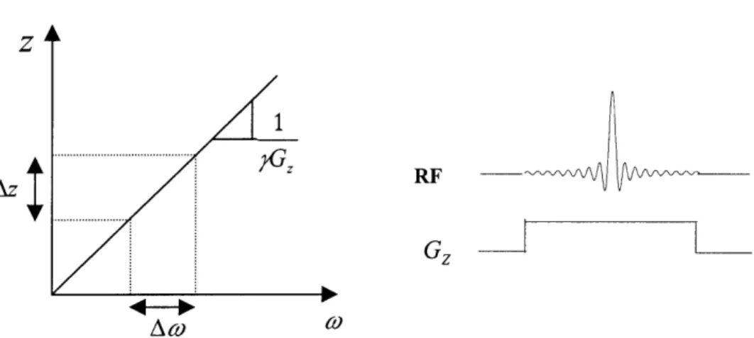
If a gradient is applied in a given direction to produce a linear variation in the Larmor frequency (Fig. 1.4), and the sample is simultaneously irradiated with an RF pulse that has a finite bandwidth (Aw in Fig. 1.4), the only excited spins will be within a single 'slab' or 'slice' of AZ = Aw that is perpendicular to that direction. Changing the carrier frequency varies the location of the slice profile whereas changing the duration of the RF pulse or the amplitude of the slice-select gradient changes the slice thickness. Time-varying gradient and RF pulses can be used to produce specialized excitation profiles for slice or volume selection [43].
1
Gz
Az
Gz
Figure 1.4 Illustration of the mapping of a finite bandwidth RF pulse (ACO)to the corresponding spatial width (Az) of spins that are excited when applying a linear gradient
G,.
Frequency Encoding
After a slab of volume in the sample is excited, assuming a homogeneous field, all magnetization vectors in the slice will initially resonate at the same frequency. We define a signal density function within the excited sample as
p(x,y)
and assume a magnetic field gradient in the x direction (G, =aB,
/ax).
Let us model the signal from a small volume atlocation x = x0 and y = yo as o(xO, yO)e-'"'. The complex exponential term
e*^' accounts for the precession due to the magnetic gradient G at location xO. The signal s(t) detected (in the rotating frame of reference) from the whole volume is,
s(t) Cc
ffp(x,
y)e -'xx"dxdy . (1.11)Equation 1.11 implies that the detected signal is proportional to the sum of signal from "columns" of material perpendicular to the x axis, and that each column resonates at a frequency proportional to its position in x, i.e., Gxx. Defining k = Gxt, an inverse
Fourier-transform on s(k) produces a function that is proportional to the projection of
,o(x,y)
along the x axis. Since the encoding utilizes the frequency for spatial indexing, it is usually referred to as "frequency encoding".Phase Encoding
The time domain signal s(t) in Eq. 1.11 can be used to obtain one-dimensional spatial information (x direction only) about the sample. An additional encoding method is necessary to provide a 2-dimensional representation of the sample. In order to achieve two-dimensional encoding, a magnetic gradient in the y direction (G, =
OB,
/ay)
is applied to modulate the phase of the excited sample p(x, y) on multiple excitations while thefrequency-encoding gradient is turned on. In order to resolve M elements in the y-direction, M "phase-encoding" steps are applied with increments of AG, made to the gradient amplitude on each step.
On each excitation, a phase encoding gradient is applied with the duration of r to create a phase offset across the volume (Fig. 1.5). Following application of the phase encoding gradient, N sets of frequency-encoded signals are obtained. For each RF excitation, a different phase encoding gradient amplitude in increments of AG, is applied, and on each of these phase encoding steps, N samples are acquired during a "readout" time at increments of AT (Fig. 1.6). The discrete set of sampled signal values S(n,m) is represented as in Eq. 1.12.
S(n,
m) c fjp(x, y)e- iy(nATGx+mAGy)dXdY , (1.12)where (-N/2+1)
n<N/2, and
(-M/2+1) m M/2.
Substituting
k
x=nATGx in Eq. 1.12 and rearranging, k, =im
rAG,S(k,,k,) Cc pfJo(x,y)e-- k dxdy . (1.13)
S(k,,
k,)
represents a sampling of the Fourier space ofp(x,y).
Therefore, from a two-dimensional inverse Fourier-transform on S(kX,k,),
we can obtain a discrete estimate or 'image' ofp(x,y). Here, k, and k, are the spatial frequencies (cm-1), and S(kx,k,)
isreferred to as the k-space representation of
p(x,y).
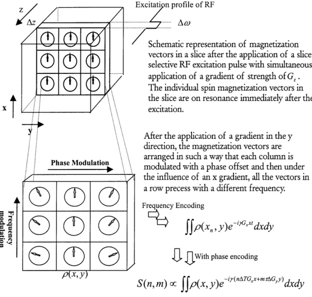
Figure 1.5 illustrates the process of slice selection, frequency and phase encoding.profile of RF
z
Schematic representation of magnetization
vectors in a slice after the application of a
slice-selective RF excitation pulse with simultaneous
.
application of a gradient of strength of G, .
The individual spin magnetization vectors in
the slice are on resonance immediately after the
excitation.
After the application of a gradient in the y
direction, the magnetization vectors are
arranged in such a way that each column is PhaseModuati modulated with a phase offset and then under
the influence of an x gradient, all the vectors in
a row precess with a different frequency.
0
~Frequency
Encodingffp(x,,
y)e-''xdxdy
GWith phase encoding
pix, y)
S(n,
m) oc
Jfp(x,
y)e i(nATGx+mrGy)dxdy
Figure 1.5 Illustration of the effect of slice selection and frequency/phase encoding to individual magnetization vectors in a sample.
Examples of MR Imaging Sequences
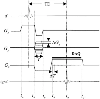
As described in the previous sections, typical MR encoding consists of slice selection followed by phase encoding and frequency encoding. Figure 1.6 shows a schematic timing diagram for a 2D gradient-echo pulse sequence. In this example, the slice selective RF pulse irradiates the sample while a slice-selective gradient (G,) is applied (from tato tb)
Following this, a phase rewinder (negative z gradient) is applied to restore a uniform phase distribution across the selected slice (from tbto t). During the same period, a
phase-encoding gradient is applied to give different phase values to the spins at different locations along the y-direction. The phase encoding gradient is varied with increments of AG, after each RF excitation. During the data acquisition period (DAQ from td to tf in Fig. 1.6), G,
is applied to produce a linear variation of frequency along the x-direction. The signal, centered at te, is sampled in intervals of AT. The magnetization vectors are all in phase at
te assuming there is no inhomogeneity in the magnetic field. The time interval between the center of the RF pulse and the center of the echo is called the echo time or TE, and the time interval between applications of each RF pulse excitation is called the repetition time or TR.
*- TE -*!
rf
Figure 1.6 Schematic timing diagram of a simple Fourier encoding sequence. The method uses a RF pulse to select the slice in the z direction with G. A
AG~ phase encoding gradient is applied
Gy after each RF excitation with the
increment of AG for the duration of
r. The MR signal is sampled while a
frequency encoding gradient is applied with sampling everyAT.
AT
Signal
Echo planar imaging (EPI), first proposed by Mansfield [44] and used widely in fMRI, allows for encoding 2 dimensional image data after a single RF excitation. Figure 1.7 shows a schematic timing diagram for a 2D gradient-echo EPI pulse sequence. First a slice is selected with slice-select gradient and RF pulse (from ta to tb) followed by a phase-rewinder (from tb to t). After the slice selection, an oscillating gradient G.,and a phase-encoding
gradient (G,) with constant magnitude are applied.
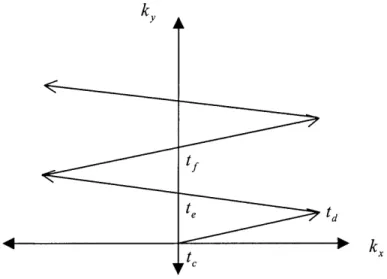
Figure 1.8 illustrates a representation of the filling of k-space by the EPI sequence in Fig. 1.7. The area under the oscillating G, and a constant G, determine the location of sampling -points k, andk, respectively (see Eq. 1.13). In the interval between t and td 5
kX is increased to its maximum. At time te, the area under the G, waveform is zero, and therefore kX = 0. At k, =0, a gradient echo is formed since the spins have maximum phase coherence with respect to action of Gx. With application of a negative value of G,,
k, reaches the minimum. G, is increased again and at k = 0, another echo is generated at time t1 . Since a constant magnitude of G is applied, k, increases with equal proportion.
The effect of the oscillating G, is the generation of gradient echoes in alternating gradient reversal periods, ,, (where r-is equal to the time interval between te and tf). EPI with
ultra-fast gradient switching, due mainly to its ability to encode a slice with a single RF excitation, is widely used for functional MRI.
Gn
Signal-ILFLT
ta tb t te td tf
Figure 1.7 Schematic timing diagram of gradient-echo planar imaging (EPI) sequence. The method uses a RF pulse to select a slice in the z direction with G,. A gradient Gx is oscillated after a single RF excitation and a constant phase encoding gradient G, is applied. The MR signal sampled fills the entire 2D k-space of a slice.
tf
te
td
'q
I
f
Figure 1.8 Representation of filling of k-space by the EPI sequence shown in Fig. 1.7.
V
-- ILY
A1.2.4 MR Signal and Contrast
MR Signal
The magnitude of the MR signal is dependent upon multiple factors such as the choice of TE, TR, and flip angle as well as the relaxation constants, T1, T2 and T2* of the
sample. Let us represent the longitudinal magnetization at time n as M" (see Fig. 1.9). Thez magnetization before and after the RF excitation are M"- and M" respectively.
flipZ=a
flipZ=a
Mj"*l) Mj"-l* M"n- M"*+
Figure 1.9 The longitudinal magnetization vector times before and after each excitation (arrow) of flip angle a.
M"~
can be derived from the Bloch equation such that [42];-TR -TR -TR -TR
Mn =M,(1-e
T )+M "-e Ti =M,(1-e Ti )+cosaM(n)~e T (1.14)In the steady state, M "- =M(n--, and Eq. 1.14 can be written as;
-TR -TR M0(1-eT )
MZ =Mj(1-(e
T1 )+cosaTie
T = (1.15)1-cosa-e
nwhere MZ is the longitudinal magnetization vector before excitation in the steady state and
a is the flip angle by which the longitudinal magnetization vector is tilted away from the z
axis (Fig 1.3).
Considering the signal detection in the transverse plane and the effect of TE (time of echo: defined in Fig. 1.6) and T2* in gradient echo sequences, the signal magnitude (S) is
-TR
S
ocN(H)e-TEIT
2*
sina Mo(I-e
T(1.16)
(1-cosa-e Ti)
where N(H) is density of
H
of the sample.From Eq. 1.16, we identify three components of the signal in gradient echo sequences. The first component is the density of 'H in the sample. The second component depends on
-TE
the ratio of TE time to T2* (e T
2
*). The third component is modulated by the effective TR
-TR
M0(1-e TI )*TeT ietognrt h
period, flip angle and the T1 of the tissue (M" = _,, ). To
Z _~~~~TR Th Etmtognrtte
1-cosa-e TI
maximum T2* weighted contrast can be shown to be at TE ~ [45]. In order to maximize
d
1
the contribution from the second factor for a fixed TR, the equation ( -TR 0
da
1-cosa-eT
is solved with respect to a. The resulting angle arE is referred to as the Ernst angle [42].
-TR
aE= Ernst angle = cos -(e ). (1.17)
Equations 1.16 and 1.17 are important for maximizing the BOLD functional signal with respect to the temporal and spatial resolution and will be used in later chapters.
MR Contrast
The relaxation constants, T1 and T2, as well as H density are different from one
tissue to another (as illustrated in Table 1.1)[42], and difference in these constants result in different signal magnitude causing contrast between tissues. Based on Eq. 1.16, which describes the MR signal magnitude for gradient echo sequences, the MR signal contrast between two different spin-bearing samples depends on the choice of TE and TR.
Tissue Ti (msec) T2(msec) Relative 1H density
White matter 510 67 0.61
Gray matter 760 77 0.69
CFS 2650 280 1.00
Table 1.1 Relaxation constants for selected tissues at 1.5T, and relative 'H density with respect to 'H density of CFS.
For example, if a small TE is used (< < 10 msec), the contribution from the term
-TE
e T2* in Eq. 1.16 is relatively small compared to the signal difference caused by the
differences in T1 of tissues if a relatively short TR is used (Ti-weighted). If a large TR is
used (TR >> 2000msec), the contribution from differences in Ti is small, and TE can be chosen so that the signal contrast is weighted toward the difference in T2* (T2*-weighted).
If TR is long and TE is short, the difference in signal magnitude is weighted primarily by the difference in H density (proton weighted).
Chapter 2
Fundamentals of Functional MRI
2.1.
Introduction
Functional MRI is an imaging technique that relates brain anatomy to the corresponding neural function. The challenge is to determine which parts of the brain are active during the performance of a certain function by measuring signals associated with the neuronal activities in brain. In the past, cognitive neuroscientists have relied on studies of laboratory animals and patients with localized brain injuries to gain insight into brain function ([46]-[48]).
Functional imaging of the human brain has been performed by detecting radiation decay of single photons emitted from radioisotope-labeled pharmaceutical agents in Single Photon Emission Computer Tomography (SPECT) or the radiation due to pairs of photons created by annihilation of positron-electron-pairs in Positron Emission Tomography (PET). However, these techniques are invasive due to the need to inject radioactive isotopes [50, 51]. Non-invasive techniques such as EEG (ElectroEncelphaloGraphy) and MEG (Magneto-Encelphalo-Graphy) have been used to map the source of electrical and magnetic fields associated with neuronal activation in high temporal resolution. However, the inverse solution for source localization is inherently inaccurate [52, 53], and spatial resolution of the methods is low, on the order of a centimeter [52].
Functional MRI (fMRI) can be used to detect the intrinsic signal changes caused by blood oxygenation level, local cerebral blood flow (CBF) and cerebral blood volume (CBV) during neuronal activity in the brain. fMRI enables the examination of human cortical function without the use of radioactive contrast agents and with reasonable temporal and spatial resolution. In the following sections, we review the contrast mechanisms and basic physiological foundations of functional MRI along with the current MR sequences and methods used.
2.2. Contrast in fMRI
2.2.1 Physiological Basics in Neuronal Activation
From functional studies such as direct action potential measurement and optical imaging using an infrared light source [54,56], neuronal activity is found to take place with delays in the range of 100's of milliseconds between stimulus presentation and neuronal response for most of the brain regions [52]. Functional MRI detects changes in the perfusion-state modulated by the neuronal activity of the brain. Hemoglobin, the oxygen-carrier in blood, acts as a shuttle to deliver oxygen after binding to the oxygen. Hemoglobin bound to the oxygen is called oxygenated-hemoglobin (also known as oxyhemoglobin) whereas the oxygen-depleted form of hemoglobin is called deoxygenated-hemoglobin (deoxyhemoglobin). The concentration of local oxyhemoglobin and deoxyhemoglobin is determined by cerebral blood flow (CBF), cerebral blood volume (CBV), and local oxygen consumption [55,56].
During neuronal activation, neuronal cells require extra energy, and their oxygen consumption increases. Oxygen supplies are provided to neuronal cells via perfusion and diffusion, however, the exact physiological mechanism is still unclear [34, 55, 56]. Increase in oxygen consumption leads to an increase in local CBF. As CBF increases, the local tissue and vascular compliance in the brain determine the local CBV. The supply of oxygen eventually overcompensates for the initial increase in oxygen consumption. As a result, there is an increased concentration of oxygenated hemoglobin with respect to the deoxygenated hemoglobin (hyperoxemia) [56].
2.2.2 Contrast Mechanisms in Functional MRI
Exogenous paramagnetic contrast agents such as gadolinium or dysprosium compounds have been used to relate changes in CBF and CBV to signal contrast in MRI. These contrast agents are paramagnetic and create a local magnetic inhomogeneity, which results in a local phase variation. If there is significant phase variation within a voxel, there will also be significant amount of phase-cancellation within a voxel [55,59]. This intravoxel-dephasing results in loss of signal in T2* weighted imaging sequences.
By injecting a bolus of these paramagnetic contrast agents into the bloodstream, changes in CBV and CBF during neuronal activity can be measured. For example, according to the work of Rosen et al. [4], an intravenous administration of a bolus contrast agent, induces transient reduction in T2 or T2* weighted signal and changes in intravascular
concentration of the contrast agents can be estimated by the signal reduction. By integrating the concentration-time curve and normalizing to the integrated arterial input data, CBV has been estimated. CBF is quantified from the change in CBV normalized to the estimated mean-transit time of contrast agents in the region. However, injected contrast agents have to be cleared from the blood stream before the new sets of data are obtained, therefore, repeated data acquisition is limited. In addition, the injection of exogenous contrast agents is an invasive procedure.
An approach that does not depend on the injection of exogenous contrast agents is spin labeling, [57]. Water protons from in-flowing arterial blood can be labeled using spin-saturating RF pulses. From Echo Planar imaging and signal targeting with alternating RF (EPISTAR), maps of changes in CBF can be created by subtracting two sets of data acquired alternatively with and without a 1800 inversion applied to the proximal region of arteries. However, the technique is limited to the imaging of one slice per scan. This mechanism, detecting activation via changes in cerebral blood flow, is referred to as flow-related enhancement (FRE).
2.2.3 BOLD Contrast
Local changes in the state of oxygenation can also be detected by the Blood Oxygenation Level Dependent (BOLD) contrast mechanism. The basis of the BOLD technique is that deoxyhemoglobin acts as an endogenous paramagnetic contrast agent and therefore, changes in its local concentration lead to the variation in T2 or T2* weighted MR
images ([55],[58]-[62]). As hemoglobin (Hb) becomes deoxygenated, it becomes more paramagnetic than the oxygenated Hb and thus creates a magnetically inhomogeneous environment. The signal increase in T2 or T2* weighted images acquired during cortical
activation reflects a decrease in deoxyhemoglobin content, i.e., an increase in blood oxygenation. The blood hemoglobin paramagnetism decreases with brain activation and the local CBV increases. The resulting decrease in tissue blood magnetic susceptibility differences leads to less intra-voxel dephasing within cortical tissue and hence increased intensity level in appropriately weighted images [55]. Because BOLD contrast does not require the injection of contrast agents and multi-slice acquisitions are possible, it is most widely used for fMRI today [62].
Blood oxygenation level dependent (BOLD) contrast varies according to the type of sequence used in the experiment. Gradient-echo sequences are most sensitive to the changes in local T2* whereas spin-echo sequences are most sensitive to the T2 variations
associated with BOLD effects.
Gradient Echo Sequences
Similar to the case where an exogenous paramagnetic contrast agent is present, the susceptibility difference results in local inhomogeneity due to BOLD effect and creates a phase variation of blood with respect to the surrounding tissue. If this phase variation is distributed over the size of a voxel, there can be a significant amount of phase-cancellation within the voxel (intravoxel-dephasing), resulting in the loss of intensity in T2*-weighted
images. Based on the magnitude of MR signal described in Eq. 1.16, the signal contrast (AS) between activated and baseline states becomes,
AS
=
Soe-TE.R
2*BAs(e TE-AR*2 _1),(2.1)
where R* is the transverse relaxation rate (I/T2*BASE ) in baseline states and AR* is the transverse relaxation rate (1/T2*) due to the activation. So represents the initial baseline signal. When TE -AR* <<1, the above equation can be approximated as;
AR
AS / S
AR
2T~-
TEE
(2.2)
Since the different dimensions and orientations in the vessel types (vein, venuoles, and capillary), and physiology (such as recruitment and dilations) affect the intra-voxel phase dispersion, it is difficult to exactly quantify the phase change due to BOLD activation. However, mathematical models suggested that the degree of contribution from the larger vessels (AR; = -3.4 s-') is greater than from the capillary-based tissue (AR* <-1s-1) [61]. Gati et al. investigated the percentage change due to BOLD effect, and estimated AR* for the both vessel and tissue [22], which agreed well with the theoretical value by Boxerman et al [61]. According to their work, up to -18% of signal change is expected in the vessel whereas only -2% is expected from the tissue at 1.5 T. Using high magnetic field environment at 4.OT, Menon et
al.
[56] reported that a large portion of the signal changes that accompany photic stimulation comes from capillary-containing tissues that are not visible in lower field. In gradient-echo experiments at 1.5T, the dominant source of signal is from the draining veins [62, 63].Spin-Echo Sequences
The BOLD contrast obtained with spin-echo sequences is considerably smaller than that obtained using gradient echo sequences [65,67]. The BOLD contrast elicited by changes in the transverse relaxation rate, AR , in spin-echo sequences is smaller than changes due to AR* with gradient-echo sequences by a factor of -0.3 at 1.5T[65]. However, in spite of the smaller changes in transverse relaxation rate, spin-echo sequences are a serious alternative for fMRI experiments because, unlike gradient echo sequence
where the dominant source of signal is from the large draining veins, BOLD contrast arising from the spin-echo sequences more likely reflects change of oxygenation in microvessels such as capillaries [60,63],
It has been shown that spin-echo sequences are sensitive to the BOLD effect due to the random motion of water molecules in the extravascular space [65,66]. The presence of magnetic field gradients at the interface between blood vessels and surrounding tissue will result in MR signal loss [55,61]. Several biophysical models accounting for these factors predict that resulting transverse relaxation rate, AR , in spin-echo sequences are more sensitive to regions around vessels of small radius (dimension similar to capillary diameter in the order of 2-7 p.#n) than regions associated with large vessel radius [55,64,65].
Spatial and Temporal Characteristics
The neuronal activation is known to occur at the site of single or groups of neurons that are responsible for certain functional sub-units and these sub-units overlap each other to form functional units [56, 68]. For instance, the functional subunit for ocular dominance is determined by an area (Ocular Dominant Columns), typically 5-10mm in length and 0.8-1.2mm on a side, however, the functional unit as a whole may extend to centimeter long columns [56]. Similar observations have been reported for the study of somatotopy in hand motor-area with overlapping areas of sub-units responsible for the movement of individual digits [10] and for study of bilingual generation with overlapping areas for different languages [26]. The minimum detectable size of functional activity at 1.5T is well under a millimeter, based on the various studies where data was acquired at high spatial resolution [26,60,63].
In terms of the temporal characteristics in BOLD activation, images can be collected in a very short time using fast imaging sequences therefore, high temporal resolution is possible in principle. The hemodynamic response, on the order of 2 to 3 seconds, lags behind the time of neuronal activity. However, in spite of the delay in hemodynamic response, high temporal resolution is desirable to resolve the sequential involvement from the multiple cortical areas and the associated hemodynamic responses [34, 69, 70].


![[PDF] Objective Caml cours facile pour débutant | Formation informatique](data:image/gif;base64,R0lGODlhAQABAIAAAP///wAAACH5BAEAAAAALAAAAAABAAEAAAICRAEAOw==)