HAL Id: hal-02558529
https://hal.archives-ouvertes.fr/hal-02558529
Submitted on 4 May 2020
HAL is a multi-disciplinary open access
archive for the deposit and dissemination of
sci-entific research documents, whether they are
pub-lished or not. The documents may come from
teaching and research institutions in France or
L’archive ouverte pluridisciplinaire HAL, est
destinée au dépôt et à la diffusion de documents
scientifiques de niveau recherche, publiés ou non,
émanant des établissements d’enseignement et de
recherche français ou étrangers, des laboratoires
vortex zones along a labyrinth milli-channel used in drip
irrigation
Jafar Al-Muhammad, Séverine Tomas, Nassim Ait-Mouheb, Muriel Amielh,
Fabien Anselmet
To cite this version:
Jafar Al-Muhammad, Séverine Tomas, Nassim Ait-Mouheb, Muriel Amielh, Fabien Anselmet.
Ex-perimental and numerical characterization of the vortex zones along a labyrinth milli-channel
used in drip irrigation.
International Journal of Heat and Fluid Flow, Elsevier, 2019, 80,
International Journal of Heat and Fluid Flow 00 (201 ) 1–25
Heat and
Fluid Flow
Experimental and numerical characterization of the vortex zones
along a labyrinth milli-channel used in drip irrigation
Jafar Al-Muhammad
a,b,⇤, S´everine Tomas
a, Nassim Ait-Mouheb
a, Muriel Amielh
b,
Fabien Anselmet
baG-EAU, AgroParisTech, Cirad, IRD, IRSTEA, MontpellierSupAgro, Univ Montpellier, Montpellier, France
361 rue Jean-Franc¸ois Breton, BP 5095, 34196 Montpellier, cedex 5, France
bIRPHE UMR 7342, Aix Marseille Universit´e - CNRS - ´Ecole Centrale Marseille
49 Rue Fr´ed´eric Joliot-Curie, BP 146, 13384 Marseille, Cedex 13, France
Abstract
The labyrinth-channel is largely used in dripper systems. The baffles play an important role to generate the head losses and induce the flow regulation on the drip irrigation network. But they also develop vorticity regions where the velocity is low or zero. These vorticity regions promote the deposition of particles or other biochemical development causing dripper clogging. The flow in the dripper labyrinth-channel must be described to analyze dripper clogging sensibility which drastically reduces its performance. This characterization is performed experimentally using the micro-particle-image-velocimetry (Micro - PIV) method, and numerically using the RSM Simulation. In this study, Micro-PIV experiments allow to analyze the flow in ten-pattern repeating baffles which reproduce the micro-irrigation dripper. The cross section is equal to 1 mm2and the inlet Reynolds number varies from 345 to 690. The present study first introduces a global analysis of the flow through the mean velocity modulus, the Reynolds stresses u02, v02and u0v0and the turbulence Reynolds number. Then, results for the mean strain rate and the mean spanwise vorticity are presented and discussed. Next, advanced methods of vortex detection are introduced and analyzed to better distinguish the vortex zones and to determine the vortex sizes. Furthermore, the numerical model is used to validate and analyze in a more detailed way the experimental results obtained by Micro-PIV.
Keywords: Drippers, Labyrinth micro-channel, Micro-PIV, RSM model, Vortex identification
⇤Corresponding author: Tel.: +33-6-18187649, Fax: +33-4-67166492
Email address: almuhammadj@gmail.com (Jafar Al-Muhammad)
1. Introduction
Drip irrigation is a technique characterized by low-velocity water flows. Water drops near the plants through drippers. This type of irrigation improves efficiency by reducing evaporation, drift, runoff and deep percolation losses when compared with the other techniques such as sprinkler irrigation. In this technique, drippers are the most important and critical components (Karmeli, 1977 [20]). Drippers generate low flow rates between 0.5 and 8 [l.h 1] for pressure between 50 and 400 kPa (Goldberg et al., 1976 [15]). Dripper flow rate increases with static pressure in a lateral pipe according to a power-law (Karmeli, 1977 [20]): q = kdPx, where q is the dripper flow rate [l.h 1], kdthe proportionality coefficient that characterizes each dripper, P the working pressure head at the dripper [Pa] and x the dripper discharge exponent. The value of this exponent depends on dripper conception. This relationship determines the dripper performance. Indeed, manufacturers try to design drippers whose flow rate is not directly dependent on the pressure head (x < 0.5). To reach this goal, they introduce some elements in the dripper such as a labyrinth-channel which generates local pressure head losses. Drippers can be divided into two categories: pressure compensating and non-pressure compensating drippers. Pressure compensating drippers are provided with a membrane by which the flow control is achieved. This category provides the same amount of water all the way down the slope. Non-pressure compensating drippers use long tortuous channels which provide greater durability and longevity along with clogging resistance and low maintenance thanks to the absence of moving parts.
The labyrinth-channel section is in the order of 1 [mm2], so baffles are likely to be clogged by physical particles not captured by the filtering system. As a result, the irrigation uniformity is perturbed and the investigation cost is increased (Pitts et al., 1990 [31]) due to maintenance needs and durability decrease.
Some studies have been performed to analyze the dripper clogging and performance. They indicate that clogging occurs in low-velocity vortex regions as it was experimentally found (Zhang et al. 2007 [38]; Wei et al. 2012 [34]; Ait-Mouheb et al. 2019 [1]). When designing drippers, clogging can be prevented or at least significantly reduced by decreasing, as much as possible, the vortex size. Thus, anti-clogging properties and consequently drip irrigation efficiency are strongly related to hydraulic performance. The flow characterization inside the labyrinth-channel is difficult to examine by experimental methods due to the small size and intricacy of drippers (Zhang et al., 2007 [38]). Therefore, numerical modeling is also helpful to study the flow in the labyrinth-channel. Several numerical studies emphasize that dripper performances are related to hydraulic conditions (Berkowitz, 2001 [6]; Li et al. 2008 [27]; Palau et al. 2004 [30]). From these studies, one can also infer that the choice of a numerical model is not fixed. Indeed, the standard, RNG (Re-Normalisation Group) and realizable k e models as well as the RSM model (Reynolds Stress Model) were used without clear justifications.
A few experimental studies have been performed to analyze the labyrinth-channel and to compare with the modeling. The particle image velocimetry (PIV) was used by Li et al. (2008 [27]) to assess flow characteristics in the labyrinth flow path. Then, Li et al. (2008 [27]) compared experimental results with numerical ones obtained with the k e model as turbulence model. The Micro-PIV technique was also used by Wei et al. (2012 [34]) to visualize the
water flow with suspended sand particles inside the labyrinth-channel under the pressure range 40-150 [kPa] on two geometries. They used the RNG k e model to perform simulations and conclude that Computational Fluid Dynamics (CFD) simulation results show reasonable agreement with their experimental results on the basis of the curve for the pressure-discharge relationship. Particle Tracking Velocimetry (PTV) was employed by Yu et al. (2017 [37]). Three clay particle diameters were studied: 65, 100 and 150 [µm]. They employed CFD-DEM (Discrete Element Method) to perform the numerical work. The unsteady Standard k e model was used as turbulence model. Nevertheless, only the velocity (of the liquid or the solid phase) and the position of sedimentation regions were analyzed.
However, a recent study performed by Al-Muhammad et al. (2018 [4]) has shown that the flow in the labyrinth-channel is anisotropic (i.e the turbulence is different in the three spatial directions (Pope, 2000 [32]). Therefore, models that assume isotropic turbulence should not be selected anymore to model such a flow. But, the standard k-e model and its variants (k-e RNG, k-e realizable) do not take into account the flow anisotropy (Al-Muhammad et al., 2016 [3]). That is why, in the present study, a more complex model such as RSM is considered to simulate properly this flow as an equation is solved for each of the Reynolds stresses. Also, we propose to overcome the difficulty of experimental measurements for a geometry such as the labyrinth-channel by an advanced optical technology. This consists in performing Micro-PIV experiments (Al-Muhammad et al., 2018 [4]). As far as we know, it was the first time that such a Micro-PIV technique was developed to determine with high accuracy, compared to the other studies in the irrigation domain, the mean and fluctuating velocity fields inside the labyrinth-channel constituting irrigation drippers. Herein, these experimental results will be compared with RSM simulations to analyze the flow within the labyrinth-channel. Firstly, the velocity fields and profiles are presented along the labyrinth-channel, and then, the turbulence properties of the flow are presented and discussed. Next, a detailed analysis based on the definition of the vorticity is introduced. Finally, advanced methods such as thel2and Q-criteria are used to detect and characterize the vortex zones in the labyrinth-channel flow. Such an analysis is also important for passive micro-mixer subsystems where mixing enhancement is a crucial issue (Capretto et al., 2011 [7]).
2. Materials and methods 2.1. Case study
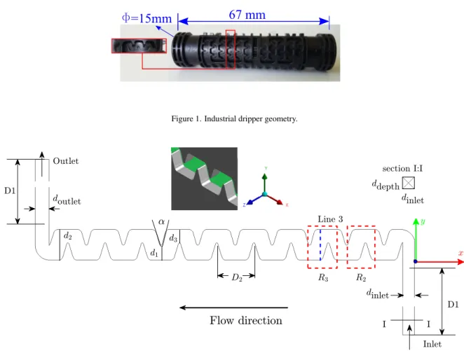
The dripper chosen is an integrated one with non-uniform section which produces a turbulent flow. This dripper is that most widespread in drip irrigation. It is displayed in Fig.1. The dripper is composed of 60 baffles (labyrinth-channel units). Each three baffle pattern composes the basic unit which is repeated 20 times. This is the dripper least sensitive to clogging (see Al-Muhammad 2016 [2] for more details). A detailed geometry in 2D, with all dimensions, of the presently studied labyrinth-channel is shown in Fig.2. All the dimensions are presented in table1. For Micro-PIV, it is exactly the ten-pattern channel that is studied. For RSM simulations, only three baffles are considered, as the flow is then developed (Al-Muhammad et al., 2018 [4]).
67 mm
F=15mm
Figure 1. Industrial dripper geometry.
Figure 2. Ten baffle labyrinth-channel used in micro-PIV present experiments. Only the three first baffles are used to perform RSM modeling. The inlet and outlet conditions are the same in the experimental and numerical studies. The blue-colored line and rectangles R2and R3represent the
zones where the results will be analyzed. The line 3 coordinates are x = 8.5 [mm], y = 0 2.80 [mm], and z = 0.575 [mm].
Experiments have been performed with three flow rates 24 [ml.min 1] (1.44 [l.h 1]), 36 [ml.min 1] (2.16 [l.h 1]), and 48 [ml.min 1] (2.88 [l.h 1]), where the minimum and maximum flow rates are chosen symmetrically around 2.16
Table 1. The presently studied labyrinth-channel dimensions.
Inlet width dinlet 1.20 mm
Outlet width doutlet 1.40 mm
Depth ddepth 1.15 mm d1 1.35 mm d2 2.80 mm d3 1.35 mm D1 10.00 mm Unit length D2 3.24 mm Hydraulic diameter Dh 1.17 mm Angle a 33 o
[l.h 1]which corresponds to the nominal flow rate of such a dripper. These flow rates correspond to Reynolds numbers Re`of 345, 510 and 690. Re`is defined as
Re`=r ·|u|inletµ · Dh, (1)
whereµ is the dynamic fluid viscosity [kg.m 1.s 1],r is the fluid density [kg.m 3], |u|
inletis the bulk velocity at the inlet, defined by the equation: |u|inlet=q/(dinlet⇥ ddepth), with dinletthe inlet width and Dhthe hydraulic diameter. 2.2. Experimental method
The 2D-2C Micro-PIV set-up is composed of a laser source (Litron Nd-YAG Laser of 135 mJ, doubled in fre-quency (532 nm)) and a HiSense 4M camera. The Dantec Dynamics HiSense 4M camera offers high resolution (2048 ⇥ 2048 pixels) combined with high sensitivity, with a pixel size of 7.4[µm]. This camera is equipped with a Canon MP-E 65 mm f /2.8 lens. Three extension rings (extension tubes) of 12, 20 and 32 [mm] have been added to increase magnification up to 6.9 and thus to visualize 1[µm] PIV particles.
Time delays between two laser pulses within a pair are 12 and 6[µs] for Re`=345 and Re`=690 respectively. In other word, this is the time between two frames which provides one velocity field. The acquisition frequency, between two pairs of images, is 1 [Hz]. Seeding particles of 1[µm] are selected to perform the Micro-PIV experiments. Fields of view are 2.2 ⇥ 2.2 [mm] and the treatment is realized with 32 ⇥ 32 pixels as interrogation window. An overlapping of 50% is applied. The final spatial resolution, thus, becomes 16 ⇥ 16 pixels. The experimental set-up settings are explained, detailed and validated in Al-Muhammad (2016 [2]) and Al-Muhammad et al. (2018 [4]). All the technical parameters and calibration of Micro-PIV experiments are described therein. The correlation depth has thus been esti-mated to be 82[µm] which means that the velocities are averaged over this depth.
The measurement uncertainty strongly depends on both the particle-image diameter dtand the uncertainty in locating the image centroid represented by c. dt is defined as:
dt= q
(M.dp)2+ddiff2 (2)
and
ddiff=2.44 f#l(M + 1) (3)
In the present experiments, f#=2.8, with wavelengthl = 532 nm, the image magnification M = 7.7 and dp=1µm. When replacing in Eq.2, we find dt =32.55µm. As it is found by Prasad et al. (1992 [33]) if a particle image diameter is resolved by 3-4 pixels, the location of a particle-image correlation peak can be determined to within 1/10ththe particle-image diameter. The measurement uncertainty is then ofdx ⇡ d
t/10M which gives an error of about 0.42µm. Next, the effects of the local velocity gradients is studied by Westerweel (2008 [36]). In some study, this effect can be ignored when the variation a of the local particle-image displacement is small with respect to dt. i.e. a ⌧ dt , a = MDu Dt where Dt is the exposure time delay, and Du represents the local variation of the velocity field,
i.e., |Du| ⇠ |∂u/∂x| · L where L is a typical dimension of the interrogation window size.
The random errorsDxis proportional to the width dDof the displacement-correlation peak, and for a simple shear it is approximately given by:
sDx c dt r
1 +2
3a2/dt2 (4)
with c = 0.05 7 (Westerweel, 2008 [36]). In the present study, dt=32.55µm, L = 34.4µm, |∂u/∂x| = 3745 s 1 for Re`=690 which give :sDx=1.46 205µm. From the instantaneous velocity fields obtained by Micro-PIV, the velocity modulus |u|, the velocity fluctuations about the mean (u0and v0) are derived and calculated.
|u| = pu2+v2 (5)
This formulae can be applicable for the mean velocity (u) instead of instantaneous velocity (u) to find |u|, and
u0=u u (6)
and
v0=v v (7)
Several statistical quantities are calculated from ensembles of instantaneous velocity fields containing the mean x and y velocity components (u and v), the second-order moments of the fluctuating velocities u02, v02and u0v0and the mean velocity modulus |u|. These statistical quantities serve to calculate the convergence residues. While the final statistical quantities which serve to plot and calculate the velocity fields and vectors are calculated from:
uj(x,y) = 1 Nv Nv
Â
k=1 ujk(x,y) (8) j=1,2 |u(x,y)| = N1 v NvÂ
k=1|uk (x,y)| (9)where k is the running image number, Nvis the number of valid images (around 700 in our case) which is different from the total number of images N (750).
The second-order moments of velocity fluctuations are defined as: u0 iv0j(x,y) =N1 v Nv
Â
k=1 ⇣ uik(x,y) ui(x,y) ⌘ ⇥⇣ujk(x,y) uj(x,y) ⌘ (10)i and j=1,2.
The second-order moments of fluctuating velocities residues are calculated by the formula:
Ru0iu0 jNv= 1 Nv Nv  k=1u 0 iku0jk 1 Nv 1 Nv  k=2u 0 ik 1u0jk 1 2 1 Nv Nv  k=1u 0 iku0jk 2 , (11)
where : i, j = 1,2 and for (x,y).
These residue values are globally about 10 7for the u and v velocities and 10 6for the second-order moments of fluctuating velocities u02and v02. For u0v0, the residues can not decrease lower than 10 5because the denominators of the residue formula are generally closer to 0 (about 10 4) (see Al-Muhammad et al. (2018)[4] for more details).
2.3. Turbulence model for the fluid flow
In this study, incompressible steady-state flow is assumed. Buoyancy and gravity are not taken into account. For a turbulent flow, the fluid motion can be described by the mean continuity equation, mean momentum equation, the exact transport equation for the Reynolds stress tensor, the turbulent kinetic energy (k) equation and the turbulent dissipatione equation. For the mean velocity field, the continuity and Navier-Stokes equations write:
∂ui ∂xi =0 , (12) r∂x∂ j(uiuj) = ∂ p ∂xi+ ∂ ∂xj µ✓ ∂u∂xi j+ ∂uj ∂xi ◆ + ∂ ∂xj h ru0 iu0j i , (13)
where i and j are indices denoting Cartesian coordinate directions, ui and uj are the mean velocities [m.s 1], p is the mean pressure [Pa], and u0
iand u0j are the velocity fluctuations [m.s 1]. The additional term, the Reynolds stress tensor, Ri j=ru0iu0j, needs to be modeled. The Reynolds Stress Transport Model, (RSM-LRR) derived by Launder et al. (1975 [25]), is chosen herein to simulate the flow in the labyrinth-channel. This model closes the Reynolds-averaged Navier-Stokes equations by solving additional transport equations for the Reynolds stresses Ri j, together with an equation for the dissipation ratee.
Since the RSM can account for the effects of streamline curvature, swirl, rotation and rapid changes in strain rate, it has greater potential to give accurate predictions for complex flows such as that for the labyrinth-channel. The symbolic form of the exact transport equations for the Reynolds stress tensorru0
iu0jmay be written as follows: Ci j |{z} Convection = DT,i j | {z } Turbulent diffusion + DL,i j | {z } Molecular diffusion + Pi j |{z} Stress production + fi j |{z} Pressure strain ei j |{z} Dissipation (14) 7
The terms that do not require modeling are Ci j, DL,i j and Pi j. While, the other terms, DT,i j,fi j andei j need to be modeled to close the equations. The turbulent diffusion DT,i jis usually modeled using a scalar turbulent diffusivityµt (Lien and Leschziner, 1994 [28]). The modeling of pressure-strain term,fi j, is composed from several terms (Chou, 1945 [9]), and is modeled on the basis of the proposals of Gibson and Launder (1978 [14]), Fu et al. (1987 [12]) and Launder (1989 [24]).
Dissipation terms are obtained with the usual assumption that:
ei j=23redi j (15)
The value ofe is obtained by solving the following modeled equation: ∂ ∂xi(reui) = ∂ ∂xj ✓ µ +sµt e ◆ ∂e ∂xj + 1 2Ce1Gk e k Ce2r e2 k (16)
wherese =1.00, Ce1=1.44 and Ce2=1.92. Gk=µtS2represents the production of turbulent kinetic energy, with µt the turbulent viscosity defined asµt=rCµke2 with Cµ=0.09, and S the modulus of the mean rate-of-strain tensor, which is defined as S = q2Si jSi j(Si j=12(∂u∂xij+
∂uj
∂xi)). 2.4. Numerical approach and boundary conditions
The study is performed using the commercial computational fluid dynamics software ANSYS/Fluent V14. Sim-ulations are performed in three dimensions (3D). The mesh is generated and its quality is examined. A prism with quadrilateral base mesh type is adopted. The skewness, based on the deviation from a normalized equilateral angle, is around 0.56 which states that mesh quality is acceptable. The independence of the results to the meshing has been verified (see Al-Muhammad (2016 [2]) for more details). The mesh is constructed to satisfy y+<5 (where y denotes here the distance to the wall of the first mesh point, normalized by the friction velocity and the kinematic viscosity). Enhanced wall treatment is used to model the near wall region. When using enhanced wall treatment as the near-wall treatment, zero flux wall boundary conditions to the Reynolds stress equations are applied. The RSM model requires boundary conditions for turbulence quantities (k ande) and individual Reynolds stresses ru0
iu0j. k ande can be input directly or derived from the turbulence intensity and a characteristic length. This last method is chosen; low turbulence intensity (5%) with a hydraulic diameter Dh=1.17 [mm] (see table1) are chosen for the specification method. The turbulent kinetic energy (k) and turbulent intensity are, then, selected for Reynolds-Stress Specification method. To solve the pressure-velocity coupling and to interpolate face pressure, we choose respectively the SIMPLE and STANDARD methods which are robust and valid for a large flow range. Third-order MUSCL discretization is selected to solve the momentum, Ri jand dissipation rate equations because this method is accurate and adapted for all mesh types. Least Squares Cell-Based is the method used to calculate gradients. This method calculates gradient values using adjacent surface cells. Its accuracy is higher than the Green-Gauss Cell-Base method and its cost is lower than
C0 Ci ri
Figure 3. Cell Centroid Evaluation, extracted from User’s guide ANSYS/Fluent 14.0.
the Green-Gauss Node-Based method both available in ANSYS/Fluent. As a majority of the results discussed in sec-tion4are based upon the differential quantities, it is necessary to present in detail the schemes of gradient calculation. The Least Squares Cell-Based method approximates the gradient at the center of each cell using the least squares approximation. The derivatives in each cell are assumed to change linearly along the separating distances of all the neighboring cells. In Fig.3the change in cell values between cell C0and Cialong the vector ~rican be expressed as (User’s guide ANSYS/Fluent 14.0):
(—f)(c0)· Dri= (fci fc0) (17)
when applying Eq.17for all cell surrounding the cell c0, we obtain the following system :
[J](—f)(c0)=D(f) (18)
Where [J] is the coefficient matrix which depends purely on geometry.
Then, Eq.18can be solved by decomposing the coefficient matrix using the Gram-Schmidt process [5]. This decom-position yields a matrix of weights for each cell wi0. Therefore, the gradient at the cell center can then be computed by multiplying the weight factors by the difference vector,
—(fj)(c0)= N
Â
i=0wi0j(fci fc0) (19)
where j= 1, 2, 3; N is the number of neighboring cells; and wjthe weighting factors of neighboring cells. The gradient schemes are presented in detail by Mishriky and Walsh (2017) [29].
3. Flow characteristics of labyrinth-channel dripper 3.1. Mean velocity modulus field
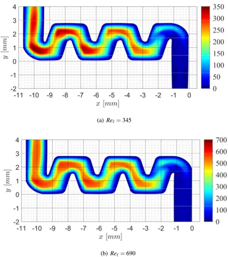
Mean velocity modulus fields obtained experimentally by the Micro-PIV technique and numerically by the RSM model are compared in Fig.4 where streamlines colored by mean velocity modulus are plotted for Re`=690. The
blue-colored zone, in the mean velocity fields, allows having a global overview on the vortex zone formed inside the labyrinth-channel flow. This vortex zone is characterized by low-velocity values. The RSM model predicts approxi-mately the same vortex zone form as Micro-PIV does, even if the vortex center is not exactly at the same position and velocity magnitude is greater for the Micro-PIV results : 1.65 and 1.55 times greater at y/d2=0.1 for Re`=345 and Re`=690 respectively (Fig.5). The estimation error can be related to the effects of the local velocity gradients which depends strongly on c (Eq.4). The parameter c depends on several parameters among it the seeding particles number in the interrogation window (Westerweel, 2000 [35]). This number is not well controlled in the vortex zone when the micro-PIV experiments are performed in view of the geometry complexity.
(a) Micro-PIV (b) RSM model
Figure 4. Velocity streamlines in the rectangle 2 (see fig.2) for Re`=690.
0 0.2 0.4 0.6 0.8 1 0 0.5 1 1.5 2 2.5 (a) Re`=345 0 0.2 0.4 0.6 0.8 1 0 0.5 1 1.5 2 2.5 (b) Re`=690
Figure 5. Normalized mean velocity profiles : comparison between Micro-PIV (blue) and the RSM model (red) along the line 3, for Re`=345 and
Re`=690.
Normalized mean velocity profiles along line 3 (Fig.2) are plotted in Fig.5to investigate with more accuracy this comparison and analyze the differences. The numerical results are close to the experimental data for both Reynolds numbers. The model over-predicts the velocity in the mainstream flow, characterized by high flow velocity, for
Re`=690 by 5% in comparison with the experimental values. However, an important difference is remarked in the vortex zone, characterized by low flow velocity, where the model under-estimates the mean velocity modulus with 75% in comparison with the experimental values. Indeed, the form of the vortex zone is slightly changed. Numerically, the vortex zone center is closer to the wall with a weak velocity value in comparison with Micro-PIV data. However, the mean velocity modulus does not allow to determine precisely the vortex zone and mainstream flow, therefore, a specific analysis is conducted in section4.
3.2. Reynolds stresses
The objective of this paragraph is to study and to compare experimentally and numerically, the Reynolds stresses u02, v02and u0v0. The experimental Reynolds stresses are presented and discussed by Al-Muhammad et al. (2018 [4]). The Reynolds stress profiles are presented in Fig.6and Fig.7for Reynolds numbers 345 and 690 respectively.
0 0.2 0.4 0.6 0.8 1 0 0.2 0.4 0.6 0.8 (a) u02 0 0.2 0.4 0.6 0.8 1 0 0.2 0.4 0.6 0.8 (b) v02 0 0.2 0.4 0.6 0.8 1 -0.6 -0.4 -0.2 0 0.2 0.4 (c) u0v0
Figure 6. Normalized Reynolds stress profiles along the line 3 for Re`=345.
0 0.2 0.4 0.6 0.8 1 0 0.2 0.4 0.6 0.8 (a) u02 0 0.2 0.4 0.6 0.8 1 0 0.2 0.4 0.6 0.8 (b) v02 0 0.2 0.4 0.6 0.8 1 -0.6 -0.4 -0.2 0 0.2 0.4 (c) u0v0
Figure 7. Normalized Reynolds stress profiles along the line 3 for Re`=690.
Reynolds stress u02is well predicted by the RSM model when comparing with Micro-PIV results for Re`=690. However, the Micro-PIV experiments attenuate the fluctuating quantities near the wall and in high gradient regions. The effects of the spatial attenuation on the measured turbulence statistics in the wall vicinity, in PIV experiments, are assessed and reported by Kahler et al. (2006) [21] and Lee et al. (2016) [26]. Some deviations appear due to volume averaging in the wall region: Lee et al. (2016) [26] show that, with the assumption that the small-scale contributions to the fluctuating velocity variances do not depend on the Reynolds number, some universal corrections can be applied.
This procedure was developed for canonical flat plate turbulent boundary layers at quite large Reynolds numbers Ret (where Retis computed with the boundary layer thickness and the friction velocity), Ret= [900 2600], and for quite large interrogation windows (Dx+' Dy+>20). In our case, the interrogation window size isDx = Dy = 34.4µm, corresponding toDx+=Dy+' 3.5, which is likely to induce negligible attenuation effects according to the figure 8 presented in Lee et al. (2016) [26]. In addition, our configuration is far from a canonical turbulent boundary layer due to the labyrinth geometry and the Reynolds numbers are small (Ret = [60 85]). Therefore, no correction to account for the effect of the interrogation window size was applied in the present study. There are some differences between the micro-PIV and the RSM results for v02 in the transition between the mainstream flow and the swirl zone (y/d2=0.4 0.7). The transition between theses two regions is not captured by RSM model. Numerical Reynolds stresses profiles are plotted in Fig.8for Re`=690. The numerical results indicate that the Reynolds stress w02is smaller than v02, and the ratios w02/v02are about 10% and 60% in the mainstream flow and the recirculation region respectively, while the Reynolds stress u02is higher in the mainstream zone by a ratio 60% and smaller in the recirculation zone by a ratio w02/u02of 25%.
Normalized Reynolds stresses increase when the Reynolds number increases since turbulence increases. The ratios of u02, v02and u0v0 for the two Reynolds numbers (Re`=690 to Re`=345), are about 20%, 30% and 35% in the mainstream flow Fig.6and Fig.7.
0 0.2 0.4 0.6 0.8 1 0 0.2 0.4 0.6 0.8
Figure 8. Normalized Reynolds stresses profiles along the line 3, RSM model for Re`=690. 3.3. Turbulence properties
This paragraph introduces the local turbulence Reynolds number and a characteristic time scale tL obtained only numerically. The objective is to analyze the variations of these variables in the different flow regions already men-tioned, such as the inlet, the mainstream flow and/or the vortex zone. The turbulence Reynolds number Ret (defined by Eq.20) values are shown in Fig.9for Re`=345 and Re`=690.
Ret=rk 2
(a) Re`=345
(b) Re`=690
Figure 9. Turbulence Reynolds number Retdefined in Eq.20for RSM model in 3D.
The turbulence Reynolds number is weak at the entrance and in the major part of the first baffle, and significantly larger, with an almost developed behavior, from the second baffle. The turbulence Reynolds number is then rather large in the vicinity of the teeth and impacted corners and much smaller in between and in the regions where k is small. It is important to compare in a quantitative way the Retvalues for the two Reynolds numbers.
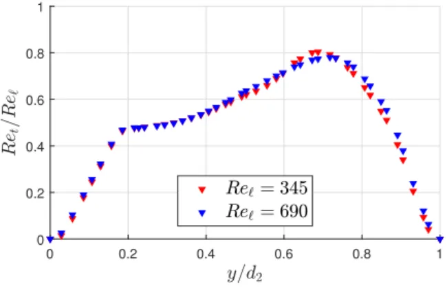
The profiles of Ret/Re`are plotted along the line 3 and presented in Fig.10. They are almost identical, even though Ret/Re`for Re`=345 is slightly larger than for Re`=690 in the mainstream region (y/d2=0.62 0.8). However, as expected, close to the walls, the ratio decreases to 0 as Retis zero at the walls.
0 0.2 0.4 0.6 0.8 1 0 0.2 0.4 0.6 0.8 1
Figure 10. Ratio of turbulence Reynolds number Retto Reynolds number Re`along the line 3 for the RSM model in 3D.
Therefore, the turbulence Reynolds number Rethas the same order of magnitude as the global Reynolds number Re`. A detailed analysis of the terms constituting this ratio allows to understand this finding :
Ret Re` = k e k |u|2inlet |u|inlet dinlet . (21)
The ratio k/e is a time scale (noted tL). This time scale is larger at the inlet than inside the baffles because the flow is almost laminar at the inlet Ret⇠ 0, Fig.9. In addition, this time scale is also relatively larger in the vortex zone than in the mainstream flow. The smaller the mixing time is, the more agitated and turbulent the flow is. The time scale increases when the Reynolds number decreases. The term |u|inlet
dinlet has the magnitude order of 10 3[s 1], while |u|2k inlet has the magnitude order of 1 and k/e is in the order of 103[ms] (see Fig.11).
The ratio k/e is presented in Fig.11for Re`=345 and Re`=690 for the RSM model in 3D. It is important to compare the values of k/e in the vortex region to the characteristic time of clay particles tk. In general, the clay particles diameter is in the order of dp=2 200 [µm]. Mean clay density is about rp=1700 [kg.m 3]. When replacing these values in the equation:
tp=d2p18µrp (22)
we find thattp=0.37 ⇥ 10 3 3.7 [ms]. Whereas the sedimentation velocity is equal to:
Ug=d2p(r18µp r)g (23)
where g is the acceleration due to gravity [m.s 2], and d
pis the diameter of the particle [m]. We find Ug=1.5 ⇥ 10 6 1.5 ⇥ 10 2[m.s 1]. Therefore, the dripper clogging is rather related to the flow hydrodynamics, low velocity and low turbulence kinetic energy k, as obtained at the inlet section and in the first vortex zone, which is also noticed by the works of Ait-Mouheb et al. (2019 [1]), and Yu et al. (2017 [37]) . Inside the labyrinth-channel unit, the larger k/e, the larger the mixing time occurs in the vortex zone center. This value is associated with the lower velocity magnitude which plays an important role in the capture of particles. However, the vortex center is less influential if
0 15 30 45 60 75 90 0 2.5 5 7.5 10 12.5 15 17.5 20 (a) Re`=345 0 7.5 15 22.5 30 37.5 45 0 1.25 2.5 3.75 5 6.25 7.5 8.75 10 (b) Re`=690
Figure 11. Ratio k/e, [ms] for RSM model in 3D.
the particles diameter is small and thustpis very small (Yu et al., 2017 [37]). Indeed, dripper clogging is worse when the physical particles are not isolated and accompanied by other causes of clogging such as the formation of biofilm (Gamri et al., 2015 [13]).
4. Vortex detection and analysis
The study of the flow velocity shows that the flow inside the baffles is composed of a mainstream flow and a vortex zone. This vortex zone was first observed when considering the streamlines of velocity fields (Fig.4). In order to identify swirling and shearing motion zones, a specific analysis is performed in this section to define with more accuracy these two zones.
4.1. Strain rate and vorticity
The deformation rate of the fluid is an important property. The deformation tensor describes how fluid elements deform as a result of fluid motion. This deformation (or velocity gradient) tensor is represented by Di j=Oui, j(where O is the nabla operator) and defined by :
Di j=Oui, j=∂x∂ui j = 0 B B B B @ ∂u
∂x ∂u∂y ∂u∂z ∂v ∂x ∂v∂y ∂v∂z ∂w ∂x ∂w∂y ∂w∂z 1 C C C C A . (24)
As this is a second order tensor it can be decomposed into a symmetric and an anti-symmetric part. Applying this to the Jacobian matrix J = (—u)T, with symmetric and anti-symmetric components, S andW respectively, Di j=Si j+Wi j:
S =1 2 Ou +OuT = 1 2 0 B B B B B B @
2∂u∂x ∂u∂y+∂v∂x ∂u∂z+∂w∂x ∂v
∂x+∂u∂y 2∂v∂y ∂v∂z+∂w∂y ∂w ∂x+∂u∂z ∂w∂y+∂v∂z 2∂w∂z 1 C C C C C C A ; (25) W = 1 2 Ou OuT = 1 2 0 B B B B B B @
0 ∂u∂y ∂v∂x ∂u∂z ∂w∂x ∂v
∂x ∂u∂y 0 ∂v∂z ∂w∂y
∂w ∂x ∂u∂z ∂w∂y ∂v∂z 0 1 C C C C C C A . (26)
The diagonal components of the strain rate tensor S (∂u∂x,∂v∂y and∂w∂z) are the extensional strain rates. Note that ∂u∂x>0 for an elongating body and∂u∂x<0 for a shortening body. The strain rate due to shearing in the x-y plane is defined in the components of the strain rate tensor as:
Sxy=12✓ ∂u∂y+∂v∂x ◆
. (27)
Vorticity !w is a vector field defined as the curl (rotational) of the flow velocity !u vector. Its definition can be expressed by:
!w = O⇥!u . (28)
Therefore :
wz=∂v∂x ∂u∂y . (29)
The mean strain rate Sxyand vorticitywzare calculated from Eq.27and Eq.29(with the variables u and v replaced by u and v). Then, they are normalized by (|u|inlet/dinlet)for both Reynolds numbers for the third baffle in both the Micro-PIV experiments and the RSM modeling. For experimental data, the second-order centred difference scheme is used to calculate the derivatives. This scheme is chosen according to the study by Foucaut and Stanislas (2002) [11] which concludes that a second-order centred difference scheme is the most efficient way to obtain good accuracy of the derivatives. Fig.12shows an example of the quadratical mesh used to treat Micro-PIV data by a Matlab code. The velocity derivatives are therefore computed as:
∂vi ∂x = 1 2Dx(vi+1 vi 1) (30) ∂uj ∂y = 1 2Dy uj+1 uj 1 (31)
whereDx = Dxi=Dxi+1=Dxi 1 andDy = Dyi=Dyi+1=Dyi 1since all the cells are square for experimental data with spatial resolution of 34.4 ⇥ 34.4µm.
i-1, j+1 i-1, j i , j i, j+1 i+1, j i+1, j+1 i, j-1 i-1, j-1 i+1, j-1 xi xi+1 xi-1 yj yj+1 yj-1
Figure 12. A quadrilateral mesh used in micro-PIV treatment by Matlab code extracted from Mishriky and Walsh (2017) [29]. One can conclude (Fig.13to Fig.16)1that the mean strain rate as well as the mean vorticity values are not much
influenced by the Reynolds number when comparing the normalized fields for these two Reynolds numbers. The numerical results are rather close to those obtained experimentally. The observed results have a difference of about 10% along the line 3, except in the zones y/d2=0.35 0.55 and y/d2=0.55 0.65 on which a gap of 47% and 150% is observed forwzand Sxyrespectively. The last huge value is due to the fact that the sign of Sxyis changed over this zone (y/d2= 0.55 - 0.65) experimentally when numerically it keeps positive values. wzhas a large value for the flow in the separation zone (red zone, Fig.15), with a positive value for the bottom tooth and a negative value for the top tooth. Regarding the same zone in the fields of mean strain rate, one finds that the strain rate is also maximum in this zone. As a result of this, the mean vorticity could be used directly to identify vortices. But a problem associated with this method is that vorticity cannot distinguish between swirling motions and shearing motions (Kida et al., 1998 [22]). In addition, contrary to what is usually found for vortex zones, the normalized mean vorticity values in these zones are close to zero, as the variation of mean velocity occurs over a quite long distance (from y/d2=0 to y/d2=0.55, Fig.5).
(a) Re`=345 (b) Re`=690
Figure 13. Normalized mean strain rate fields Sxy/(|u|inlet/dinlet), Micro-PIV.
1As the field of view is = 2.2 mm ⇥ 2.2 mm for dp=1[µm], it is difficult to visualize an entire baffle. This is why the baffle is presented by
juxtaposition of two fields of view. The deviated results, at y=1.5 mm, are due to the line which separates these two fields. 17
-9 -8.5 -8 -7.5 -7 -6.5 2.5 2 1.5 1 0.5 0 -6 -4 -2 0 2 4 6 (a) Re`=345 -9 -8.5 -8 -7.5 -7 -6.5 2.5 2 1.5 1 0.5 0 -6 -4 -2 0 2 4 6 (b) Re`=690
Figure 14. Normalized mean strain rate fields Sxy/(|u|inlet/dinlet), RSM model.
(a) Re`=345 (b) Re`=690
Figure 15. Normalized mean vorticity fieldswz/(|u|inlet/dinlet), Micro-PIV.
-9 -8.5 -8 -7.5 -7 -6.5 2.5 2 1.5 1 0.5 0 -20 -10 0 10 20 (a) Re`=345 -9 -8.5 -8 -7.5 -7 -6.5 2.5 2 1.5 1 0.5 0 -20 -10 0 10 20 (b) Re`=690
Figure 16. Normalized mean vorticity fieldswz/(|u|inlet/dinlet), RSM model. 4.2. Advanced criteria
4.2.1. Definitions
In order to be more quantitative, the numerical and experimental data must be analyzed by advanced methods. There are several methods to identify coherent turbulent structures (eddies) in a quantitative way. There is so far no universal accepted method to identify a coherent structure (Haller, 2005 [17]; Green et al., 2007 [16]). Many of these
methods involve the mean velocity gradient tensor (Chakraborty et al., 2005 [8]; Green et al., 2007 [16]).
The characteristic equation is the equation which is solved to find matrix eigenvaluesl, also called the characteristic polynomial. For a general matrix Z, the characteristic equation in variablel is defined by det(Z lI) = 0. The characteristic equation for the tensor—u is then given by:
l3+Pl2+Ql + R = 0 , (32)
where P, Q and R are the three invariants of the mean velocity gradient tensor. l2-criterion. A symmetric tensor A is defined as follows:
A = S2+W2 . (33)
A is considered to determine if there is a local pressure minimum that entails a vortex. A vortex is defined as ”a connected region with two negative eigenvalues of A” (Jeong and Hussain, 1995 [19]). Since A is symmetric, it has real eigenvalues only. Thus, its two eigenvalues (l1andl2) are also real for a two-dimensional flow, and by ordering the eigenvaluesl1 l2 l3 the definition becomes equivalent to requiring thatl2<0. The local minimum of l2corresponds to a vortex core. If the value ofl2is positive, the shear motion only exists and the vortex motion disappears in the local flow field. This is called the Lambda-2 (l2) vortex criterion.
Q-criterion. One other commonly mentioned method is the Q-criterion (Green et al., 2007 [16]), where Q is defined as:
Q =1
2 kWk2 kSk2 ; (34)
The Q-criterion defines a vortex as a ” connected fluid region with a positive second invariant of—u ”. Coherent eddies are then defined as regions of the flow with positive values of Q and lower pressure than the immediate surroundings (Chakraborty et al., 2005 [8]), these can easily be visualized as isosurfaces. Looking at the definition of the second invariant, we can see that Q represents the local balance between shear strain rate and vorticity magnitude, defining vortices as areas where the vorticity magnitude is greater than the magnitude of rate-of-strain (Hunt et al., 1988 [18], V`aclav Kol`ar, 2007 [23]).
Eq.34is developed to implement the parameter Q in Fluent software and to process it under Matlab for Micro-PIV experiments. Q can be written, in 2D and 3D, as follows:
Q = 1 2 ✓∂u ∂x ◆2 +✓ ∂v∂y ◆2! ✓∂u ∂y ∂v ∂x ◆ in 2D ; (35) and Q = 1 2 ✓∂u ∂x ◆2 +✓ ∂v∂y ◆2 +✓ ∂w∂z ◆2! ✓∂u ∂y ∂v ∂x+ ∂u ∂z ∂w ∂x + ∂v ∂z ∂w ∂y ◆ in 3D . (36) 19
4.2.2. Criterion treatment
l2 criterion results are plotted on Fig.17and Fig.18for Micro-PIV and RSM respectively. The vortex center, for whichl2is the smallest (in magnitude) of negative sign, is defined with accuracy by this method. The colored-blue area represents the vortices in these figures. As observed for vorticity fields, thel2criterion underlines that the separation zone (just behind the baffle tooth) is the region with vortex cores.
(a) Re`=345 (b) Re`=690
Figure 17. Normalizedl2criterion, Micro-PIV.
-9 -8.5 -8 -7.5 -7 -6.5 2.5 2 1.5 1 0.5 0 -6 -4.25 -2.5 -0.75 1 107 (a) Re`=345 -9 -8.5 -8 -7.5 -7 -6.5 2.5 2 1.5 1 0.5 0 -6 -4.25 -2.5 -0.75 1 107 (b) Re`=690
Figure 18. Normalizedl2criterion, RSM model in 3D.
The Q-criterion identifies the cores of turbulent structures (Chakraborty et al., 2005 [8]) while thel2-criterion is a somewhat looser criterion than the Q-criterion but guarantees local pressure minima within the 2D plane (Dubief and Delcayre, 2000 [10]; Chakraborty et al. 2005 [8]). The drawback of the Eulerian methods is that they are not independent from the reference frame, i.e. they are not objective. As Green et al. (2007 [16]) also point out, this method requires the user to effectively choose the thresholds discretionally (as Q > 0 may be changed to a higher value for instance in order to visualize more easily the vortex).
(a) Shear motion zone (b) Vortex zone
Figure 19. Normalized Q criterion -Mean rate of strain (Q > 0) and vorticity (Q < 0) regions- for Re`=345, Micro-PIV.
(a) Shear motion zone (b) Vortex zone
Figure 20. Normalized Q criterion -Mean rate of strain (Q > 0) and vorticity (Q < 0) regions- for Re`=690, Micro-PIV.
The experimental Q-criterion fields obtained with Eq.35are plotted in Fig.19and in Fig.20for the lower and larger Reynolds numbers respectively. The Q-criterion fields obtained likewise with Eq.35are plotted in Fig.21and Fig.22
for the RSM model. The Q-criterion helps to separate and distinguish between the vortex zone and the shear motion zone. It appears that intensities vary linearly with the Reynolds number, while the size and position of the vortex zone vary very slightly with Re`. The Q-criterion confirms what is found by thel2criterion: the size and position of the region near the baffle teeth and that in which vortex occurs depend very little on the Reynolds number in the range of Reynolds numbers studied. Nevertheless, the limitations of these vortex zones are somewhat inaccurate since the Q values are very low. Therefore, the ratio of Q in 3D to Q in 2D is calculated numerically. This ratio allows determining with high accuracy the vortex regions. The Q-criterion is calculated in 2D and in 3D on the 3D geometry by Eq.35and Eq.36respectively. The fields presented in Fig.21and Fig.22are for the 3D equation. In Fig.23, the ratio of Q3D/Q2D is calculated and shown. This figure points out the limitations of the vortex zone where small positive values in 3D become small negative values in 2D when the third component is eliminated (as with Micro-PIV data).
-9 -8.5 -8 -7.5 -7 -6.5 2.5 2 1.5 1 0.5 0 -6 -5 -4 -3 -2 -1 0 107
(a) Shear motion zone
-9 -8.5 -8 -7.5 -7 -6.5 2.5 2 1.5 1 0.5 0 0 0.5 1 1.5 2 2.5 107 (b) Vortex zone
Figure 21. Normalized Q criterion -Mean rate of strain (Q > 0) and vorticity (Q < 0) regions- for Re`=345, RSM model in 3D.
-9 -8.5 -8 -7.5 -7 -6.5 2.5 2 1.5 1 0.5 0 -6 -5 -4 -3 -2 -1 0 107
(a) Shear motion zone
-9 -8.5 -8 -7.5 -7 -6.5 2.5 2 1.5 1 0.5 0 0 0.5 1 1.5 2 2.5 107 (b) Vortex zone
Figure 22. Normalized Q criterion -Mean rate of strain (Q > 0) and vorticity (Q < 0) regions- for Re`=690, RSM model in 3D.
5. Conclusion
The present paper analyzes the flow in a baffle-fitted labyrinth-channel constituting irrigation drippers thanks to Micro-PIV and RSM modeling. The detection and the characterization of the vortex zone in a milli-labyrinth-channel are presented and detailed in this paper. The main conclusions are as follows:
-9 -8.5 -8 -7.5 -7 -6.5 2.5 2 1.5 1 0.5 0 -2 -1 0 1 2 (a) Re`=345 -9 -8.5 -8 -7.5 -7 -6.5 2.5 2 1.5 1 0.5 0 -2 -1 0 1 2 (b) Re`=690 Figure 23. Q3D
• The ratio k/e can be used as variable to estimate the time delay between the two laser pulses within a pair since it determines the mixing time. This time is short in the vortex zone and long at the inlet.
• Advanced methods, the Q and l criteria, which serve to detect the vorticity and to deeper analyze the vortex zones, were implemented. Q andl2methods show that the vortex intensity is largest in the separation zone where the large vorticity values result from the change of flow direction. The vorticity values are larger in this zone than in the vortex region where vorticity remains rather weak. The Q criterion allows to distinguish between the shear motion and vortex zones. As a conclusion, just downstream the baffle, there is, as expected, a vortex region but of weak intensity in comparison with the mainstream flow, where the strong vorticity value is generated by the flow direction change.
• The RSM model, globally, can be considered as a reliable model to predict and characterize the flow in the labyrinth-channel. The results obtained by RSM model are in good agreement with the experimental results, a difference about of 5% in the mean velocity prediction, in the mainstream flow. The size and the position of vortex zone are similar to the experimental results. However, a difference gap of about 75% is observed in the estimation of the mean velocity.
These experimental results will be compared with 2D-3C Micro-PIV measurements from future work, on the same prototype with additional Reynolds number values. Data issuing from such experiments would allow to confirm the present numerical results concerning the third velocity component. Next, detecting the vortex zones, which are the main responsible of clogging problems in drip irrigation systems, and analyzing them in a quantitative way, in function of the third direction, is one of the main objectives of future work based on Micro-PIV data. Finally, these analyses and results will be used as a basis for studying two-phase flow by injecting particles. Moreover, having a precise and comprehensive aspect on the clogging topology and formation mechanism is essential to optimize an anti-clogging dripper.
Acknowledgements
This work has been funded by the seventh Framework Programme FP7-KBBE-2012-6:Water4Crops and the Aleppo University in partnership with the laboratories IRSTEA (Institut national de Recherche en Sciences et Tech-nologies pour l’Environnement et l’Agriculture) and IRPHE (Institut de Recherche sur les Ph´enom`enes Hors Equili-bre). The authors are grateful to Jean-Jacques Lasserre from Dantec Dynamics company.
References
[1] Ait-Mouheb, N., Schillings, J., Al-Muhammad, J., Bendoula, R., Tomas, S., Amielh, M., Anselmet, F., (2019) Impact of hydrodynamics on clay particle deposition and biofilm development in a labyrinth-channel dripper. Irrigation Science. 37(1): 1–10.
[2] Al-Muhammad, J. (2016) Flow in millimetric-channel: numerical and experimental study. PhD thesis, IRSTEA/Ecole Centrale Marseille, pp: 240.
[3] Al-Muhammad, J., Tomas, S., Anselmet, F. (2016) Modeling a weak turbulent flow in a narrow and wavy channel: case of micro-irrigation. Irrigation Science. 34(5): 361-377.
[4] Al-Muhammad, J., Tomas, S., Ait-Mouheb, N., Amielh, M., Anselmet, F. (2018) Micro-PIV characterization of the flow in a milli-labyrinth-channel used in drip irrigation. Experiments in Fluids. 59:181.
[5] Anderson, w., Bonhus, D. L. (1994) An Implicit Upwind Algorithm for Computing Turbulent Flows on Unstructured Grids. Computers Fluids. 23(1):1-21.
[6] Berkowitz, S. J. (2001) Hydraulic performance of subsurface wastewater drip systems. In on-site wastewater treatment. Proceedings of the Ninth National Symposium on Individual and Small Community Sewage Systems, The Radisson Plaza. (11-14 March 2001, Fort Worth, Texas, USA, Texas), ed. K. Mancl.,St. Joseph, Mich. ASAE 701P0009. pp. 583-592.
[7] Capretto, L., Cheng, W., Hill, M., Zhang, X. (2011) Micromixing Within Microfluidic Devices. Topics in Current Chemistry. 304 27–68. [8] Chakraborty, P., Balachandar, S., Adrian, R. J. (2005) On the relationships between local vortex identification schemes. Journal of Fluid
Mechanics. 535:189-214.
[9] Chou, P. Y. (1945) On velocity correlations and the solutions of the equations of turbulent fluctuation. Quarterly of Applied Mathematics. 3(1):38–54.
[10] Dubief, Y., Delcayre, F. (2000) On coherent-vortex identification in turbulence. Journal of Turbulence. 1:1-22.
[11] Foucaut, J. M., Stanislas, M. (2002) Some considerations on the accuracy and frequency response of some derivative filters applied to PIV vector fields. Measurement Science and Technology, IOP Publishing,13 (7):1058-1071.
[12] Fu, S., Launder, B. E., Leschziner, M. A. (1987) Modelling strongly swirling recirculating jet flow with Reynolds-stress transport closures. In sixth symposium on Turbulent Shear Flows, Toulouse, France.
[13] Gamri, S., Tomas, S., Khemira, M., Ait-Mouheb, N., Molle, B. (2015) Biofilm growth at high COD and particle concentration levels: application to the case of micro-irrigation emitters used for wastewater reuse. International Commission on Irrigation and Drainage. 26th Euro-mediterranean Regional Conference and Workshops, 12-15 October 2015, Montpellier, France.
[14] Gibson, M. M., Launder, B. E. (1978) Ground effects on pressure fluctuations in the atmospheric boundary layer. Journal of Fluid Mechanics. 86:491–511.
[15] Goldberg, D., Gornat, B., Rimon, D. (1976). Drip irrigation: Principles, design, and agricultural practices. Drip Irrigation Scientific Publica-tions.
[16] Green, M.A., Rowley, C. W., Haller, G. (2007) Detection of Lagrangian coherent structures in three-dimensional turbulence. Journal of Fluid Mechanics. 572: 111-120.
[17] Haller, G. (2005) An objective definition of a vortex. Journal of Fluid Mechanics. 525:1-26.
[18] Hunt, J. C. R., Wray, A. A., Moin, P. (1988) Eddies, stream, and convergence zones in turbulent flows. Center for Turbulence Research. Report CTR-S88:193-208.
[19] Jeong, J., Hussain, F. (1995) On the identification of a vortex. Journal of Fluid Mechanics. 285:69-94.
[20] Karmeli, D. (1977) Classification and flow regime analysis of drippers. Journal of Agricultural Engineering Research. 22: 165-173. [21] K¨ahler, C. J., Scholz, U., Ortmanns, J. (2006) Wall-shear-stress and near wall turbulence measurements up to single pixel resolution by means
of long-distance micro-PIV. Exp. Fluids 41:327–341.
[22] Kida S., Miura, H. (1998) Identification and Analysis of Vortical Structures. Eur. J. Mech. B/Fluids. 17(4): 471-488.
[23] Kol`ar, V. (2007) Vortex identification: New requirements and limitations. International Journal of Heat and Fluid Flow. 28:638-652. [24] Launder, B. E. (1989) Second-moment closure and its use in modelling turbulent industrial flows. International Journal for Numerical Methods
in Fluids. 9(6):963-985.
[25] Launder, B.E., Reece, W., Rodi. (1975) Progress in the development of Reynolds-stress turbulence closure. Journal of Fluid Mechanics. 68:537-566.
[26] Lee, J.H., Kevin, Monty, J. P., Hutchins, N. (2016) Validating under-resolved turbulence intensities for PIV experiments in canonical wall-bounded turbulent. Exp in Fluids 57: 129.
[27] Li, Y., Yang, P., Xu, T., Ren, S., Lin, X., Wei, R., Wu, H. (2008) CFD and digital particle tracking to assess flow characteristics in the labyrinth flow path of a drip irrigation emitter. Irrigation Science. 26: 427-438.
[28] Lien, F. S., Leschziner, M. A. (1994) Assessment of turbulence-transport models including non-linear RNG eddy-viscosity formulation and second-moment closure for flow over a backward-facing step. Computers and Fluids. 23(8):983-1004.
[29] Mishriky, F., Walsh, P. (2017) Towards understanding the influence of gradient reconstruction methods on unstructured flow simulations. Transactions of the Canadian Society for Mechanical Engineering. 41(2): 169-179.
[30] Palau Salvador, G., Arviza Valverde, J., Bralts, V. F. (2004) Hydraulic flow behavior through an in-line emitter labyrinth using CFD tech-niques. ASAE/CSAE Annual International Meeting. Paper Number: 042252 Ottawa, Ontario, Canada.
[31] Pitts, D., Haman, D., Smajstra, A. (1990) Causes and prevention of emitter plugging in micro-irrigation systems, Florida Cooperative Exten-sion Service Bulletin, vol 258. University of Florida, Florida.
[32] Pope, S. B. (2000) Turbulent flows. Cambridge University Press.
[33] Prasad, A. K., Adrian, R. J., Landreth, C. C., Offutt, P. W. (1992) Effect of resolution on the speed and accuracy of particle image velocimetry interrogation. Experiments in Fluids. 13(2):105-116.
[34] Wei, Z., Cao, M., Liu, X., Tang, Y., Lu, B. (2012) Flow behaviour analysis and experimental investigation for emitter micro-channels. Chinese Journal of Mechanical Engineering. 25: 729-737.
[35] Westerweel, J. (2000) Theoretical analysis of the measurement precision in particle image velocimetry. Exp Fluids 29:S3–12 [36] Westerweel, J. (2008) On velocity gradients in PIV interrogation. Exp Fluids. 44:831–842.
[37] Yu, L., Li, N., Lo. DOI 10.1007/s00348-007-0439-3ng, J., Liu, X., Yang, Q. (2018) The mechanism of emitter clogging analyzed by CFD–DEM simulation and PTV experiment. Advances in Mechanical Engineering. 10(1):1–10https://doi.org/10.1177/1687814017743025. [38] Zhang, J., Zhao, W., Wei, Z., Tang, Y., Lu, B. (2007) Numerical investigation of the clogging mechanism in labyrinth channel of the emitter.
International Journal for Numerical Methods in Engineering. 70: 1598-1612.


![Figure 12. A quadrilateral mesh used in micro-PIV treatment by Matlab code extracted from Mishriky and Walsh (2017) [29].](https://thumb-eu.123doks.com/thumbv2/123doknet/13757204.438097/18.892.356.532.229.377/figure-quadrilateral-micro-treatment-matlab-extracted-mishriky-walsh.webp)


