Acquisition and reconstruction techniques for improving rapid magnetic resonance imaging with applications in fetal imaging

Acquisition and Reconstruction Techniques for

Improving Rapid Magnetic Resonance Imaging with

Applications in Fetal Imaging ARCHIVES

MASSAC INSTITUTE

by

Yamin I. Arefeen

_{JUN 13 2019}

B.S., Rice University (2017)

LIBRARIES

Submitted to the Department of Electrical Engineering and Computer

Science

in partial fulfillment of the requirements for the degree of

Master of Science in Electrical Engineering and Computer Science

at the

MASSACHUSETTS INSTITUTE OF TECHNOLOGY

June 2019

@

Massachusetts Institute of Technology 2019. All rights reserved.

Signature redacted

A u th or ... ...

Department of Electrical Engineering and Computer Science

May 8, 2019

Certified

by...

Signature redacted

...

Elfar Adalsteinsson

Professor, Department of Electrical Engineering and Computer Science

Professor, Institute for Medical Engineering and Science

Signature redacted

Thesis Supervisor

A ccepted by ...

...

'

L )

_{Leslie A. Kolodziejski}

Professor, Department of Electrical Engineering and Computer Science

Chair, Department Committee on Graduate Thesis

Acquisition and Reconstruction Techniques for Improving

Rapid Magnetic Resonance Imaging with Applications in

Fetal Imaging

by

Yamin I. Arefeen

Submitted to the Department of Electrical Engineering and Computer Science on May 8, 2019, in partial fulfillment of the

requirements for the degree of

Master of Science in Electrical Engineering and Computer Science

Abstract

Magnetic Resonance Imaging (MRI) serves as a powerful and noninvasive medical imaging modality. It gives clinicians the ability to image a wide variety of physical parameters, control image content, and acquire images at arbitrary spatial orienta-tions and resoluorienta-tions. Recently, MRI has gained traction as a method to supplement the diagnostic capability of Ultrasound for pregnant mothers and fetuses. In par-ticular, MR images dominated by T2 contrast, an intrinsic tissue parameter, give

informative visualization for diagnosis.

Traditional T2 weighted imaging techniques take on the order of seconds to min-utes to acquire an image. However, due to the frequency and unpredictability of fetal motion, imaging techniques in fetal MRI must acquire a 2D image in under a sec-ond. T2-weighted fetal MRI techniques, called single shot acquisitions, achieve rapid imaging speed by acquiring all desired data after a single radio frequency excitation, but constraining all measurements to be taken after a single excitation produces im-ages with spatially dependent blurring and poor contrast. As a result, many single shot techniques produce images with reduced diagnostic capability, in comparison to methods with longer acquisition times.

This thesis aims to improve the diagnostic quality of T2-weighted single shot im-ages. We incorporate the physical effects of rapid imaging into the image acquisition model and solve the resulting underdetermined system of equations using prior knowl-edge. We verify the efficacy of the techniques both in simulation and invivo adult brain experiments. Finally, we discuss how our proof of concent technique and results can be translated to the fetal imaging context.

Thesis Supervisor: Elfar Adalsteinsson

Title: Professor, Department of Electrical Engineering and Computer Science Professor, Institute for Medical Engineering and Science

Acknowledgments

Elfar, thank you for being such a kind, supportive, and astute advisor, and giving me the opportunity to perform MRI research, even though I had no background in the subject. I have learned so much about the nature of research, how to choose problems, and how to colloborate with others under your guidance.

Jacob, your intellectual curiosity, willingness to engage with all of the finer tech-nical challenges of a problem, and desire to help your students is astounding. I am incredibly grateful for your guidance.

Borjan, thank you for all of the help and incredible patience with respect to data collection and sequence development for this project.

Kawin, thank you for first introducing shuffling to me and providing support for the experimental acquisitions.

Sid, thank you for your friendship and all of the technical help throughout the project.

Daniel, Congyu, and Berkin, thank you for all of your technical advice and help with scanning.

Nick, Irene, Sayeri, Junshen, Georgy, Ilias, and Jose, thank you for the providing a wonderful lab enviornment.

Megumi, thank you for all of your help, organization, and assistance.

Patrick, thank you for your friendship and the stimulating discussions over morn-ings and lunch.

Mia, I am so thankful that we moved to Boston at the same time. Your friendship has been an invaluable and joyful part of my life here.

Luke, Brian, Jen, Dor, Sidd, Vibhaa, Jess, Pritpal, Nalini, thank you for your friendship and helping me feel at home in Boston.

Blake, Phil, Jorge, Daniel, Aayan, Houston will always be home, in part, due to our friendship.

Ma and Baba, I owe everything to you. Thank you for the never ending support and love.

Contents

1 Introduction

2 Background, Related Work, and Problem Statement 2.1 The M RI Signal ...

2.2 Signal Equation and Fourier Interpretation of MRI 2.3 Image Contrast and the Ideal T2 Weighted Image 2.4 HASTE Acquisition . . . . 2.5 Related W ork . . . . 2.6 Problem Statement . . . . 3 Single-Sho 3.1 Theory 3.1.1 3.1.2 3.1.3 3.1.4 3.2 Metho 3.2.1 3.2.2 3.2.3 3.2.4 3.3 Results 3.3.1 L T2-shuffling 27 97

Incorporating Signal Decay into the HASTE Acquisition Model 27

Low Dimensional Representation of Signal Evolutions . . . . . 28

Incoherent Phase Encode Sampling . . . . 30

Regularization and the Inverse Problem . . . . 32

Is . . . . 3 3 Low Dimensional Basis Generation . . . . 33

Generating the Sampling Mask . . . . 34

Simulated Data . . . . 34 Invivo D ata . . . . 36 . . . . 3 7 Simulation Results . . . . 37 13 16 . . . . 16 . . . . 18 . . . . 20 . . . . 22 . . . . 23 . . . . 24

3.3.2 Invivo Results . . . . 38

3.4 D iscussion . . . . 43

4 Two Iteration Single Shot T2-shuffling with Dictionary Matching 44 4.1 T heory . . . . 44

4.1.1 Solving the Original Single Shot Shuffling Problem . . . . 45

4.1.2 Dictionary Matching for T2 Estimation and Voxel Binning . . 46

4.1.3 Basis for each Bin . . . . 46

4.1.4 Altering the Shuffling Acquisition Model . . . . 48

4.1.5 Sampling Pattern, Regularization, and the Inverse Problem . . 48

4.2 Reconstruction Implementation . . . . 49

4.2.1 Original T2 Shuffling Reconstruction Implementation . . . . . 49

4.2.2 Second Iteration Shuffling Reconstruction Implementation . . 51

4.3 M ethods . . . . 53

4.3.1 Basis Generation, Sampling Pattern, Simulated Data, and In-vivo D ata . . . . 53

4.4 R esults . . . . 54

4.4.1 Invivo Results . . . . 57

4.5 D iscussion . . . . 59

5 Conclusions and Future Work 61 5.1 Future Work . . . . 61

List of Figures

2-1 In the presence of an external BO, magnetization will align along the z

direction in equilibrium . . . . 17 2-2 After a 90*excitation pulse, the equilibrium magnetization tips

com-pletely onto the transverse plane. A 180'pulse tips the magnetization onto the negative z axis. . . . . 18 2-3 After a 90*excitation, the transverse component of the magnetization

decays and the longitudinal portion of the magnetization recovers, ac-cording to the intrinsic tissue properties T2 and TI respectively. . . . 19 2-4 Schematic representation of signal decay from two tissues, tissue A and

tissue B, where tissue A has a larger T2 value than tissue B. A spin echo image at TEl implies that the contrast between tissues A and B in the image will be dominated by difference in the two tissues signal am plitude at TEl. . . . . 20 2-5 Schematic representation of the spin echo imaging process. A 90*and

180'pulse are played, followed by the measurement of a phase encode point. During the wait, magnetization resets. Waiting for magneti-zation recovery results in imaging times on the order of seconds or minutes, making SE imaging infeasible for many applications, such as fetal M R I . . . . 21 2-6 Rather than acquiring all lines at the same echo time, HASTE acquires

all desired phase encode points after a single excitation. This implies that HASTE samples phase encode point at different echo times along the signal decay curves of the anatomy. . . . . 22

2-7 Images generated from simulated HASTE and Spin Echo acquisitions. Notice how HASTE exhibits spatially dependent blurring and ringing not present in Spin Echo images. . . . . 23 2-8 Visual depiction of incorporating signal decay into the acquisition model.

S applies the coil sensitivity operators, F applies the forward fourier transform, and M indicates when particular phase encode points are acquired in time. In order to more faithfully represent a single shot acquisition, one can model the time series of spatially dependent signal evolutions as the unknowns in the single shot acquisition model. . . . 25

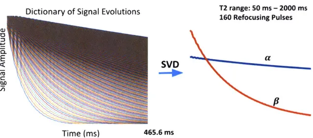
3-1 A typical dictionary of signal evolutions with T2 values between 50 and 2000 ms for a HASTE sequence with 465.5 ms acquisition time and 160'refocusing pulses. Concatenating the entries of the dictionary into columns of a matrix and taking a singular value decomposition yields two singular vectors that minimize dictionary characterization

in the Frobenius norm sense. . . . . 29 3-2 Some linear combination of the left two singular vectors can produce

signal evolutions associated with the HASTE sequence for different T2 values. Note, here we show the absolute value of the two singular vectors, and schematically represent their linear combination, rather

than showing the exact decay curves they produce. . . . . 30 3-3 The full T2 shuffling acquisition model. The spatially dependent

sig-nal evolutions are represented by two coefficient images. Passing the coefficient images through the low dimensional subspace, (D yields the spatially dependent signal evolutions, analagous to 7. The result is then multiplied by coil sensitivity maps and fourier transformed. The final masking operator identifies which phase encode points have been sampled during the echo train. By representing -y in a low dimensional subspace, one can vastly reduce the dimensionality of the problem de-scribed in 3.2. . . . . 31

3-4 The point spread functions induced by a shuffled sampling pattern versus a linear sampling pattern along a single readout line. Notice how a randomized sampling pattern spreads the aliasing incoherently between the two images. On the other hand, a linear sampling pattern induces a much larger, structured form of aliasing between the two images. This implies that a randomized sampling pattern produces a much better posed inverse problem to solve for the coefficient images. 32 3-5 The error of two basis vectors in representing signal evolution as a

function of T2 value in the dictionary. Notice how two basis vectors struggle to capture signal evolution assoiated with low T2 values. . . 34 3-6 (a) Sampling pattern indicating which phase encode point has been

sampled at each echo time for the simulation experiment. (b) Sampling pattern indicating which phase encode point has been sampled at each time for the invivo experiment. Notice how only a single phase encode point can be acquired at each echo time, due to the nature of a single shot acquisition. . . . . 35 3-7 (a) T2 map, (b) TI map, (c) proton density map, and (d) coil

sensi-tivity maps used in the simulation experiment. . . . . 35 3-8 (a) Sampling mask used to generate the oversampled result. Notice

the larger density of sampling in comparison to single shot shuffling. (b) Ability of three basis vectors to capture the range of T2 values. The oversampled reconstruction will provide a ground truth to which we will compare the invivo shuffling and HASTE images. . . . . 38 3-9 Simulated spin echo (ground truth), HASTE (baseline), and

synthe-sized shuffling images (ours) at echo times of TE = 75, 125, and 175 ms. Notice how the shuffling technique reduces upon the blurring and par-tial fourier artifacts present in the HASTE image, as indicated by the zoomed in view. However, the shuffling reconstruction, particularly at TE = 75 ms, exhibits contrast issues not present in the HASTE image, as indicated by the yellow arrow. . . . . 39

3-10 Error maps between the ground truth images to the HASTE (baseline) images and shuffling (ours) at TE = 75, 125, and 175 ms. In this viewpoint, the signal modulation issue becomes even more apparent, as shuffling seems to struggle with appropriate contrast in the low T2 value areas, particularly at TE = 75 ms. However, the shuffling error maps do not exhibit the same ringing or blurring artifacts present in the HASTE im ages. . . . . 40 3-11 Oversampled shuffling coefficients versus the single shot shuffling

coeffi-cients. The inversion resolves the coefficients with root-mean-squared-error of 18.3% compared to the oversampled reconstruction. Notice how the first coefficient seems well resolved, while some residual arti-facts remain in the second coefficient. . . . . 41 3-12 Oversampled shuffling reconstruction (target), synthesized single shot

shuffling images (ours), and HASTE reconstruction (baseline) at the three echo times of 83, 139, and 194 ms. Like in the simulation case, the shuffling reconstruction reduces blurring and partial fourier artifacts, as indicated by the zoomed in portions of the figure. Again, it seems like slight contrast issues persist particularly in low T2 values, as indicated by the yellow arrow. . . . . 42 3-13 Decay curves reconstructed by oversampled and single-shot shot

shuf-fling at a couple of select voxels. Single-shot shufshuf-fling poorly represents decay curves corresponding to lower T2 values. . . . . 43

4-1 (a) After solving the first iteration single-shot shuffling problem, recon-struct a decay curve at each voxel using the coefficients. (b) Estimate a T2 value at each voxel by dictionary matching the estimated decay curve to the dictionary of signal evolutions. (c) Group voxels into two bins based on T2 value, and construct a new basis for each bin which will be used to characterize voxels in that bin. In effect, each basis now covers a smaller dynamic range of signal evolutions, allowing for more accurate m odeling. . . . . 47 4-2 Error in capturing the dictionary of signal evolutions using a single

basis compared to multiple basis. Two bins with an individual basis for each bin much better characterizes the dictionary of signal evolutions, in comparison a single basis. . . . . 48 4-3 The point spread functions comparing a linear and shuffled sampling

pattern for the second iteration shuffling acquisition model. Notice how a shuffled sampling pattern induces lower magnitude, incoherent alias-ing between the coefficients. Randomly orderalias-ing phase encode points better poses both the first iteration and second iteration shuffling in-version . . . . . 50 4-4 Spin-Echo (ground truth), Shuffling (ours), Refined Subspace Shuffling

(ours), and HASTE (baseline) at three echo times. Both shuffling reconstructions reduce T2 blurring artifacts seen in HASTE. Notice how the second iteration of shuffling maintains more faithful spin echo contrast, in comparison to regular shuffling, particularly in the TE = 75 m s case. . . . . 55

4-5 Absolute error maps (x2) in comparison to a spin echo image at three echo times for the 1 mm resolution reconstructions. Root-mean-squared-error is computed with respect to the spin echo ground truth at the respective echo times. Regular shuffling (ours) and two iteration ba-sis refined shuffling (ours) both reduce image blurring, in comparison to HASTE (baseline). However, the two iteration version of shuffling maintains more faithful contrast in comparison to the spin echo image. Note, the original images are scaled between

[0,1]

it-eration shuffling coefficients and the corresponding error map. The in-version resolves the coefficients with root-mean-squared-error of 18.3% compared to the oversampled reconstruction. Qualitatively, it seems like the algorithm resolves the first coefficient accurately, while main-taining some residual artifacts in the second. . . . . 57 4-7 Images synthesized from the oversampled shuffling (target) method

versus HASTE images (baseline) and synthesized single shot shuffling (ours) and second iteration shuffling (ours) images at echo times of TE = 89, 139, 194 ms. Notice how the shuffling images reduce blurring and partial fourier artifacts in comparison to HASTE, as indicated by the zoomed in portions. Additionally, second iteration shuffling maintains more faithful signal contrast, in comparison to single shot suffling, as indicated by the yellow arrows. All images in the figure have been multiplied by 2 for the sake of visibility . . . . 58

4-8 RMSE map of how well single shot shuffling and second iteration re-solve decay curves at each voxel, in comparison to the oversampled shuffling decay curves. In particular, for each voxel in the image, we compute the decay curve produced by single shot shuffling, second iteration shuffling, and oversampled shuffling. We then compute the rmse of these two reconstructed decay curves in comparison to the over

sampled decay cuve for each voxel in the image. . . . . 59 5-1 Synthesized first iteration shuffling image (ours) versus corresponding

HASTE (baseline) and turbo spin echo (ground truth) images at TE = 75 ms. Although some residual artifacts remain, the shuffling image produces a sharper image than HASTE, as illustrated by the zoomed in view . . . . . 62

Chapter 1

Introduction

Magnetic Resonance Imaging (MRI) serves as a powerful, unique, and noninvasive medical imaging modality. Clinicians can image a wide variety of physical parameters and control image content through the manipulation of spins in atoms with odd numbers of protons or neutrons with magnetic fields [26]. Additionally, one can acquire images at arbitrary spatial orientations and resolutions. Due to its flexibility, MR can produce a wide variety of images on a range of anatomy: structural images with excellent soft tissue contrast, spectroscopy images, angiographic images, and time resolved images among many others [26].

Recently, fetal MRI has gained traction as a method to supplement the diagnostic capability of Ultrasound. With MRI, radiologists can diagnose abnormalities such as:

" Central nervous system disorders [11, 13, 19, 12, 31].

" Abdominal, pulmonary, and musculoskeletal concerns [13].

" Evaluation of maternal organs critical for fetal development, such as the pla-centa and cervix [13].

" Intracranial haemorrhage and ischaemic brain injury [311.

Radiologists detect many of the above abnormalities using T2- Weighted images, which serve as an excellent tool for diagnosis of abnormalities in fetal organs (brain,

lung, abdomen, urinary tract) and musculoskeletal and craniofacial structures [13]. In MRI, signal from different parts of the body decay at different rates, according to an intrinsic tissue property called T2. Differing T2 values of the anatomy in an image dominates the contrast in a T2-weighted image.

Due to the frequency and unpredictability of fetal motion, T2 weighted images must be acquired rapidly. Traditional techniques such as Turbo Spin echo (TSE) or Spin Echo (SE) take seconds or minutes to acquire an image; too slow for fetal MRI. Popular T2 weighted imaging techniques for fetal MRI, such as Half Fourier Single Shot T2 weighted acquisition (HASTE) or Single Shot Fast Spin Echo (SSFSE), acquire a 2D image in under a second [11, 30, 27]. However, single shot techniques exhibit spatially dependent blurring, poor contrast, and reduced diagnostic quality, in comparison to the slower TSE or SE methods [11].

In this thesis, we aim to improve single shot T2 weighted image quality in com-parison to traditional HASTE images. To do this, we first incorporate the physical effects of single shot techniques into the imaging acquisition model, resulting in an underdetermined system of equations. We resolve this underdetermined system of equations using the principles of incoherent random temporal sampling and low di-mensional subspace modeling recently described in a volumetric acquisition called T2-shuffling

[34].

Chapter 2 presents an introduction to the MR signal, the Fourier interpretation of MRI, ideal T2 weighted contrast generation, the HASTE sequence, related work, and the final problem statement. Chapter 3 will provide a more detailed explanation of T2 shuffling in a single shot context. Simulation and invivo results will be shown to illustrate the feasibility of single shot T2-shuffling, the benefits of applying the T2 shuffling framework, and the reason something beyond vanilla shuffling must be done to appropriately model signal evolution in the single shot regime. Chapter 4 will describe a second iteration refined subspace version of T2 shuffling. Again, simulation

and invivo results will be shown to illustrate the feasibility of this method and its improvement in signal evolution modeling. Finally, Chapter 5 will discuss how our proof of concent technique and results can be translated to the fetal imaging context. The work in this thesis served as the basis of the proposal which recieved an NSF Graduate Fellowship grant and was accepted as a digital poster presentation at the 27th annual meeting of the International Society for Magnetic Resonance in Medicine

(ISMRM)

* Yamin Arefeen, Nick Arango, Siddharth Iyer, Borjan Gagoski, Kawin Setsom-pop, Jacob White, Elfar Adalsteinsson. Refined-subspaces for two iteration single shot T₂-Shuffling using dictionary matching. International Society for Magnetic Resonance in Medecine 2 7th Scientific Meeting, Montreal,2019.

Chapter 2

Background, Related Work, and

Problem Statement

2.1

The MRI Signal

For a more detailed overview of the material in sections 2.1 and 2.2 of this chapter, we refer the reader to Nishimura's wonderful introduction to MRI book [26].

In the absence of an external magnetic field, atomic spins in anatomy orient them-selves randomly and maintain a net magnetic moment of 0. However the application of an external magnetic field, usually on the order of 1.5 - 7 Tesla, called BO, induces two interesting phenomena.

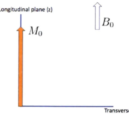
First, some of the atomic spins will align and produce a net magnetic moment in the direction of Bo, defined to be the z or longitudinal direction. In other words, one can imagine the net magnetic moment, Mo, to be oriented as a vector along the z-direction, as depicted by Figure 2-1.

Second, the spins will exhibit a resonance frequency defined by the Larmor Equa-tion,

W, =Bo (2.1)

Longitudinal plane (z)

M

Bo

Transverse Plane (xy)

Figure 2-1: In the presence of an external BO, magnetization will align along the z

direction in equilibrium.

will focus on structural imaging through the hydrogen atom. Radiofrequency fields, conventionally called B1, applied at a frequecy of w, in the tranverse direction (the

xy plane orthogonal to the z-direction) will excite the net magnetic moment out of equilibrium and tip some portion of the magnetization onto the transverse plane. For example, a 90'excitation will tip MO completely onto the transverse plane, while a 180'will tip Mo into the negative z-direction, as illustrated by Figure 2-2.

After B_{1 excitation, magnetization oriented along the transverse plane will begin} to precess at the larmor frequency. This precession induces the MRI signal as an electromotive force measured by a RF receive coil. Note, only the transverse portion of magnetization will precess and contribute to measured signal.

Following excitation, magnetization immediately will begin to recover along the longitudinal direction and decay along the transverse direction, governed by anatomy dependent time constants T1 and T2 respectively. In other words, magnetization

recovers back to its original equilibrium state, oriented along the z direction in the presence of BO. If we define MO, to be the equilibrium magnetization along the z-direction, magnetization recovery following a 90_{'excitation can be described as}

MZ(t) = MO(1 - eT) (2.2)

Longitudinal plane (z)

90I

Longitudinal plane (z)

Bo

Transvirse Plane (xy)

1800

n)

w

Bo

Transverse Plane (xy)

AI

Figure 2-2: After a 90*excitation pulse, the equilibrium magnetization tips completely onto the transverse plane. A 180*pulse tips the magnetization onto the negative z

axis.

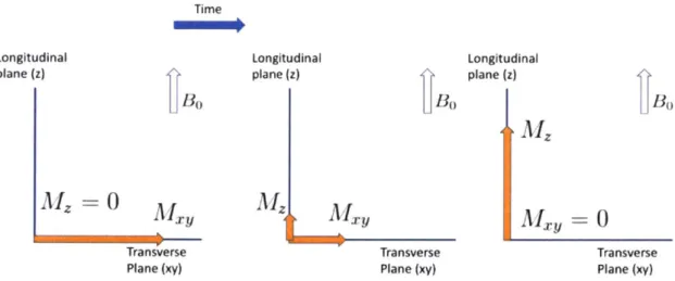
where Mz(t) and My(t) are longitudinal and transverse portions of magnetization respectively. Figure 2-3 visualizes the effects of relaxation following a 9 0_excitation.

2.2

Signal Equation and Fourier Interpretation of

MRI

After excitation, all spins tipped onto the transverse plane will precess at the larmor frequency. Linear magnetic fields then encode spatial position by inducing spins at different spatial locations to precess at different frequencies. In other words, the gradients induce a linear mapping between spatial position and frequency. Ignoring the effects of T1 and T2 relaxation for now, one can formalize the acquired MRI signal as,

Time

Longitudinal Longitudinal Longitudinal

plane (z) plane (z)

f

Bo Bo BA

AII

M

--

0

MyK,0

]VIZ= 0 INI VIIX AIXMAIX _{= 0}

Transverse Transverse Transverse

Plane (xy) Plane (xy) Plane (xy)

Figure 2-3: After a 90_{'excitation, the transverse component of the magnetization}

decays and the longitudinal portion of the magnetization recovers, according to the intrinsic tissue properties T2 and T1 respectively.

s(t) =

j

s(t) = Mxy (kx(t), ky (t)) + w(t) (2.4) Thus, MRI measures samples of the Fourier Transform, so called k-space in MR convention, based on the application of linear spatial encoding gradients. After dis-cretization, the acquisition can be modeled as linear operators,

y = Fx + w _(2.5)

where y E _{CN are measured k-space samples, x E CN is our desired image,}

F

C

c

2.3

Image Contrast and the Ideal T2 Weighted

Im-age

Although ignored in the previous section, after a 90'excitation, magnetization along the transverse plane evolves over time, due to relaxation. This evolution depends on the T2 and TI values at a particular spatial location and the RF pulses played after the initial excitation pulse.

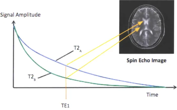
Contrast in a T2 weighted image corresponds to the signal intensity difference of different tissues at a particular imaging time, denoted echo time or TE, due to T2 decay. Figure 2-4 gives a schematic representation of T2 signal decay and of contrast in a T2 weighted image at a, particular echo time.

Signal Amplitude

j

T2

Spin Echo Image

T2

Time

TEi

Figure 2-4: Schematic representation of signal decay from two tissues, tissue A and tissue B, where tissue A has a larger T2 value than tissue B. A spin echo image at TEl implies that the contrast between tissues A and B in the image will be dominated by difference in the two tissues signal amplitude at TE1.

Spin echo imaging acquires a high fidelity T2 weighted images at a particular echo time

[3].

1. The scanner excites signal from the body using a 90_{'excitation pulse.}

2. In practice, system imperfections result in signal decay much faster than a tissue's T2 value. Therefore, the scanner plays a 180*RF pulse to refocus the MR signal such that the signal achieves the value governed by T2 decay at the desired TE.

3. The ADC samples a line of k-space, also called a phase encode point, at the desired TE.

4. The scanner pauses for magnetization to relax back to equilibrium. 5. Steps 1-4 are repeated until all all phase encode points are acquired.

Figure 2-5 gives a schematic representation of the SE imaging process. Although SE imaging produces high signal-to-noise-ratio (SNR) and sharp T2 weighted images, acquisitions can take on the order of seconds to minutes.

Refocusing ADC

-**

I

4

Figure 2-5: Schematic representation of the spin echo imaging process. 180'pulse are played, followed by the measurement of a phase encode poi

A 90'and nt. During the wait, magnetization resets. Waiting for magnetization recovery results in imaging times on the order of seconds or minutes, making SE imaging infeasible for many applications, such as fetal MRI

Excitation 901,

Reset -*Wait

2.4

HASTE Acquisition

HASTE, the predominant T2 weighted imaging technique in fetal MRI, accelerates imaging time by acquiring all desired phase encode points after a single 90'excitation. The MR community refers to these methods as single shot techniques. In particular, after the initial 90'excitation, the scanner implements an alternating train of ADC read outs and 180'refocusing pulses to sample phase encode points and ensure that signal exhibits relaxation as closely as possible to T2 decay at each readout line. Unlike a SE acquisition, HASTE acquires all phase encode points at different echo times after excitation, as illustrated by Figure 2-6. By convention, the time at which HASTE samples the center line of k-space is denoted to he nominal TE of a HASTE acquisition. Fourier Transform Ky _{Signal Amplitude} Line 1 Line 2 Line 3 _T2 Kx -Line 16( TE 160 T2 Time

Unes acquired TE1 TE2 TE3

at different TE's

Figure 2-6: Rather than acquiring all lines at the same echo time, HASTE acquires all desired phase encode points after a single excitation. This implies that HASTE samples phase encode point at different echo times along the signal decay curves of the anatomy.

The naive HASTE acquisition model can be written as,

.4

where y E CN is our acquired data, x c CN is our desired HASTE image, F is the

2D DFT operator, and M is the undersampling mask indicating which phase encode points have been sampled.

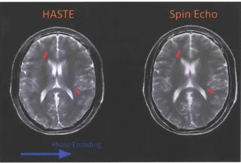
HASTE will produce a T2 weighted image. However, notice how the acquisition model does not incorporate information about signal evolution. In particular, the model implicitly assumes that all phase encode points have been sampled at the same echo time. This mismatch between model assumption and reality produces spatially dependent blurring in the final reconstructed HASTE image. Figure 2-7 illustrates the exaggerated effect of spatially dependent blurring by comparing a simulated HASTE image to a simulated SE image.

HASTE

Spin Echo

Figure 2-7: Images generated from simulated HASTE and Spin Echo acquisitions. Notice how HASTE exhibits spatially dependent blurring and ringing not present in Spin Echo images.

2.5

Related Work

Many MR methods have been proposed to mitigate the effects of signal evolution during acquisition.

Some methods estimate signal evolution and then post process the MR measure-ment 140, 28, 10]. However, these techniques are sensitive to the signal evolution

estimate and have not been extended to single shot techniques.

Other methods utilize a low dimensional subspace to model signal decay, and then pose a linear acquisition model to solve for a time series of images along the signal decay curve [39, 17, 18]. These methods have not been extended to the single shot regime and estimate T2 parameter maps, which we do not aim to do.

T2-shuffling exploits the forward model of signal evolution to reconstruct multiple, sharp images along the signal decay curve [34, 1, 33]. Like some of the aforementioned methods, shuffling relies on a low dimensional subspace to model signal decay in each voxel, but also introduces compressed sensing principles into the acquisition. Shuffling mitigates blurring and produces multiple images from a single scan. However, the technique utilizes multiple excitations to acquire 3D images, as opposed to acquiring 2D images with a single excitation.

One can also design the refocusing pulses to mitigate signal decay and reduce the amount of spatially dependent blurring [6, 22]. These techniques have been applied to the single shot regime, but they do not model signal evolution during the acquisition, and some level of blurring persists in the images.

Compressed sensing, parallel imaging, and deep learning methods have also been implemented to accelerate single shot T2 weighted acquisitions and reduce blur-ring [7, 8]. Rather than modeling signal decay, these techniques mitigate blurblur-ring by accelerating the acquisition and stabilizing signal with variable refocusing pulses.

2.6

Problem Statement

In this work, we aim to improve single shot T2 weighted image quality in comparison to traditional HASTE images by incorporating the effects of signal evolution into the acquisition model. Form the three dimensional object -y E CNxNxT which represents the signal evolution at each voxel in the image throughout the course of an acquisition. The single shot acquisition model can then be written as,

where S is the forward coil sensitivity operator, F is the 2D DFT, y c CNxNxCxT represents our acquired data, and M E CNxNxCxT is the sampling mask indicating which phase encode point is acquired at each echo time. Figure 2-8 gives a visual depiction of the acquisition model described above. Note, the figure was inspired by figures in [34].

Coils

E

Figure 2-8: Visual depiction of incorporating signal decay into the acquisition model. S applies the coil sensitivity operators, F applies the forward fourier transform, and M indicates when particular phase encode points are acquired in time. In order to more faithfully represent a single shot acquisition, one can model the time series of spatially dependent signal evolutions as the unknowns in the single shot acquisition model.

Due to the nature of single shot acquisitions, only T phase encode points can be acquired. By incorporating spatially dependent signal evolutions into the acquisition model, we are now in the presence of a highly underdetermined system of equations, as we need resolve -', which has N x N x T unknowns with only N x T measurements (corresponding to T acquired phase encode points).

The remainder of the thesis will discuss the techniques utilized to resolve the un-derdetermined system of equations described in Equation 2.7 and produce a sharp, time resolved series of images. In order to illustrate success, qualitative image com-parisons, error maps, and quantitative comparisons between a to be described ground truth, HASTE, and our proposed techniques will be reported for simulation experi-ments. For in-vivo experiments, qualitative image comparisons will be shown

Chapter 3

Single-Shot T2-shuffling

We begin by revisiting the acquisition model described in Equation 2.7 that incorpo-rates signal evolution to model a single shot acquisition. This modeling yields a highly underdetermined system of equations, which we resolve utilizing the techniques of T2 shuffling. By doing this, we can solve for a time series of sharp T2 weighted images from a single HASTE-like acquisition. We demonstrate the ability of our technique to reduce signal blurring in simulation and invivo adult experiments. Finally, we discuss limitations in the modeling capability of T2 shuffling within the context of single shot imaging.

3.1

Theory

3.1.1 Incorporating Signal Decay into the HASTE Acquisition Model

The HASTE forward model can be written as,

y = MFSx (3.1)

where x

E

F is the forward fourier transform, M E RNxNxC is the sampling mask indicating sampled phase encode points, and y E CNxNxC is our acquired data. Notice, how the

acquisition model fails to incorporate signal decay and implicitly assumes all phase encode points have been sampled at the same echo time.

Assume that we acquire T phase encode points, which corresponds to T echoes, during a single shot acquisition. Form the three dimensional object -Y C CNxNxT

which represents the signal evolution at each voxel in the image during acquisition. The acquisition model can be modified as follows,

y = MFSy (3.2)

where S and F represent the forward coil sensitivity and fourier operators which operate along the first two spatial dimensions, M C CNxNxCxT is the sampling mask identifying which phase encode point has been sampled at each echo time, and y E CNxNxCxT is the new representation of our acquired data. Figure 2-8 gives a visual representation of the model described in Equation 3.2.

By incorporating spatially dependent signal evolutions into the acquisition model, we are now in the presence of a highly underdetermined system of equations, as we need to solve for N x N x T unknowns with N x T measurements. We turn to

core principles of T2-shuffling [34] in order to solve the system of equations: low dimensional representation of signal evolutions, incoherent temporal sampling, and sparse regularization.

3.1.2

Low Dimensional Representation of Signal Evolutions

A range of physiologically reasonable T2 values characterize signal evolution in a voxel during a HASTE acquisition. One can simulate a dictionary of signal evolutions by simulating a HASTE sequence for a set of T2 values that cover the range of physiologically reasonable values. Let X C CTxD be a dictionary of simulated signal evolutions. Let D C CTxT be some orthonormal basis such that

X = 4pHX (3.3)

Dictionary of Signal Evolutions T2 range: 50 ms - 2000 ms 160 Refocusing Pulses

SVD

Time (ms) 465.6 ms

Figure 3-1: A typical dictionary of signal evolutions with T2 values between 50 and 2000 ms for a HASTE sequence with 465.5 ms acquisition time and 160'refocusing pulses. Concatenating the entries of the dictionary into columns of a matrix and taking a singular value decomposition yields two singular vectors that minimize dic-tionary characterization in the Frobenius norm sense.

such that

X-<Dk<X X < (3.4)

for some tolerance c

[34].

[34]

k ~ <DH<Dfy (3.5)

a

_{a, .}

ba

Figure 3-2: Some linear combination of the left two singular vectors can produce signal evolutions associated with the HASTE sequence for different T2 values. Note, here we show the absolute value of the two singular vectors, and schematically represent their linear combination, rather than showing the exact decay curves they produce.

Defining a = @H7, we arrive at the T2 shuffling forward model,

y = MFS(Da (3.6)

where y, M, F, S, and 4% are as defined previously, and a C CNxNxk are k coeffi-cient images which represent how much each basis vector in Ik needs to be weighted by to produce the desired signal evolution in each voxel of the image. Although the system still remains underdetermined, low rank modeling vastly reduces the dimen-sionality of the problem as we now only have N x N x k unknowns where k

<<

3.1.3

Incoherent Phase Encode Sampling

Imposing a low rank prior on our unknown signal evolutions vastly reduces the di-mensionality of our unknowns, but the single shot T2 shuffling system still remains underdetermined. In order to resolve the system, we apply the idea of incoherent

tem-Coils

Figure 3-3: The full T2 shuffling acquisition model. The spatially dependent signal evolutions are represented by two coefficient images. Passing the coefficient images through the low dimensional subspace, (D k yields the spatially dependent signal evo-lutions, analagous to -y. The result is then multiplied by coil sensitivity maps and fourier transformed. The final masking operator identifies which phase encode points have been sampled during the echo train. By representing -y in a low dimensional subspace, one can vastly reduce the dimensionality of the problem described in 3.2. poral sampling introduced by T2 shuffling in the spirit of compressed sensing 123].

Rather than sampling phase encode points in linear order, as done in traditional HASTE, one can sample the phase encode points randomly throughout time to induce incoherent undersampling artifacts between the coefficients images.

Define 6_{k E CNxNxk to have a 1 in the center of the first coefficient and zeros}

everywhere else. The extent of coupling between the coefficients can be analyzed by passing 6k through the forward and adjoint shuffling operators to compute the

corresponding pointspread function for coefficient k [211,

PSFk = pHSH FHMFSbk6k. (3.7)

Figure 3-4 compares the point spread functions along the center readout line for a linear HASTE sampling pattern and a temporally shuffled sampling pattern for k = 2 coefficients (since we are phase encoding in one direction, the point spread function will be the same across all readout lines). Notice how the linear sampling pattern induces large structural aliasing between the two coefficients, while the randomized sampling pattern induces lower, incoherent aliasing between the two coefficients. This

Input Coefficient 1

Input Coefficient 2

Figure 3-4: The point spread functions induced by a shuffled sampling pattern versus a linear sampling pattern along a single readout line. Notice how a randomized sampling pattern spreads the aliasing incoherently between the two images. On the other hand, a linear sampling pattern induces a much larger, structured form of aliasing between the two images. This implies that a randomized sampling pattern produces a much better posed inverse problem to solve for the coefficient images. implies that a randomized sampling pattern produces a better posed inverse problem to solve for the coefficient images, a.

3.1.4

Regularization and the Inverse Problem

One can solve for the shuffling coefficients through a regularized-least squares inverse problem,

1

min, IMFS4ka - y 1 + Ag(a)

22 (3.8)

where g imposes some sort of prior on the coefficient images. The authors of the original T2 shuffling paper apply a locally low rank prior on patches of a

[381.

In this work, we apply a l1-regualirzed Wavelet prior to exploit sparsity in a

[23],

E

E

which yields the single-shot T2-shuffiing inverse problem,

1

min, IMFSDka - yl l+ AllWalli (3.9) 22

The inverse problem described above can be solved using first order proximal gradient methods such as FISTA [2].

3.2

Methods

3.2.1

Low Dimensional Basis Generation

We acquire 140 phase encode points for all simulated shuffling acquisitions and 80 phase encode points for all invivo shuffling acquisitions. To generate 4Dk, we first simulated a dictionary of signal evolutions, X, using 2000 evenly spaced T2 values beteen 50 and 2000 ms and a TI value of 1000 ms using the extended phase graph algorithm [16, 37], resulting in a dictionary with 2000 entries. We choose a T2 range between 50 and 2000 ms to capture signal evolution from tissues with white matter, gray matter, and CSF, and we choose just one T1 value due to the insensitivity of HASTE signal evolution to T1 [6, 5, 32, 36].

We then take the singular value decomposition of our dictionary,

X = UEVH (3.10)

and take the first k left singular vectors of U to be 1_{Dk. We empirically have found}

that we can solve for at most k = 2 coefficient images in the single shot regime. Figure 3-5 reports the representation error of 2 basis vectors in characterizing signal evolution in the dictionary as a function of T2. Notice how two basis vectors do a relatively poor job of representing signal evolutions corresponding to low T2 values.

45 %

-

Error

Single Basis

on

T2

value

Figure 3-5: The error of two basis vectors in representing signal evolution as a function of T2 value in the dictionary. Notice how two basis vectors struggle to capture signal evolution assoiated with low T2 values.

3.2.2

Generating the Sampling Mask

In order to produce an incoherent temporal sampling pattern, first define the set P to be the indices of the 24 center (auto calibration lines) phase encode points and the indices of the other phase encode points to be acquired. Then, uniformly randomly shuffle P to produce P. P denotes which phase encode point should be sampled at the i" echo time.

We utilized the first and second sampling patterns in Figure 3-6 for the simulation and invivo experiments respectively. Notice how only a single phase encode point can be sampled at each echo time, due to the nature of a single shot sequence.

3.2.3

Simulated Data

We obtained realistic T1, T2, and proton density brain maps with matrix size 256 x 256 and 1 mm in plane resolution from the Brainweb database [9]. Realistic coil sensitivity maps were also obtained, having been calibrated utilizing the ESPIRiT algorithm [35]. Figure 3-7 shows the aforementioned T1, T2, proton density, and coil sensitivity maps.

Figure 3-6: (a) Sampling pattern indicating which phase encode point has been sam-pled at each echo time for the simulation experiment. (b) Sampling pattern indicating which phase encode point has been sampled at each time for the invivo experiment. Notice how only a single phase encode point can be acquired at each echo time, due to the nature of a single shot acquisition.

Figure 3-7: (a) T2 map, (b) T1 map, (c) proton density map, and (d) coil sensitivity maps used in the simulation experiment.

Given these parameters maps, we utilized the EPG algorithm to simulate the signal evolution at each voxel during a HASTE acquisition. A 90'excitation pulse, 160'refocusing pulses, an echo spacing of 5 ms, and 140 echoes were used for simula-tion. Simulation produced -Ygt C CNxNxT which represents the ground truth signal

evolution at each voxel in the image given the simulated HASTE acquisition. We then generated our undersampling mask, Mim, using sampling pattern (a) illustrated in Figure 3-6. Finally, we produced the acquired data with,

ysjim = MsimFSygt (3.11)

HASTE acquisitions for comparison were also simulated by replacing Mim with a linear sampling pattern which sampled the DC phase encode point at TE = 75, 125, and 175 ms respectively. In order to achieve the appropriate echo time, the three simulated HASTE acquisitions measured 86, 96, and 106 phase encode points with 9/16, 10/16, and 11/16 partial fourier respectively.

The shuffling inverse problem was solved using FISTA with 100 iterations and a regularization parameter of A = 1 x 10-. The HASTE acquisitions were reconstructed using GRAPPA with projection onto convex sets partial fourier [14, 15].

3.2.4

Invivo Data

A healthy adult subject was scanned using the modified HASTE sequence described earlier on a 3T Siemens machine with a 32-channel head coil. For single shot T2-shuffling acquisitions, 5 slices were obtained with an echo spacing of 5.56 ms, voxel res-olution of 1.4 x 1.4 x 3 mm, field-of-view of 358.4 x 358.4 mm, 80 sampled phase encode points (corresponding to a 445 ms acquisition), 90*excitation pulse, and 160'refocusing pulses. The phase encode points were sampled in the random order illustrated by sampling pattern (b) in Figure 3-6.

HASTE images were also acquired for comparison. In order to replicate the shuf-fling acquisition as closely as possible, 5 slices were obtained with equivalent echo spacing, voxel resolution, FOV, excitation pulses, and refocusing pulses. Only the

number of phase encode points was varied such that we could acquire HASTE images with the center DC line sampled at TE - 83, 139, and 194 ms. In particular, we

acquired three different HASTE acquisitions with 86, 96, and 106 phase encode points and 9/16, 10/16, and 11/16 partial fourier to achieve the aforementioned echo times. Note, the voxel size, echo spacing, refocusing pulses, and echo times used in both the HASTE and shuffling acquisitions mimic the parameters in clinical fetal MRI.

Coil sensitivity maps were reconstructed from the HASTE data using a SURE-based automatic parameter selection version of ESPIRiT

120].

We solved the shuffling inverse problem using FISTA with 80 iterations and a regularization parameter of A = Ix 10-4. The HASTE acquisitions were reconstructed using GRAPPA with projection onto convex sets partial fourier.

Finally, we acquired multiple single-shot shuffling acquisitions so that we could perform a multi-shot T2 shuffling reconstruction in order to compare and quantify the performance of our single shot T2 shuffling reconstruction to a more densely sampled ground truth. We solved the multi-shot T2 shuffling inverse problem with setting

k = 3, using FISTA with 48 iterations, and applying locally low rank regularization

with A = 1 x 10-4. The sampling mask for this more densely sampled case and the ability of three basis vectors to capture the dictionary of signal evolutions can be seen in Figure 3-8.

3.3

Results

3.3.1

Simulation Results

Figure 3-9 shows simulated spin echo (ground truth), HASTE (baseline), and syn-thesized shuffling images (ours) at echo times of TE = 75, 125, and 175 ms. In the shuffling acquisitions, we synthesized spin-echo contrast through estimating T2 val-ues at each voxel with dictionary matching, and picking off the value on the resulting exponential decay curve for each voxel, based on the echo time. Notice how shuffling reduces the blurring present in HASTE, as indicated by the zoomed in views.

How-_________________________________________________________________ 4

b.

10%

2%

T2 Value (ms)

Figure 3-8: (a) Sampling mask used to generate the oversamlpled result. Notice the larger density of sampling in comparison to single shot shuffling. (b) Ability of three basis vectors to capture the range of T2 values. The oversampled reconstruction will provide a, ground truth to which we will comipare the invivo shuffling and HASTE images.

ever, the yellow arrows indicate region with low T2 value where shuffling synthesizes incorrect contrast, due to the inability of two basis vectors to appropriately capture signal evolution.

Figure 3-10 illustrates error maps between the spin echo images versus the HASTE and synthesized shuffling images TE -= 75, 125, and 175 ms. Note, the absolute error maps have been scaled between [0,I] and multiplied by 3 for visibility. In this viewpoint, the signal modulation issue becomes even more apparent, as shuffling does not appropriately represent contrast at low T2 values in comparison to HASTE. On the other hand, blurring and ringing error artifacts seem to be reduced in the shuffling images.

3.3.2 Invivo Results

Figure 3-11 illustrates the oversampled shuffling coefficients versus the single shot shuffling coefficients. The inversion resolves the coefficients with root- mean- squared-error of 18.3% compared to the oversampled reconstruction. Notice how the first

Figure 3-9: Simulated spin echo (ground truth), HASTE (baseline), and synthesized shuffling images (ours) at echo times of TE = 75, 125, and 175 ms. Notice how the shuffling technique reduces upon the blurring and partial fourier artifacts present in the HASTE image, as indicated by the zoomed in view. However, the shuffling reconstruction, particularly at TE = 75 is, exhibits contrast issues not present in the HASTE image, as indicated by the yellow arrow.

Figure 3-10: Error maps between the ground truth images to the HASTE (baseline) images and shuffling (ours) at TE = 75, 125, and 175 ms. In this viewpoint, the signal modulation issue becomes even more apparent, as shuffling seems to struggle with appropriate contrast in the low T2 value areas, particularly at TE = 75 ms. However, the shuffling error maps do not exhibit the same ringing or blurring artifacts present in the HASTE images.

Figure 3-11: Oversampled shuffling coefficients versus the single shot shuffling coeffi-cients. The inversion resolves the coefficients with root-mean-squared-error of 18.3% compared to the oversampled reconstruction. Notice how the first coefficient seems well resolved, while some residual artifacts remain in the second coefficient.

coefficient seems well resolved, while some residual artifacts remain in the second coefficient.

Figure 3-12 shows the oversampled shuffling reconstruction (target), synthesized single shot shuffling images (ours), and HASTE reconstruction (baseline) at the three echo times of 83, 139, and 194 ins. Like in the simulation case, the shuffling recon-struction reduces blurring and partial fourier artifacts, as indicated by the zoomed in portions of the figure. The yellow arrows indicate areas, corresponding to regions with low T2 values, with slight contrast issues in the shuffling images.

Figure 3-13 shows decay curves reconstructed by oversampled and single-shot shot shuffling at a couple of select voxels. Single-shot shuffling poorly represents decay curves corresponding to lower T2 values.

Figure 3-12: Oversampled shuffling reconstruction (target), synthesized single shot shuffling images (ours), and HASTE reconstruction (baseline) at the three echo times of 83, 139, and 194 ms. Like in the simulation case, the shuffling reconstruction reduces blurring and partial fourier artifacts, as indicated by the zoomed in portions of the figure. Again, it seems like slight contrast issues persist particularly in low T2 values, as indicated by the yellow arrow.

7a

1,

E

a

4,

Figure 3-13: Decay curves reconstructed by at a couple of select voxels. Single-shot corresponding to lower T2 values.

E

0

z

oversampled and single-shot shot shuffling shuffling poorly represents decay curves

3.4

Discussion

Signal decay during an echo train of 80 echoes (roughly 440 ns) often results in T2-weighted HASTE images with poor diagnostic quality. In this chapter, we modeled signal decay by incorporating it into the acquisition model, and solved the resulting underdetermined system of equations utilizing T2 shuffling. We have found, both in simulation and invivo, that shuffling can be used to reasonably reduce blurring and partial fourier artifacts. However, due to the inability of two basis vectors to capture a wide dynamic range of signal evolutions, single-shot shuffling can produce images with contrast not indicative of the synthesized echo time.

In the following section, we will introduce an alternative version of single-shot T2 shuffling which ainis to better capture signal evolutions for all T2 values using just two basis vectors per voxel.

Chapter 4

Two Iteration Single Shot T2-shuffling

with Dictionary Matching

In the previous chapter, we incorporated signal decay into the HASTE acquisition model, resulting in a highly underdetermined system of equations that we resolved utilizing the techniques of T2 shuffling. In particular, we imposed that signal evolution at each voxel can be well represented by two basis vectors. However, we found that two basis vectors do not capture the entire dynamic range of signal evolutions; as a result, the single-shot shuffling images exhibited some contrast issues.

In this chapter, we propose a two iteration version of T2 shuffling which better cap-tures signal evolution with just two basis vectors per voxel, while still reconstructing a time series of images with reduced blur and partial fourier artifacts, in comparison to HASTE.

4.1

Theory

We begin by providing a high level overview of the algorithm. The two-iteration version of T2 shuffling follows 4 main steps:

1. Solve the single-shot shuffling inverse problem to produce an estimated decay curve at each voxel in the image.