Comparison of data-driven analysis methods for identification of functional connectivity in fMRI

Comparison of Data-Driven Analysis Methods for

Identification of Functional Connectivity in fMRI

by

Yongwook Bryce Kim

Sc.B. Mathematics and Physics

Brown University, 2005

Submitted to the Department of Electrical Engineering and Computer

Science

in partial fulfillment of the requirements for the degree of

Master of Science in Electrical Engineering and Computer Science

at the

MASSACHUSETTS INSTITUTE OF TECHNOLOGY

February 2008

@

Massachusetts Institute of Technology 2008.

Author ...

All rights reserved.

- - - ' ... . ... ...W...

Department of Electrical Engineering and Computer Science

January 29, 2008

Certified by.

...

Polina Golland

Assistant Professor of Computer Science and Engineering

Thesis Supervisor

Accepted by ...

APR 0 7 2008

SLIBRARIES

/

Terry P. Orlando

Chairman, Department Committee on Graduate Students

Comparison of Data-Driven Analysis Methods for

Identification of Functional Connectivity in fMRI

by

Yongwook Bryce Kim

Submitted to the Department of Electrical Engineering and Computer Science on January 29, 2008, in partial fulfillment of the

requirements for the degree of

Master of Science in Electrical Engineering and Computer Science

Abstract

Data-driven analysis methods, such as independent component analysis (ICA) and clustering, have found a fruitful application in the analysis of functional magnetic reso-nance imaging (fMRI) data for identifying functionally connected brain networks. Un-like the traditional regression-based hypothesis-driven analysis methods, the principal advantage of data-driven methods is their applicability to experimental paradigms in the absence of a priori model of brain activity. Although ICA and clustering rely on very different assumptions on the underlying distributions, they produce surpris-ingly similar results for signals with large variation. The main goal of this thesis is to understand the factors that contribute to the differences in the identification of functional connectivity based on ICA and a more general version of clustering, Gaussian mixture model (GMM), and their relations. We provide a detailed emprical comparison of ICA and clustering based on GMM. We introduce a component-wise matching and comparison scheme of resulting ICA and GMM components based on their correlations. We apply this scheme to the synthetic fMRI data and investigate the influence of noise and length of time course on the performance of ICA and GMM, comparing with ground truth and with each other. For the real fMRI data, we pro-pose a method of choosing a threshold to determine which of resulting components are meaningful to compare using the cumulative distribution function of their em-pirical correlations. In addition, we present an alternate method to model selection for selecting the optimal total number of components for ICA and GMM using the task-related and contrast functions. For extracting task-related components, we find that GMM outperforms ICA when the total number of components are less then ten and the performance between ICA and GMM is almost identical for larger numbers of the total components. Furthermore, we observe that about a third of the components of each model are meaningful to be compared to the components of the other. Thesis Supervisor: Polina Golland

Acknowledgments

My time as a MIT student has been a challenging, but enjoyable one. There were many rough times, but I have grown up personally and intellectually from such ex-periences. I am grateful that I have had great opportunities to learn the importance of staying healthy, being open to differences, and being happy with myself in this stimulating environment. I can never thank enough the people around me at MIT whom I am greatly indebted.

First of all, I would like to express my sincere gratitude to my research advisor Professor Polina Golland for her unwavering support and encouragement, helping me stay focused, and teaching me how to think critically and carefully. I appreciate her enormous understanding and patience, especially regarding my health conditions. I will always remember her invaluable advice, openness, and passion. I'd also like to thank Professor John Gabrieli for the opportunity to work closely with his group in BCS and Professor Nancy Kanwisher for providing the data used in this thesis.

The members of the vision group have been always great to work with. Thanks to Ray and Thomas for helping my transition into the group. Thanks to Wanmei, Danial, and Sune for heated research discussions, listening to my ideas, and providing helpful feedbacks. I appreciate the members of the EECS KGSA for providing the home away from home. Thanks to Junghoon, Taegsang, and Sejoon for fruitful conversations. My special appreciation goes to Bo. Thanks for sharing with me your valuable time and dreams.

I thank the Boston Red Sox for providing me one of the greatest distractions. It was worth it, again.

And finally, as always, I am deeply grateful to my family for their endless encour-agement and love. Thanks mom and dad for unconditional support and trust. Thanks Yongjoo for being the best brother and life-time friend. We often find ourselves in different continents in the world, but you are always in my heart.

Contents

1 Introduction

2 Functional Magnetic Resonance Imaging

2.1 Overview ...

2.2 fMRI Experimental Protocols ... 2.3 Preprocessing ...

2.4 Signal-to-Noise Ratio of fMRI Signal ... 2.5 Summary ...

3 Functional Connectivity

3.1 Brain Connectivity ...

3.2 Standard Regression-based Hypothesis-driven Functional Connectivity . . . . 3.3 Prior W ork ...

3.4 Summary ...

4 Data-Driven Methods

4.1 Principal Component Analysis . . . . 4.2 Probabilistic Principal Component Analysis 4.3 Independent Component Analysis . . . .

4.3.1 Generative Model . . . . 4.3.2 Independence of Sources . . . . 4.3.3 The Infomax Algorithm . . . .

Method for Detecting

27 28 29 30 33 35 . . . . 36 . . . . 41 . . . . 44 . . . . 45 . . . . 46 . . . . 48

4.3.4 Maximum Likelihood Formulation ... 50

4.3.5 Spatial ICA for fMRI ... 51

4.4 Clustering: Gaussian Mixture Model ... ... .. 53

4.5 Model Selection ... ... ... 58

4.6 Sum m ary ... ... ... ... 60

5 Empirical Study 61 5.1 Comparison Scheme ... 61

5.1.1 Preprocessing and Component Selection ... 61

5.1.2 Comparison between ICA and GMM. ... 62

5.2 Synthetic Data ... 65

5.2.1 Data Generation ... 65

5.2.2 Effects of Noise on the Identified Components ... 68

5.2.3 Effect of the Length of Experiment on the Identified Components 72 5.3 Real fMRI Experiments ... 78

5.3.1 Description of Data ... 78

5.3.2 Comparison on Task-related Components ... 79

5.3.3 Component-wise Comparison between ICA and GMM ... 81

5.4 Sum m ary ... ... 90

6 Discussion and Conclusions 91

List of Figures

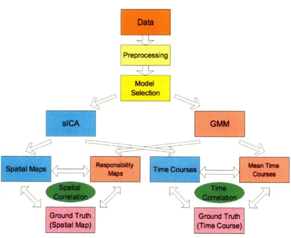
5-1 Comparison scheme of ICA, GMM, and the ground truth. The ground

truth is not available for real fMRI studies for components other than

the ones corresponding to the experimental protocol. ... . 63

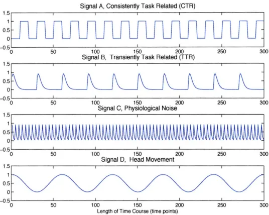
5-2 Synthetic Data Signals. Signal A is consistently task related with

block-design waveform. Signal B is generated as a gamma function to rep-resent transiently task related component. Signal C is also a gamma function modeeling physiological noise. Signal D is a sine wave

simu-lating head motion. ... 66

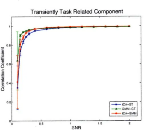
5-3 Component-wise comparison of the effect of noise level on the spatial correlation of the estimated sICA and GMM maps with ground truth and with each other. T = 300 time points. Error bars come from ten independent repeats. ... 70 5-4 Component-wise comparison of the effect of noise level on the time

correlation of the estimated sICA and GMM time courses with ground truth and with each other. T = 300 time points. Error bars come from ten independent repeats. ... ... 71

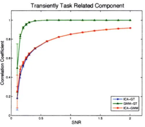
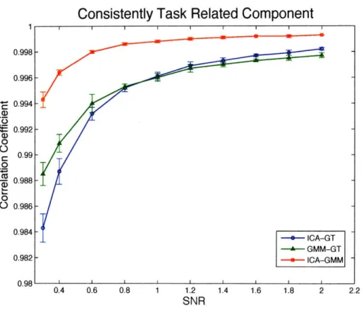
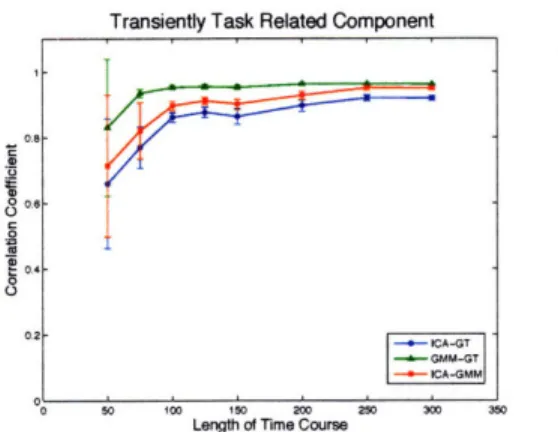
5-5 Zoomed plot of consistently task related component in time. Below

SNR = 1, GMM outperforms ICA. Above SNR = 1, ICA outperforms

GMM. Error bars come from ten independent repeats. ... . 73

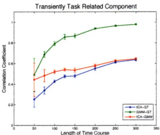
5-6 Component-wise comparison of the effect of length of time courses on the spatial correlation of the estimated sICA and GMM spatial maps with ground truth and with each other. SNR = 0.3. Error bars come from ten independent repeats. ... 75

5-7 Component-wise comparison of the effect of length of time courses on the time correlation of the estimated sICA and GMM time courses with ground truth and with each other. SNR = 0.3. Error bars come

from ten independent repeats. ... 76

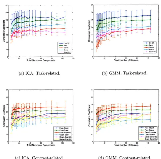
5-8 Comparison of the ground truth to the best matched ICA and GMM components in time for different total number of components. .... 80 5-9 Component-wise comparison of ICA and GMM with K = 15

compo-nents. ... 83

5-10 Component-wise comparison of ICA and GMM with K = 30

compo-nents. ... 86

5-11 Component-wise comparison of ICA and GMM with K = 50 components. 87 5-12 Component-wise comparison of ICA and GMM with K = 80 components. 88 5-13 Component-wise comparison of ICA and GMM with K = 105

List of Tables

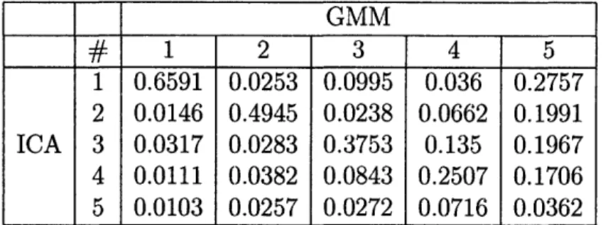
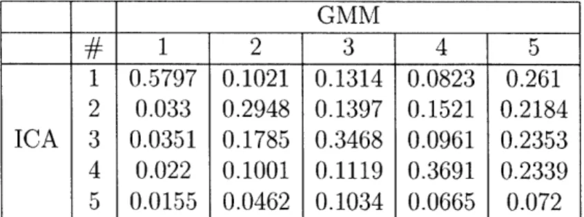
5.1 Average of the absolute values of correlations coefficient between ICA and GMM components for SNR = 0.1. ...

5.2 Average of the absolute values of correlations coefficient between ICA and GMM components for T = 50. ...

A.1 Average of sulting ICA A.2 Average of

sulting ICA

the absolute values of correlations coefficient between re-and GMM spatial maps for real fMRI study. K = 15.. the absolute values of correlations coefficient between

Chapter 1

Introduction

Since its development in the early 1990s, functional magnetic resonance imaging (fMRI) has played a tremendous role in visualizing human brain activity for the study of mechanisms of human brains and clinical practice. Acquired by a regular magnetic resonance machine with special parameter settings, this non-invasive imag-ing method measures changes in blood flow, which in turn are an indication of neural activity. fMRI produces four-dimensional time-series images (three-dimensional in space and one-dimensional in time) with relatively low temporal resolution and high spatial resolution.

This new imaging technique has generated a large volume of new high dimensional data and hence, the need for new image analysis methods. In the recent literature, in-teresting discoveries in human cognitive states have been found using techniques from machine learning, especially multivariate pattern analysis and non-linear pattern clas-sification methods [20, 34, 55]. Much of the work in fMRI data analysis has revolved around the detection of activation at different locations. In addition to localizing ac-tivity, we are also interested in how the "activated" areas are related and connected to each other. Functional connectivity, the central theme of this thesis, characterizes these functional interactions anmd coordinated activations among different parts of the brain.

Traditionally, the regression based, hypothesis-driven approach has been used to detect functional connectivity. Taking this approach, a "seed" region of interest must

be first selected by the user. The network is defined as the areas whose correlation with the seed time course exceeds a pre-defined threshold. This method can work well when the goal is to identify regions that co-activate with a certain part of the brain. Hypothesis-driven methods require prior information on the protocol and hypothesis of an experiment to model the expected hemodynamic response. Moreover, the correlation threshold, directly related to the statistical significance level, must be

selected.

Recently, there has been an increasing number of fMRI experiments that inves-tigate the brain activity in a more natural, near protocol-free setting, such as re-sponding to audio-visual input like a movie or rest state scanning [10, 11, 17, 30, 65]. Unlike traditional protocol-based experiments, these new complex experiments do not contain a well-defined onset protocol. Although the traditional seed-based connec-tivity analysis can be applied to these data, paradigm-free, data-driven exploratory methods such as principal component analysis (PCA) [26], independent component analysis (ICA) [49], and clustering algorithms [30, 32] such as Gaussian mixture model can naturally provide an alternative to comparing each voxel's time course against a hypothesis. They explore the data to find "interesting" components or underlying sources. Structures or patterns in the data, which are difficult to identify a priori, such as unexpected activation and connection, motion related artifacts, and drifts, may be revealed by these components. However, the direct relationship among the

data-driven methods is largely unknown and the performance in correctly detect-ing and classifydetect-ing functionally connected regions depends on various theoretical and experimental factors.

Recently, several works have compared data-driven analysis methods in the con-text of functional connectivity. Baumgartner et al. [6] use artificially generated acti-vations and show that fuzzy clustering analysis (FCA) outperforms principal

compo-nent analysis in a noisy data setting by comparing the maximum Pearson correlation coefficient between the simulated activation time course and the representative time courses obtained by FCA and PCA. The superior performance of ICA compared to

connec-tivity in the resting brain and the effect of seed selection on CCA results are presented in [47]. Meyer-Baese et al. [50] present comparative results of several variations of clustering and ICA algorithms by evaluating their performances using task-related activation maps and associated time courses with respect to the experimental proto-col in a simple block design fMRI experiment and by conducting receiver operating characteristic analysis. They show a close agreement between clustering and ICA, but also conclude that despite a longer processing time, clustering outperforms ICA in terms of the classification results of the task-related activation. Smolders et al. [58] compare results of fuzzy clustering and ICA in terms of within- and between-subject consistency and spatial and temporal correspondence of obtained maps and time courses. They demonstrate a good agreement between FCA and spatial ICA in discriminating the contribution of distinct networks of brain regions to the main cognitive stages of the task (auditory perception, mental imagery and behavioural response). They claim that whereas ICA works optimally on the original time series, averaging with respect to the task onset (and thus introducing some a priori infor-mation on the experimental protocol) is essential in the case of FCA leading to a richer decomposition of the spatio-temporal patterns of activation. However, for all of these studies, their comparison scheme was only based on the similarity of the task related component detected by the methods to a predefined reference waveform and disregarded all other components.

Exploratory data analysis methods have also been compared in other areas of medical image analysis and computer vision. Jung et al. [41] show the advantages of ICA over PCA in removing electroencephalographic (EEG) artifacts. In the context of face recognition, the literature on the subject is contradictory. Bartlett et al. [5], Liu and Wechsler [45] claim that ICA outperforms PCA for face recognition, while Baek et al. [3] report a contrary result that PCA outperforms ICA when tested on the FERET database. Delac et al. [21] and Draper et al. [23] conclude that the performance of methods (PCA, ICA, and Linear Discriminant Analysis) largely depends on a particular task of face recognition such as subject identification and expression recognition and that one method cannot be claimed to perform better

than others in general cases.

Although ICA and clustering rely on very different assumptions on the under-lying distributions, they produce surprisingly similar results for signals with large variation. The main goal of this thesis is to understand the factors that contribute to the differences in the identification of functional connectivity based on ICA and a more general version of clustering, Gaussian mixture model (GMM), and their re-lations. Using the synthetic data with artificial activations and artifacts generated by the generative model of ICA under two experimental conditions (length of the time course and signal-to-noise ratio (SNR) of the data), both spatial maps and their associated time courses estimated by ICA and GMM are compared to each other and to the ground truth. The number of components are chosen via the model se-lection scheme and all selected components are compared, not just the task-related components. This comparison scheme is verified in a real fMRI study.

This work provides a detailed comparison of ICA and clustering based on Gaussian mixture model, both in terms of generative models and experimental conditions. Contributions of this thesis are as follows.

* We devised a component-wise matching and comparison scheme of resulting ICA and GMM components using their correlations.

* We applied this scheme to the synthetic data and investigated the influence of noise and length of time course on the performance of ICA and GMM, compar-ing with ground truth and with each other.

* We developed a method of choosing a threshold to determine which of result-ing components are meanresult-ingful to compare usresult-ing the cumulative distribution function of their empirical correlations.

* We proposed an alternate method of selecting the optimal total number of components for ICA and GMM using the task-related and contrast functions. * We applied our methods to real fMRI data in visual recognition experiments.

With ever increasing volume of complex experimental fMRI data, we believe that our work will provide a better understanding of the functional brain networks and a direction for further analysis.

The rest of the thesis is organized as follows. In Chapter 2, we review the basic properties of fMRI, typical fMRI experiment set-ups, pre-processing steps, and the sources of noise in fMRI data. In Chapter 3, we compare three definition (anatomical, functional, effective) of brain connectivity. We also define and explain the notion of functional connectivity. In addition, we discuss previous work on this topic and the standard hypothesis-driven connectivity analysis method. In Chapter 4, we describe the generative models and the algorithms for the three data-driven connectivity mod-els of our interest, PCA, ICA, and GMM and model selection methods. Chapter 5

introduces the component-wise comparison scheme between ICA and GMM. Further-more, we present the results of investigating the differences of performance of the analysis methods using synthetic and real fMRJ data in Chapter 5. We conclude with discussion of future research directions in Chapter 6.

Chapter 2

Functional Magnetic Resonance

Imaging

2.1

Overview

Functional magnetic resonance imaging (fMRI) is a recently developed neuroimaging modality that provides an opportunity to study functional human brain activity in a non-invasive way. MRI uses strong magnetic fields to create images of biological tissue. To generate images, an MRI scanner applies a series of changing magnetic gradients and oscillating electromagnetic fields, known as a pulse sequence. By varying this pulse sequence, a particular tissue type of interest (e.g. gray and white matter, tumors, bone damage) can be detected by the scanner. Functional neuroimnaging aims to localize different mental processes to different parts of the brain, in effect creating a map of which areas are responsible for which processes. Since the early

1990s, the development of fMRI has catalyzed an explosion of interest in functional neuroimaging and has become a powerful tool in research and clinical applications.

Unlike structural MR1, which measures differences between tissues, fMRI nmea-sures signal changes in the brain that are due to changing neural activity. The most popular approach is the fMRI based on blood oxygenation level dependent. (BOLD) signal changes, which allows assessment of brain activity via local hemodynamic vari-ations over time [51, 64]. The basic assumption is that increased neural activity

induces an increased demand for oxygen and, in turn, the vascular system increases the amount of oxygenated hemoglobin relative to deoxygenated hemoglobin. Because deoxygenated hemoglobin attenuates the MR signal, which causes a change in the MR decay parameter T2, the vascular response leads to a signal increase that is re-lated to the neural activity. This process is known as hemodynamic response (HDR). In a typical fMRI experiment, external stimuli are presented at intervals of several seconds, causing a change in voxel-signal intensity, delayed and blurred by the hemo-dynamic response lag. From these changes, researchers can make inferences about the underlying neural activity and how different brain regions may participate in dif-ferent perceptual, motor, or cognitive processes. However, the precise nature of the relationship between neural activation and the BOLD signal is a subject of current research and is yet to be well understood. Because changes in blood oxygenation oc-cur intrinsically as part of normal brain physiology, fMRI is a non-invasive technique that can be repeated on the same subject as many times as needed.

fMRI provides one of the optimal combined spatial and temporal resolution meth-ods presently available for non-invasive functional brain mapping. Typically, it gen-erates voxels with a spatial resolution of 2 to 5 mm and a temporal resolution of few seconds. However, one of the main drawbacks of fMRI is the relatively low im-age signal-to-noise ratio (SNR), which is the magnitude of the signal change due to experimental condition divided by the variability in the measurements, depending on both the amount and variability of signal change. Along with other factors such as artifacts, head movement, and undesired physiological sources of variability, this makes detection of the activation-related signal changes a difficult task.

Despite its limitations, fMRI has been widely used in many different application domains in psychology, neurobiology, neurology, radiology, biomedical engineering, electrical engineering, physics, and many others. Especially in cognitive neuroscience, due to its adaptability to many types of experimental paradigms, fMR.I has shown great utility in researching object processing and recognition, memory, visual atten-tion, language plasticity, and connectivity between brain regions, to name a few. With a better understanding of the BOLD effect and hemodynamic response and more

so-phisticated data acquisition and analysis techniques, fMRI has a great potential to be used even more widely in research and clinical applications.

2.2 fMRI Experimental Protocols

To functionally associate one or more brain regions with a task that a subject per-forms, one must first devise an experimental design. Simple tasks in fMRI experi-ments include presentation of sounds and images, whereas more complex experiexperi-ments involve watching movies and presentation of instructions for memory and recognition tasks, for example. Experimental design is followed by the image acquisition step, in which the subject lies in a MRI scanner performing a task with his head fixed to avoid movement artifact. These acquired images are used to draw a cognitive inter-pretation via careful statistical analysis. The experimental design is commonly based on a block-design or an event-related design.

In the case of the block design, each condition is presented for an extended time period, and the different conditions are usually alternated over time. Typically, a block design involves alternations of a task-performing block and a rest block, where no stimuli are presented. A block, also referred as an epoch, contains a sequence of several repetitions of stimuli under the same condition. A single condition may include more than one cognitive task. Block design considers all of them as a single task condition. This is the case of our real visual recognition fMRI data, presented in Chapter 5. Due to the large amount of noise is present in fMRI data, the underlying signal, which should follow the periodic activation pattern, is hardly recognizable even when the voxel is taken from a strongly activated region. This low signal-to-noise ratio of fMRI makes detection of any activation difficult with only one realization of a condition. Thus, the fMRI algorithms are based on averaging over several realizations since averaging increases the signal-to-noise ratio. However, the limiting factor in multiple realizations of experimental conditions is the subject's ability to perform identical tasks without moving or getting tired, which introduces motion artifacts and fatigue effects.

An alternative to the block design is the event-related design, which involves a different stimulus structure. Although the block design has an advantage of excellent detection power, the event-related design has the ability to estimate the shape of the hemodynamic response function. Event-related designs present stimuli one at a time rather than together as a block. Such experimental protocols are characterized by rapid, randomized presentation of stimuli. Time between each trial of stimuli is typically jittered. This has the advantage that the subject does not get used to the experiment, which ensures that the HRF does not change its shape or decrease in amplitude. This is necessary to enable averaging over several realizations. Further-more, different trial types are intermixed so that each trial is statistically independent from other trials. Since it assumes that the HRFs corresponding to various tasks are different, signals can be analyzed by task category. The possibility of post hoc cat-egorization of an event is another advantage of event-related fMRI. It is in general difficult to draw a conclusion which type of experimental design is better. The design which best suits a specific research hypothesis should be chosen.

2.3

Preprocessing

Preprocessing includes all processes that are performed after image reconstruction and prior to the statistical analysis of the data. The two primary goals of preprocessing are to reduce non-task-related variability in experimental data and to improve validity of statistical analysis [36].

Since almost every fMRI scanner acquires the slices of a volume in succession, each slice is obtained at a different time point. Slice timing correction shifts each voxel's time series within a repetition time (TR) so that all voxels in a given volume appear to have been captured at exactly the same time. This is especially important for long TRs, in which the expected hemodynamic response amplitude can vary significantly. Slice timing correction is typically done using temporal interpolation, which uses information from nearby time points to estimate the amplitude of the signal at the onset of the TR. Interpolation strategies include linear, spline, and sinc interpolations.

Another very important preprocessing step is motion correction. fMRI analysis assumes that each voxel represents a unique part of the brain. In case of head motion, each voxel's time course could be acquired from more than one brain location. The effect of head motion on the signal change is significant, especially near the edge of the brain. A movement of one tenth of a voxel may produce 1-2% signal change, which is not negligible, compared to the very small amount of signal change of fXMRI BOLD effects [29]. This requires the use of accurate image registration algorithms to spatially align multiple image volumes. The images are transformed by resampling with respect to a reference image, which is often the first acquired image. In case of the rigid body transformation, the transformation parameters (translation, rotation) for the images are determined by optimizing the goodness of fit to the reference image

[28].

In order to facilitate comparisons of the results of analyses aross different subjects, the images in the data are normalized according to a template in the standardized space. This process is called spatial normalization. The most commonly adopted coordinate system is that described by Talairach and Tournoux [60]. Although spatial normalization allows generalization of results to larger population and provides a coordinate space for reporting results, matching between subjects is only possible on a coarse scale, since there is not necessarily a one-to-one mapping of the cortical structures between different brains. No such processing was required in our work, since we did not perform the analysis across subjects.

Spatial filtering with a Gaussian smoothing kernel is often applied to increase signal-to-noise ratio in the data. The increase in SNR is achieved by applying a filter which has the same shape and size as the signal. However, the effectiveness of spatial smoothing diminishes if exact signal properties are not known and the size of the smoothing kernel is larger than the activation area. In the temlporal domain, applying a high-pass filter suppresses slow, repetitive physiological signals related to the cardiac cycle or to breathing, as well as the scanner-related drifts.

In some studies, a region of interest (ROI) is selected through segmentation, which classifies voxels within an image into different anatomical divisions. It allows direct,

unbiased measurement of activity within an anatomical region, based on the assump-tion that funcassump-tional divisions tend to follow anatomical divisions.

2.4

Signal-to-Noise Ratio of fMRI Signal

Although fMRI has been shown useful and is used extensively in neuroscience research, the level of signal changes in fMRI data still remain low (approximately 1-2%). Signal-to-noise (SNR) ratio is one way to quantify the level of signal changes in the fMRI data. SNR is typically defined as the ratio of the variability in the signal to the variability in the noise. We define SNR in the General Linear Model framework [27], which models the brain as a linear time invariant system with an impulse response function reflecting the hemodynamic properties of the brain. We use design matrix B = [B1, B2] for linear regression. GLM assumes the signal is a linear combination of a protocol-dependent component, B1, a protocol-independent component, B2, such as physiological noise and drifting, and random noise, E. We construct B1 by convolving the experimental protocol and the assumed hemodynamic response function modelled as a two gamma function [39], defined as

h(t)

_di

l exp

_bi

-

_d2

exp

_b2

(2.1)

where dj = ajbj is the time to the peak and al = 6, a2 = 12, bl = b2 = 0.9s, and

c = 0.35. The two gamma function correctly captures the small dip after the HRF has returned to zero. Typically, low order polynomials are used to model B2. For a

given time course

p',

& = B131i + B232i + ±, (2.2)

where ,@ = [/01, 2i] is a vector of estimated amplitudes of the hemodynamic responses and the protocol independent signals at voxel i. Noise - - N(0, Ej). The noise covariance E• is unknown. Assuming the noise is white, Ej = oaI, we can estimate )

using the least square estimate,

= (BTB)-'BT . (2.3)

For a given voxel i, we define our estimated SNR as

SNRZ

We use the average of these estimates over our region of interest. The SNR value is subject to the choice of noise measurement. In the definition above, we define noise in the denominator as anything that is not signal. Each region in the brain contains different components of the noise signal. Data acquired outside the brain region is only subject to the noise of the measurement instrument (e.g., the scanner), whereas data within the brain is related to motion-related noise, thermal and respiratory noise from the body, partial volume effects, flow artifacts, and MR spin history errors [52]. The estimated SNR is an optimistic approximation of the true SNR because the signal and the noise overlap in some frequency bands, and thus part of the noise is treated as signal. We use this estimated SNR as an upper bond of the true SNR. Amount of noise presented in the data largely influences effectiveness of data analysis and modeling algorithms. Therefore, a clear connection between SNR of data and performance of an analysis method is crucial in obtaining accurate interpretation of results.

2.5

Summary

In this chapter, we introduced a brief background on fMRI physics, properties of data, and experimental protocols. Preprocessing steps of fMRI data described in the previous section are applied to the real fMRI data, and signal-to-noise ratio is an important property of the data against which we test performance and robustness of our data driven analysis methods in Chapter 5. We now turn our attention to how fMRI data can be used to reveal connectivity in the brain.

Chapter 3

Functional Connectivity

Many fMRI studies aim to discover patterns of brain activity that are associated with phenomena of interest. The patterns of activity are often called neural correlates, to emphasize that changes in the brain vary with changes in an external phenomenon. Most fMRI analysis methods identify whether a given voxel or a region of interest (ROI) shows significant task-related signal changes. Each voxel or a group of voxels is tested for correlation with the protocol, independently from other voxels or groups in such methods. A collection of voxels whose time courses correlate substantially with the experimental task may implicitly represent coactivation, but do not provide any information about the relations or dependencies among the brain regions that those voxels delineate.

Because fMRI data are collected over time and have a temporal structure, several methods utilize the information about the coherence of activity over time to identify functional connectivity, which represents the pattern of functional relations among brain regions, independent of a particular task-induced activation. This class of methods includes cross-correlation [25], partial least squares [66], and data driven methods such as flat [32] and hierarchical clustering [30], principal component analysis [26], multidimensional scaling [26], and independent component analysis [49].

3.1

Brain Connectivity

The organization of the human brain is based on two complimentary principles, which lead to two corresponding approaches in explaining its function [56]. The first ap-proach is functional segregation. The goal here is to localize function to specific brain areas. This approach is based on the principle of modularity, which is specialization of function within different regions of the brain, where local assemblies of neurons in each area perform their unique operations. The second approach is functional in-tegration, which explains function in terms of information flow between brain areas. This approach is based on the principle that functions are emergent properties of in-teracting brain areas within networks. Functional segregation has been the dominant approach, but segregation itself does not explain the entire brain function. Recently, more works have been focused on the distributed nature of information processing in neuronal networks in the brain, which attempt to explain "transferred and trans-formed effects within the segregated regions" [56]. This leads to the study of brain connectivity.

Before we look at the relationships between neuronal networks across the brain, we first need to categorize the different types of brain connectivity. Connectivity refers to several interrelated, yet different aspects of brain organization [35, 44]. The basic distinction is that between structural connectivity, functional connectivity, and effective connectivity. Structural comiectivity refers to a network of anatomical con-nections linking sets of neurons or neuronal elements. On the other hand, functional connectivity is fundamentally a statistical concept. It characterizes deviations from statistical independence between distributed and spatially remote neuronal units. Statistical dependence can be estimated by measuring correlation or covariance [26] or spectral coherence [61]. Functional connectivity often looks for temporal correla-tions between all neurophysiological events in a system, regardless of the anatomical routes through which such influences are exerted. Furthermore, it does not make any explicit reference to specific causal effects between events. Effective connectivity describes networks of causal effects of one neural element over another in the context

of a particular anatomical model that specifies such routes a priori. Thus, it is often viewed as the intersection of structural and functional connectivity. Such casual ef-fects are inferred through a causal model, which includes structural parameters, and regions and connections of interest are specified by the researcher [54].

3.2

Standard Regression-based Hypothesis-driven

Method for Detecting Functional Connectivity

Since fMRI studies rely on the detection of a weak signal in the presence of substantial noise, careful statistical analysis is necessary. As briefly discussed above, the regres-sion based approach has been traditionally applied to detect functional connectivity, especially in early studies of fMRI [4, 10]. Typically, a "seed" region is selected as the first step. It is often a particular area of interest in the brain that we want to find connectivity to, or a group of regions whose time courses exhibit most resemblance to the protocol of an experiment (e.g box-car waveform). Then, functionally connected network is defined as the areas whose correlation with the seed time course exceeds a pre-defined threshold. For a time course t and a reference waveform s of the seed region, the correlation coefficient is calculated as

E(t

-

t)(s

- s)

where t and s are the means of the individual time course and the reference waveform, respectively. r has a value of 1 for perfect correlation, a value of zero for no correlation (corresponding to the null hypothesis), and a value of -1 for perfect anti-correlation. The basic idea is very similar to that of a simple hypothesis testing, where the result is declared as significant if the data sample is unlikely to have occurred under the null hypothesis. An experimental hypothesis represents a prediction about the data or an active voxel, whereas a null hypothesis is based on random chance, corresponding to an assumption that the mean of correlation coefficients between the signals of the seed region and activated areas is same as that with non-activated areas. Therefore,

the standard regression based method is also known as hypothesis-driven analysis. Hypothesis-driven analysis has two main characteristics. First, this method re-quires a prior knowledge about the choice of the seed region or an external reference function (not necessarily from within the brain), which often requires information on the protocol of an experiment. Although it is difficult to obtain an exact event timing in more complex experiments, the experimental protocol is pre-defined in a vast majority of fMRI experiments, and hypothesis-driven analysis such as t-test or correlation analysis can be applied. The second characteristic is an choice of the correlation threshold, which is directly related to the significance level for the val-ues of correlation. Obtaining a meaningful correlation coefficient depends on having maximal variability in the signal of interest, compared to experimental noise, and the number of time samples used. The choices of seed regions and threshold values should be carefully compared, especially when group analysis across subjects is performed.

On the other hand, exploratory data analysis methods, such as principal com-ponent analysis [26], independent analysis [49], and clustering [32], do not require a pdetermined choice of a seed region. Instead, they discover the interesting seed re-gions and their associated networks and time courses in an unsupervised way. These methods will be discussed in depth in Chapter 4.

3.3

Prior Work

An increasing amount of attention has been recently paid to the conditions of the human brain at rest and correlations in brain activity during a deactivated state in fMRI studies. Functional connectivity in the motor cortex of resting human brain was demonstrated by Biswal and his group in 1995 [10]. Using echo-planar image pulse sequence with a time resolution of 250ms to rapidly sample a single slice within the brain, they measured fMRI activity in the sensorimotor cortex during a rest condition. Voxels that are "functionally related" were determined by the standard regression-based cross-correlation analysis, which identified voxels whose BOLD ac-tivity time courses were significantly correlated with each other despite the subject

not performing any motor task. The seed region, which in this case was the region with time courses of low frequency fluctuations (<0.1 Hz) compared to the MR signal intensity fluctuations of about 2% in the resting brain, and the correlation threshold had to be predetermined before the correlation analysis. Thus, the resulting map presented functional connectivity with that seed region. The authors concluded that correlation of low frequency fluctuations, which may arise from fluctuations in blood oxygenation or flow and are not associated with system noise or cardiac or respira-tory peaks, is a demonstration of functional connectivity in the brain. This study was followed by other groups' studies that revealed evidence of connectivity between additional functional areas of the brain, such as the somatosensory and visual cortices

[17, 46, 53].

Functional connectivity during the resting state was also measured by independent component analysis in [65]. It was demonstrated that spatial ICA yielded connectivity maps of bilateral auditory, motor and visual cortices, which in part confirumed Biswal's result. In addition, it showed that prefrontal and parietal areas are also functionally connected within and between hemispheres during the resting state. The authors claimed that these connectivity maps obtained by ICA showed an extremely high de-gree of consistency in spatial, temporal, and frequency parameters within and between subjects. Several other applications of ICA in resting state fMRI data showed simi-lar results that ICA is capable of detecting functional networks beyond the primary

(motor, visual, and somatosensory) brain regions [7, 42, 47, 67].

Calhoun et al. used ICA to decompose activation patterns into interpretable components during a simulated driving test, which simultaneously engages multiple cognitive elements, such as error monitoring and inhibition and perceiving driving speed [11]. In addition, they also applied ICA to clinical research. In [14], they found that the use of coherent brain networks such as the temporal lobe and default mode networks provides a more reliable measure of disease state than task-correlated fMRI activity, when the goal is to discriminate subjects with bipolar disorder, chronic schizophrenia, and healthy controls.

[26]. They defined time-series functional connectivity as temporal correlations be-tween spatially remote neurophysiological events. They modeled a connected brain system as a pattern of activity in terms of correlations or covariance, and used prin-cipal component analysis to demonstrate the connectivity during a verbal test. This method is explained in more detail in Section 4.1.

Clustering also has been applied to detect functionally connected networks. For example, in [17], Cordes et al. used hierarchical clustering [32] in resting data and found clusters of neighboring voxels whose activity was highly correlated at low fre-quencies, which suggested functional connectivity similar to that of Biswal [10]. Sim-ilarly, Peltier et al. [53] classified the low frequency resting state functional connec-tivity using a self-organizing map (SOP) [43]. In [30], Golland and her colleagues applied a top-down hierarchical clustering approach to the rest-state scan and movie watching data. By incorporating the concept of functional hierarchy and its multi-resolution visualization framework, their results described the co-activation pattern at different scales, which helped the interpretation of the results when compared to the anatomical structure of the brain. They discovered that clustering analysis finds networks consistent with neuroanatomical parcellation of the cortex at the coarse lev-els of hierarchy, and that the finer levlev-els reveal an interesting, yet unstudied, network structure which exhibits higher variability across subjects and experiments. Various components that lead to the differences in the clustering tree need to be understood to expand this model for use in global analysis.

Besides describing functional relations between brain regions, several approaches have been developed to provide information on the directionality of those relations, called pathway analysis. These include structural equation models and dynamical causal models [54], whose goals are to measure effective connectivity, which is the influence exerted by one neuronal system over another.

3.4

Summary

In this chapter, three types of brain connectivity, namely, anatomical, functional, and effective connectivity were presented and compared to each other. Functional connectivity was more specifically defined as temporal correlations between neuro-physiological events. The standard approach of identifying functional connectivity using the hypothesis-driven method was discussed along with the prior work utilizing this method.

Chapter 4

Data-Driven Methods

Data-driven methods provide an alternative to testing each voxel's time course against a hypothesis. Also known as exploratory analysis, data-driven analysis explores the multivariate structure of the data, aiming to identify "interesting" components. These components may reveal structures or patterns in the data, which are difficult to iden-tify a priori, such as unexpected activation and connection, motion related artifacts, and drifts [11]. These unsupervised analysis methods provide generalizations of con-nectivity analysis in situations where reference seed regions are unknown or difficult to identify reliably. One important motivation and expectation behind the use of these methods is that in many data sets, data points lie in some manifold of much lower dimensionality than that of the original data space [9]. Three most popular methods are clustering, principal component analysis, and independent component analysis, and they will be discussed in the context of functional connectivity in the subsequent sections.

We first define the notations used throughout this chapter: X: Data, a set of samples/observations.

x: Single sample/observation. S: Sources.

s: Single source.

K: Number of sources/components. n: Index for observations.

k: Index for sources.

A: Mixing/projection matrix.

W: Unmixing matrix.

C: Sample covariance matrix.

T: Number of time point in fMRJI data. V: Number of voxels in tMRI data.

N: Number of observations. (For spatial PCA and ICA, N = T. For GMM, N = V.) D: Dimension of observation. (For spatial PCA and ICA, D = V. For GMM, D = T.)

4.1

Principal Component Analysis

Principal component analysis (PCA) is a statistical technique that linearly transforms an original set of variables into a substantially smaller set of uncorrelated variables that captures most of the variance in the original set of variables. It is also known as the Karhunen-Loeve transform [40]. One of the main goals of PCA is to reduce the di-mensionality of the original data set. A small set of uncorrelated variables is assumed to represent the underlying sources for observations, and is more computationally efficient in further analysis than a larger set of correlated variables. Thus, PCA is often used as a pre-processing step for other data-driven analysis methods such as clustering and ICA. For investigation of functional connectivity, principal component analysis has been found to be useful. In [26], time-series functional connectivity was investigated by defining it as the temporal correlation between spatially remote neu-rophysiological events. Besides its use in dimensionality reduction, PCA is widely applied in lossy compression and feature extraction of data and data visualization [40]. In this section, we follow the formulation presented in [9].

The algorithm of principal component analysis is driven by two different ideas, namely maximum variance of transformed data and minimum reconstruction error, which can be shown to be equivalent. In the maximum variance formulation of PCA, it is defined as the orthogonal projection of the original data onto a lower dimensional

linear "principal space," which maximizes the variance of the projected data. Assume we have a data set of observations {xn

}

the value of K is determined by the user depending on the application. In a simplified case, consider projecting the data onto a one-dimensional space where the direction is defined by a D-dimensional unit vector ul, such that u =Tul 1. The variance of

the projected data is given by

{ux- u }2 _{= uTC1, (4.1)}

N n=1

where k is the sample mean of the data

x x•, (4.2)

n--=l

and C is the sample data covariance matrix defined as

C=N1

n=1

We want to maximize the variance of the projected data with respect to ul, enforcing the constraint that ul is a unit vector. Then by using a Lagrange multiplier, this becomes a maximization problem of

uTCul + A/(1 - uTul), (4.4)

where A1 is a constant. By taking the derivative with respect to ul and setting it to zero, the maximum is achieved when

Cul = Alul, (4.5)

a unit vector, the variance of the projected data is given by

uTCu1 = A1, (4.6)

which suggests that ul must be the eigenvector with the largest eigenvalue A• . This eigenvector defines the first principal component.

The next principal components can be found in an iterative manner by selecting the direction that maximizes the variance of the projected data among all the direc-tions that are orthogonal to the ones that have already been defined as principal com-ponents. Therefore, in the general case of projection onto the K-dimensional space, the optimal projection that maximizes the variance of the projected data is achieved when the principal components are defined as the K eigenvectors (ul,..., UK) of

the data covariance matrix C with the K largest eigenvalues (A1,..., AK). Only the first (the mean) and second order (covariance) information of the data governs the principal component analysis.

An alternative formulation of principal component analysis is based on the notion of minimum reconstruction error. In this formulation, it is shown that among all linear projection methods, principal component analysis minimizes the reconstruction error, which is the distance between a data point and its reconstruction from the lower dimensional space,

N

1J

=

Ix

-

n

|

(4.7)

where i, is the projection of point x, onto the lower dimensional space.

To obtain a solution that minimizes the reconstruction error, we assume we have a complete orthonormal set of D-dimensional basis vectors {ui}, where i = 1,..., D. We want to approximate each data point using a set of K < D basis vectors of the lower-dimensional space of the projected data. Then the approximation of each data point x, can be expressed by

K D

xn = aniui +

bui,

where ai's are the coefficients of the basis vectors for each point and bi's are constants for all data points. We seek {uj}, {ai}, and {bi} that minimize the reconstruction error J. Taking the first derivative of J with respect to {ani} and {bi}, and making use of the orthonormality condition of basis vectors, we obtain anj = x uj for j= 1,..., K and b, = RTuj for j = K+1,...,D. Substituting {asn} and {bi} and making use of the relation x, = E• n(xjui)ui gives

D

x -

•=

i=K+1

Therefore, we obtain the reconstruction error J in terms of the basis vectors in the form of

J

=~

_(xTuZ

_-

_Tu)2

_CUi.

_(4.10)

n=1 i=K+1 i=K+1

Then, the solution for the minimization of J with the constraint that {ui are or-thonormal is given by choosing {ui} as the eigenvectors of the covariance matrix C, namely,

Cui = Aiui, (4.11)

where i = 1, ... , D, and the corresponding reconstruction error J is given by

D

J= E Ai _(4.12)

i=K+1

which is the sum of the eigenvalues of eigenvectors that are normal to the principal subspace. The minimum reconstruction error is achieved by choosing such eigen-vectors with the D - K smallest eigenvalues. Equivalently, the eigenvectors with the K largest eigenvalues define the basis vectors of the principal subspace. There-fore, we have shown that the maximum variance and minimum reconstruction error formulations of PCA give identical solutions.

There remains the problem of choosing the dimensionality of the principal space where we project the original data onto, or equivalently, the number of principal components, K. One can choose K based on a priori knowledge or use automatic

procedures. Several measures have been adopted in choosing the number of principal components. One popular way, which examines the proportion of variance, is to select

K such that the top K principal components explains 90 per cent of the total variance

in the data. Since the variance in the data is explained in terms of the eigenvalues Ai's of the data covariance matrix C, we pick the optimal K such that

A=

A, + A2 .. '- D

holds. Adding another principal component beyond K would not substantially in-crease the variance explained. As in the case of many time series of images, such as

fMIRI experiments, where inputs are highly correlated in space and time, there will be

a small number of eigenvectors of the data covariance matrix with large eigenvalues. Therefore, a large amount of dimensionality reduction can be achieved via principal component analysis. Another approach in selecting the number of principal compo-nents is to adopt a model selection technique. This approach is discussed in depth in

Section 4.5.

In the setting of fMRI time-series data, let the data be represented as an T x V matrix X, where each row represents a time point and column presents a voxel. In terms of a generative model, we assume that the observed time course x comes from a multivariate Gaussian distribution with mean E[x] = p and covariance Cov[x] = E,

i.e., x - N(p, E). Then, the computation of the principal components is reduced to the solution of an eigenvalue-eigenvector decomposition of a correlation/covariance matrix. In this work, we follow the convention that principal components are the normalized eigenvectors from the decomposition. Following the formulation in [26], a connected brain system is represented as a pattern of activity in terms of correlations or covariance, XTX, depending on the normalization of the data. The subtracting

the mean from the data is necessary in order to force the first principal component to represent the direction that captures the most variance within the data, rather than with respect to the origin of the coordinate system. XTX expressed as correlation is preferred to covariance when the variables are in different units or their variances differ

widely. Then, applying Singular Value Decomposition (SVD) on X, X = UAQIT, the normalized time-series matrix X is decomposed into two sets of orthonormal vectors

U and 'I, which represent patterns in space and in time, respectively, and A, which is a diagonal matrix of singular values in a decreasing order. Since XTX defines the functional connectivity matrix, rearranging the above equation into XTXX = A2'P implies that the columns of T are the eigenvectors of the functional connectivity matrix. Thus, the first eigenvector represents a spatial pattern that embodies the most variance. Other eigenvectors are sorted in terms of the amount of variance they explain. Since these eigenvectors or spatial modes can be represented as an image, they are often called eigenimages [63], each of which can be seen as a template for important features. In addition, each column of U depicts the time dependent profile of each eigenimage and reflects the level at which an eigenimage is expressed over time or under each experimental condition. By comparing the temporal expression of the first few eigenimages with the variation in experimental factors over time, we can determine a distributed functional system associated with these various factors.

4.2

Probabilistic Principal Component Analysis

In [62], Tipping and Bishop developed a more precise probabilistic formulation of PCA using a Gaussian latent variable model, similar to factor analysis. This probabilistic formulation of PCA provides a way to find a low-dimensional representation of higher dimensional data with a well-defined probability distribution, and enables comparison to other generative models within a density estimation framework.

Let us consider a latent variable model which fits data x of dimension D to its corresponding lower-dimensional representation z of dimension K. This continuous latent variable z corresponds to the principal subspace. Assuming that this lower-dimensional representation of x is linear, we aim to find a projection matrix A, which spans a linear space within the data subspace corresponding to the principal subspace, and offset p such that x = Az + p, where p is the mean offset of the data permitting the model to have non-zero mean. We evaluate the estimates of the parameters with

an objective function, which in this case is the squared-error in representation, A* = argminA Ix - Az - p2.

(4.14)

x = Az + p

+

Assuming the prior distribution over z is a standard normal distribution,

(4.16)

with the conditional distribution of the observed variable x, which is also Gaussian,

p(xlz) = N(x Az +

cr

we can compute the marginal distribution of x,

p(x) = p(x z)p(z)dz - N(p, B), (4.18)

where the covariance matrix B is defined by

B = AAT + c2I. (4.19)

Equation 4.18 defines the probability model of the high dimensional observations. Given the model and B, it implies that the likelihood of any observation x can be directly evaluated.

For a set of data observations X = {x,}, the corresponding log-likelihood function

is given by

N N

Inp(Xjp, A, a2) = lnp(x, /, A, a2) =- {Dln(27r) + In BI + Tr(B-'C),

(4.20)

where the maximum likelihood estimator for / is given by the mean of the data R, and

C is the sample covariance matrix defined in Equation 4.3. Finding the maximum

likelihood estimator for other parameters is non-travial, but Tipping and Bishop [62] show that the closed-form solutions of the maximum likelihood estimates of the parameters A and a2 are obtained when

AML = U(L - a2_I)1_{/2R, (4.21)}

where R is an arbitrary rotation matrix, U is the matrix of the eigenvectors of the observation covariance matrix C, and L is the matrix whose diagonal contains the corresponding eigenvalues. At the stationary point of the likelihood function for

A = AML, the corresponding maximum likelihood estimate for a2 _is

S= D-K E Ai (4.22)

i=K+1

where Ai is the ith eigenvalue of the observation covariance matrix C, assuming the eigenvalues are arranged in order of descending magnitude. It was shown by Tipping and Bishop that the maximum of the likelihood function is obtained when the chosen K eigenvectors correspond to the K largest eigenvalues.

There are two main advantages of probabilistic principal component. First, it provides an explicit probability model of the data, p(X), in the density estimate framework, which allows us to compute the likelihood of any observation and to compare the result of probabilistic principal component to other exploratory data analysis methods. Second, in a generative viewpoint, this probability model can be used to provide samples from the distribution of PCA. We will not directly model our fMRI data as probabilistic PCA, but instead use it to compute the likelihood in