Computation and analysis of flow patterns in the solar photosphere.

IN THE SOLAR PHOTOSPHERE by

RICHARD G. HENDL

B.S., Newark College of Engineering 1962

B. S., Pennsylvania State University 1963

M.S., University of Colorado 1968

SUBMITTED IN PARTIAL FULFILLMENT OF THE REQUIREMENTS FOR THE

DEGREE OF DOCTOR OF PHILOSOPHY

at the

MASSACHUSETTS INSTITUTE OF TECHNOLOGY August, 1974 Signature of Author.... .~... .... ... ... Department of Meteorology August 12, 1974 Ce rt if ie d by. .. ... ... .v v.-., . . . . Thesis Supervisor Accepted by... ... . .v... ... ...

~/

/

<. \ttaLirman, Departmental Committee

)r on Graduate Students

COMPUTATION AND ANALYSIS OF FLOW PATTERNS IN THE SOLAR PHOTOSPHERE

by

Richard G. Hendl

Submitted to the Department of Meteorology on August 12, 1974 in partial fulfillment

of the requirements for the degree of Doctor of Philosophy

ABSTRACT

Almost all that is known about the velocity fields in the solar atmosphere pertains to mean quantities based on long periods of obser-vation. Relatively little is known about short-term variations in both space and time which apparently exist and, according to some, ought to be basic to the maintenance of the solar general circulation. Only re-cently have theories which consider these variations to be energetically important been advanced to explain the solar circulation.

Evidence that short-term space and time variations do exist in the solar velocity fields is increasing; the primary source being the high resolution line-of-sight, Doppler derived velocity measurements made on a daily basis at Mt. Wilson Observatory. In the present work, these measurements from a two week period in 1972 have been utilized to pro-duce nearly instantaneous horizontal streamline patterns depicting the large-scale flow in the solar atmosphere. The technique utilized is

based on the assumptions that the flow is nondivergent and two dimensional. Included in the description are the various data processing and technique development experiments which led to the version ultimately selected.

The preliminary results from this analysis contain wavelike pertur-bations which persist for several days and rotate at nearly the solar rate. Additionally, the patterns resemble flows which are observed to occur in the earth's atmosphere as well as in laboratory simulations of flows in rotating fluids. Stronger evidence for accepting the reality of these flow patterns as first approximations of the actual flow in the solar atmosphere is provided by a significant correlation found to exist between meridional velocity components obtained from the flow patterns and from daily

sunspot displacements.

data are discussed. An insufficient sample of data prevents reaching any definitive conclusions, but the results suggest the following: the existence of a loose relationship between calcium plages and small-scale flow features; a tendency for cyclonic vorticity to be found in the vicinity of active regions; and a tendency for the large-scale flow to transport mo-mentum polewards and for this transport to be correlated negatively with the mean zonal velocity between ± 300 latitude. Whether these results remain valid when applied to a larger data sample remains to be seen, but it appears that when perfected, daily maps of the solar velocity fields will represent an important new source from which to study the energetics of the solar circulation.

Thesis Supervisor: Victor P. Starr Title: Professor of Meteorology

TABLE OF CONTENTS

ABSTRACT 2

LIST OF FIGURES 6

LIST OF TABLES 8

1. Introduction 9

1. 1. The Solar Differential Rotation and Efforts to Explain It 9 1.2. Contribution and Scope of the Present Work 14 2. Obtaining Photospheric Streamlines from Solar Observations 18

2. 1. Technique 18

2.2. Solar Data Utilized 21

2. 3. Applicability of the Technique to the Solar Case 28

3. Producing Solar Flow Patterns 32

3.1. Introducing a Solid Body Reference 32

3.2. Minimizing the Effects of Small-Scale Convective 33 Motions

3.3. Mechanics of the Analysis 44

4. How Well Does the Technique Work? 64

4. 1. A Qualitative Assessment 64

4.2. A Quantitative Judgment 72

5. Applying the Flow Patterns to Solar Studies 91 5. 1. Formation of Solar Activity Within the Large-Scale Flow 91

5.2. The Dynamics of Active Regions 99

5. 3. Large-Scale Flow Patterns and the Solar General 102 Circulation

6. Concluding Remarks 114

6. 1. Summary 114

6.2. Suggestions for Future Work 120

APPENDIX A Velocity Components Relative to Integration 123 Paths

APPENDIX B Calculation of Average Velocity in Annulus Due 124 to Position of Sub-Earth Point

APPENDIX C Sunspot and Meridional Velocity Data 126

ACKNOWLEDGMENTS 128

REFERENCES 129

LIST OF FIGURES Figure 1. Figure 2. Figure 3. Figure 4. Figure 5. Figure 6. Figure 7. Figure 8. Figure 9. Figure 10. Figure 11.

Solar coordinate system.

Distribution of equivalent sectors over the solar disk.

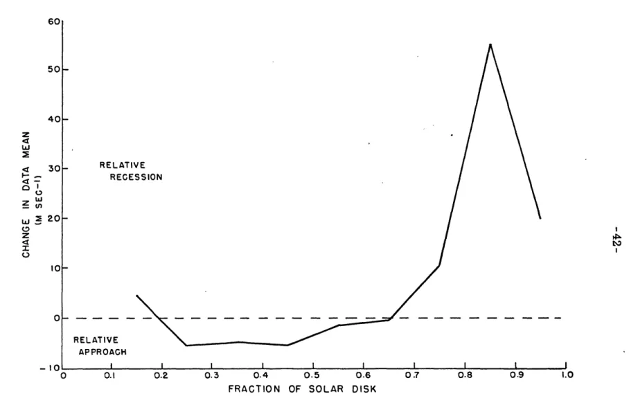
Center to limb variation in the mean Doppler velocity data determined for each annulus from all available measurements.

Final data averaging configuration and location of the integration paths.

Sample flow pattern which results when "Y is assumed to be zero along the equator.

Comparison of the flow patterns obtained when selecting Y* from the innermost and outermost integration paths.

Comparison of the flow patterns obtained from streamfunction calculations starting on the equator in the eastern and western hemispheres.

Comparison of the flow patterns obtained from equivalent sectors divided into 4, 8, and 12 equal parts prior to averaging.

Final version of the flow patterns for the period 30 June - 14 July 1972.

Scatter plot comparing meridional velocity components obtained from the flow patterns with those inferred from the daily proper motion of sunspots.

The location of calcium plages and sunspots in the large-scale flow patterns.

19 41 42 46 50 57 59 62 65 87

LIST OF FIGURES (continued)

Figure 12.

Figure 13.

Figure 14.

Flow in the vicinity of an active region inferred from various solar measurements

The day to day variation in the mean values of the zonal velocity between ± 300 latitude and the

covariance between the zonal and meridional velocity components at 1300 latitude.

The day to day variation in the mean values of the zonal velocity between 1300 latitude and the

covariance between the zonal and meridional velocity components which lie in the latitude belt bounded by 100 and 300 in both hemispheres.

103

108

LIST OF TABLES

Table 1. Sample distribution of data points within annular

rings representing multiples of equal surface area. 37 Table 2. Sample distribution of data points within annular

rings representing multiples of equal disk area. 38 Table 3. Sample distribution of data points within annular

rings of equal width. 40

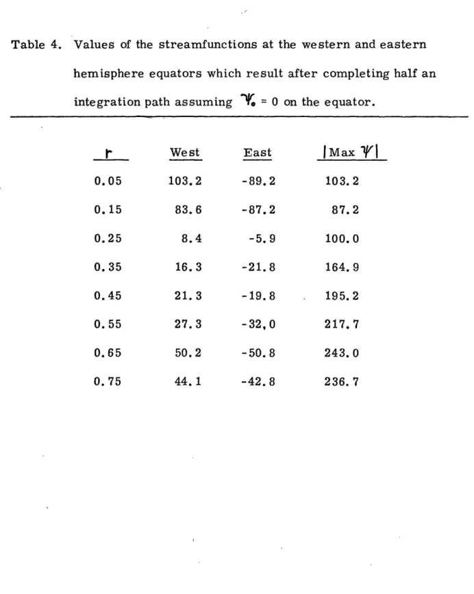
Table 4. Values of the streamfunctions at the western and eastern hemisphere equators which result after completing half an integration path assuming

4'

= 0

on the equator. 44

Table 5. Change in the value of ' on successive integra-tion paths corresponding to the mean net circulaintegra-tion

1. Introduction

1. 1. The Solar Differential Rotation and Efforts to Explain It Prior to 1964 the only documented variation in the solar rotation rate was a function of latitude. This "differential" rotation was first observed by Carrington in 1863 and refined over the following nine de-cades culminating in the form obtained by Newton and Nunn (1951).

Their result was based on the interval between successive central merid-ian passages for long-lived, recurrent sunspots from six solar cycles and essentially confirmed Carrington's initial finding -- the solar rota-tion rate was solely a funcrota-tion of latitude.

Newton and Nunn were aware that their particular subset of sun-spots produced a result which differed from those obtained from other subsets, but they judged the long-lived recurrent spots to be the most reliable tracers of the photospheric motions. Velocity profiles obtained using spectroscopic methods (Plaskett, 1952, 1954, 1959; Kinman, 1953; Hart, 1954, 1956; Adam, 1959) while agreeing with the sunspot rotation rates in the mean, contained the suggestion that the solar rotation rate was not as longitudinally invariant as the accepted profile would suggest.

Theories attempting to explain the differential rotation which had evolved concurrently with the observations were generally based on this

axisymmetric picture and reproduced the observed equatorial accelera-tion. Such theories appeared to be adequate when considered in a mean qualitative sense, but were deficient in most quantitative aspects.

A new approach to the subject was suggested by Ward (1964, 1965a) who viewed the mean solar rotation as the largest of a continuous spec-trum of size and velocity scales. Scales of motion smaller than this, he asserted, should not be viewed as noise to be averaged out; rather they are fundamental to the energetics of the solar circulation. Ward postu-lated the existence of a hierarchy of eddies in the solar atmosphere ranging in size from a fraction of the solar radius to a few hundred kilo-meters and sufficiently organized in space and time to maintain the mean circulation.

Citing results from laboratory experiments and analogous situa-tions in the earth's atmosphere, Ward argued for the existence of a

Rossby circulation regime in the solar atmosphere. As corroborating evidence for this contention, he analyzed the daily proper motions of

sunspots for one solar cycle and obtained positive correlations between deviations from the space and time averaged meridional and zonal com-ponents of these motions. Such a correlation, Ward concluded, implies a horizontal transport of angular momentum up the angular velocity gradient (towards the equator), a phenomenon known to exist in the

earth's atmosphere (e.g., Starr, 1968). The circulation pattern associ-ated with such a transport requires a solar rotation rate which varies in space or time or both.

Starr and Gilman (1965a, b) utilized Ward's findings in addition to maps the photospheric magnetic field to infer the direction and

magnitude of the angular momentum transfer as well as to speculate on the shape and orientation of perturbations in the zonal flow field. Such a process could be similar to those which maintain the circulation of the earth's atmosphere and generally cause marked deviations from mean conditions in both space and time. They further speculated that

hori-zontal Maxwell stresses converting the energy of the mean flow into the energy in the large scale magnetic patterns were acting to retard the equatorial acceleration. The net transport represents a balance between

competing processes.

Since then, the evidence to support the contention that the solar rotation varys in space and time has been accumulating from other sources, e.g., magnetic field data (Wilcox and Howard, 1968; Wilcox and Colburn, 1969; Stenflo, 1972) and velocities obtained from Doppler shifts (Plaskett, 1966; Howard and Harvey, 1970; Howard, 1971,

1972, 1973).

Despite the recent evidence to the contrary, there are those who continue to maintain that the deviations from the mean solar rotation are not basic to the underlying energetics. These variations continue to be

ignored even though their magnitude approaches that of the differential rotation itself. Such theories continue to rely on an axisymmetric circu-lation regime but unlike similar theories in the past, the meridional cir-culations are not constrained to conserve angular momentum. These models are based on the asumption that motions experience certain

anisotropies in basic properties, e.g., eddy viscosity (Kippenhahn, 1963; Cocke, 1967), conductivity (Durney and Roxburgh, 1971). These anisotropies as modeled produce meridional circulations transporting angular momentum towards the equator. However, all are characterized by an eddy viscosity and require negative viscosity coefficients at some point to produce consistent energetics (Gilman, 1974). Some parameter-izations introduce into the mathematical model the necessary effects of eddies while not fully exploring the physical implications. The resul-tant pitfalls of this approach have been discussed recently by Starr (1973a).

Other recent attempts to explain the maintenance of the solar differ-ential rotation are based on investigations of the full eddy regime. These theories tend to be more quantitatively well developed than the

axisym-metric type. Two mechanisms are considered; the distorting effect of rotation on "giant" convective cells (Kato, 1969; Busse, 1970;

Davies-Jones and Gilman, 1970; Yoshimura, 1971; Gilman, 1972; Heard and Veronis, 1974) while the other considers the presence of baroclinic instabilities (Gilman, 1969; Kato and Nakagawa, 1969, 1970; Suess, 1971). Both types successfully reproduce the observed equatorial acceleration and transport angular momentum towards the equator. For the assumed geometry and physical parameters, both mechanisms pro-duce large-scale features with dimensions in general agreement with those inferred both from Doppler velocity measurements (Howard, 1971) and from photospheric magnetic fields (Starr and Gilman, 1965b). The

particular shape (longitudinal rolls) of this large-scale feature suggested by the Doppler velocity measurements presently favors the giant cell models (Piddington, 1971; Gilman, 1972) although Suess (1971) has inter-preted these same patterns in terms of Rossby-type waves. Observed whole sun magnetic variations, e.g., field reversals, have been modeled with some success itilizing a dynamo based on Rossby wave dynamics

(Gilman, 1969; Gordon, 1972).

Encouraging as the results of such models are, they are not without their shortcomings. Generally the assumptions made in order to solve the complex systems of equations place restrictions on the character of the solutions to the extent that their applicability to the sun is uncertain at best. More explicitly, the models either assume or produce certain features which, if present, ought to be evident from the available

obser-vations. One example of such a feature which pertains to both theories is the presence of an equator to pole temperature gradient. The Rossby wave theories usually assume the existence of such a gradient to provide the energy for the resulting instability (Gilman, 1969) while the giant cell theories produce such a temperature gradient (Davies-Jones and Gilman,

1970; Gilman, 1972). The gradient in either case is approximately 50K and most recent measurements fail to confirm its existence (Altrock and Canfield, 1972; Canfield, 1973). Durney (1972, 1974) maintains that the pole-equator difference in flux produced by the convective models would

surface due to a reduction by a counter cell higher up rising at the poles and sinking at the equator. At least one Rossby wave model exists (Kato and Nakagawa, 1969) which does not assume the existence of a tempera-ture gradient. Instead, the waves are considered to be perturbations relative to a system rotating at a constant rate.

The mean meridional circulation characteristic of the giant cell models presents another discrepancy; most models contain a mean equa-torward flow (Gilman's is poleward). The observational measurements of mean meridional velocities either from sunspot data (Ward, 1964, 1973) or Doppler velocity data (Howard, 1971) have not yielded such circula-tions although the Doppler measurements are not sufficiently precise to

-1 detect motions of the magnitude required (N3m - sec ).

Clearly, all the theories proposed to explain the energetics of the solar general circulation cannot be entirely correct. Some combination is likely, for example, with convection in the interior producing a baroclin-ically unstable layer at the surface (Starr, 1973b). Such a system would combine a pole to equator temperature gradient (in this case at some level below the visible surface) produced by the giant convection cell theories with the non-axisymmetric flow characteristic of baroclinic instabilities. This particular combination would not violate any observations as they are presently accepted.

1. 2. Contribution and Scope of the Present Work

explain the solar general circulation contains one or more features which has not been observed in the solar atmosphere. Unfortunately, the

mea-surements of solar features are not themselves without difficulties. Efforts to observe a pole to equator temperature difference are made

more difficult by the lack of assurance that the optical solar limb is also a surface of constant heliopotential. Alternatively, if a dynamically im-portant temperature difference exists in the solar interior, direct obser-vation will be impossible.

One of the major problems still existing is the lack of sufficient observations of the motions (particularly meridional) which exist in the solar atmosphere. Even the mean rotation rate, first observed over a century ago, is no longer a sufficient description of motions in the photo-sphere much less the entire sun. There is probably no one rotation rate which canbe applied to the sun as a whole since the mean conditions appear

to vary with depth in the atmosphere (Wilcox and Howard, 1970). Even less well known are the short-termvariations in latitude, longitude and time (Livingston, 1969; Howard and Harvey, 1970; Howard, 1971, 1972, 1973) which are relatively recent determinations.

Instantaneous horizontal velocities can be obtained from motions of visible tracers and (at least theoretically) from Doppler shifts of spectral lines due to mass motions along the line-of-sight. Each technique has its own shortcomings which contribute to the uncertainty of the results. The difficulties encountered when attempting to determine instantaneous velocity

fields from sunspots are more acute than when determining mean motions. These include the lack of a sufficient number of tracers at a given time, non-random distribution of sunspots in the flow field and the probable

re-tardation of sunspot motions due to the presence of a magnetic field and the interchange of matter between sunspot and flow field. Further com-plexity is introduced since the degree to which sunspots fail to be ideal tracers varies with solar cycle and the stage of sunspot development (for a more complete discussion see Ward, 1965b; 1966a, b; 1967; 1973). Ve-locities obtained spectroscopically are free from these limitations. How-ever, the technique is accompanied by its own particular difficulties

(Howard et al., 1968) which will be examined in more detail in following sections.

The lack of sufficiently well determined motions in the solar atmo-sphere has contributed to the variety of solar circulation theories which have emerged. The basic difference between the non-axisymmetric the-ories and those based on primarily axisymmetric flows concerns the rela-tionship between space and time deviations from the mean solar rotation rate and the underlying energetics. Proponents of the axisymmetric the-ories minimize the importance of deviations, providing mechanisms to maintain the equatorial accelerations from mean circulation regimes. On the other hand, proponents of non-axisymmetric theories accept the exis-tence of significant space and time variations in the solar rotation rate and assign to these deviations major roles in maintaining the mean circulation.

The energy associated with these variations in the rotation rate are orders of magnitude greater than that associated with other available forms, e. g., magnetic energy. If such variations are fundamental to the energetics of the solar circulation, there will be detectable relationships which exist between the large-scale flow pattern and other observable features.

The scope of the work described herein is to obtain for the first time instantaneous large-scale flow patterns in the solar photosphere as they are inferred from daily Doppler line-of-sight velocity measureme nts. A description of the analysis technique, the preliminary data processing and the experiments performed to bridge the gap from theory to practice are contained in the following two chapters.

Daily flow patterns for a two week period in 1972 are presented and discussed in the fourth chapter which also contains more quantitative judgments of their overall validity based on comparisons with observa-tions of other solar phenomena. Estimates of the momentum transports

associated with the flow characterization are related to the observed variations in the daily determined mean rotation rate. The implications of these results as they pertain to the energetics of the solar general cir-culation along with suggestions for future research are the topics of the final chapters.

2. Obtaining Photospheric Streamlines from Solar Observations 2. 1. Technique

Velocity fields in the solar atmosphere may be obtained by measur-ing Doppler shifts in selected Fraunhofer lines. These Doppler shifts are due to motions within the line forming layer along the line-of-sight and as such render invisible components of the motions which are normal to this direction. When viewed from the earth, purely horizontal and vertical solar motions are undetectable at the central meridian and limb respec-tively. Alternatively, the line-of-sight velocity contains an increasing

portion of a purely horizontal velocity field as the observation approaches the solar limb.

A technique to infer the continuous horizontal flow field from this type of photospheric velocity measurement has been suggested by Gilman

(1971). Basically, the procedure assumes the flow along the solar sur-face to be horizontal, two-dimensional and nondivergent. Momentarily setting aside questions concerning the applicability of such assumptions, the horizontal divergence can be expressed, following Gilman, as:

S(V.Vx

cos e)

where V is the velocity and A and

0

denote the solar central merid-ian distance and latitude respectively (see Figure 1). A streamfunction Y

WEST LIMB

VA

-

;

> = cose I (2)

The line-of-sight velocity, V , is related to V. and Ve by:

VA

= - s1

r

V-

si

cos

Ce

V

(3)

or

Va

=

_sin

_'

_{- tant}

_cosA

_A

(4) which upon integration becomes

V

=

+

,

S

(5)

The paths of integration are such that

COS A Cos e = constant (6)

which for the sun are circles centered on the sub-earth point.

In equation (5), the constant of integration V is unspecified and differs for each integration path S . In order to produce a continuous solution for the entire solar disk, these arbitrary constants must be re-lated to one common but still unspecified constant. Gilman suggested as a first approximation that

Y

be set equal to zero along the equator. Such a stipulation prohibits flow across the equator.

A test of the technique was performed on terrestrial wind data by Fischer (1971). Utilizing six month summertime mean wind components for the half of the northern hemisphere centered on the Atlantic Ocean, he computed the line-of-sight velocity component apparent to an extrater-restrial observer and used Gilman's technique to infer the streamline pattern.

Direct application of the procedure resulted in small non-zero values for V at the termination of each integration path (semi-circular in this case) and were attributed to the presence of a small divergent component, cross-equator flow or both. It was not possible to estimate the contribution due to each but their effect was removed by subtracting the mean wind from the data. Overall agreement between the actual mean wind field and the flow patterns produced by the technique was favorable, encouraging its extension to an analysis of solar velocity fields.

2. 2. Solar Data Utilized

Forming the basis for this work are instantaneous line-of-sight velocities inferred by measuring Doppler shifts in the neutral iron line

(FeI) at

A

5250. 216 formed in the solar photosphe re. Daily whole disk measurements are made at Mt. Wilson Observatory and have been

de-scribed in a series of papers (Howard et al, 1968; Howard and Harvey, 1970; Howard, 1971, 1972). These measurements are configured in a rectangular grid 135 points wide, 108 points high of which approximately

point is approximately 0. 17 seconds of arc while the distance between grid points is roughly one and a half degrees of solar latitude.

Doppler shifts when observing a solar spectralline from the earth occur whenever relative motion exists between the observing instrument and the volume of gas in Which the line originates. Not all motions which contribute to the observed shift originate in local velocity fields on the sun. The rotation of both the earth and sun as well as the orbital motion of the earth contribute to the observed Doppler shift. In addition, the reddening of a solar spectral line as it is observed progressively limb-ward contributes an apparent shift as do a variety of instrumental effects. A complete discussion of the instrumental contributions appears in Howard and Harvey (1970) and will not be considered here. However, it is instruc-tive for a better understanding of the streamline patters being sought to review briefly how these and other contributions to the observed Doppler shift are removed before the resulting motions can be attributed to the solar atmosphere.

The line-of-sight velocity VL obtained from the observed Doppler shift in the FeI line is assumed to be the combined effect of relative

motions (real or apparent) between the line-forming layer and the observ-ing instrument and are accounted for by Howard and Harvey (1970) as the sum of individual contributions in the following manner:

VA

"(ai

6I1t9

+I C Srinle) R Cos 9cos 0B. SinA

4. o.32511 sp

4cosS-

24.189 sin(L.-L +

d + e(1- CosS

+

Vs,

A description of the origin of each term follows.

0 Contribution from the mean solar rotation

The mean solar rotation is one of the quantities under current inves-tigation at Mt. Wilson Observatory. It is determined on a daily basis along with several other parameters by evaluating the constants

a

, b and C from each day's measurement. The long term value is the mean of the individual values for the period of determination. The functional form for the latitudinal dependence is guided by the differential rotation

profiles obtained from sunspot motions. Term

0

in Equation (7) repre-sents the component of the mean solar rotation in the line-of-sight. Other quantities previously undefined are R , the radius of the sun and ,

the heliographic latitude of the sub-earth point.

©

Contribution from the earth's rotation

If the observation is taken prior to local noon, the rotation of the earth produces a slight component of motion towards the sun. Observa-tions made after local noon contain the reverse effect. The appropriate component in the line-of-sight is proportional to the well known astronom-ical constants H , the hour angle at observation time, and

S

the declination of the line-of-sight with respect the ecliptic plane. Knowing

the date and time of the observation as well as the geographic location of the observatory are all the quantities necessary to calculate this compo-nent of relative motion. Sufficiently precise determinations of this com-ponent are obtained by basing all calculations on a mean sideral day.

Q

Contribution due to the orbital motion of the earth Both ecliptic plane components of the orbital motion contribute a relative sun-earth motion. The earth-sun distance varies throughout the year resulting in a small day to day relative motion. Over the 90 minute interval required to take an observation this motion is below the limits of detectability and is ignored. The tangential component represents the difference between synodic and sideral rotation rate of the sun and is represented by term G with L. and L the celestial longitude of the center of the solar disk and line-of-sight, respectively. The earth's

orbit around the sun is assumed to be a perfect ellipse with the sun at one focus. Other minor effects which have been neglected are the sea-sonal variations in the linear sideral velocity of the earth in its orbit and the celestial latitude of the line-of-sight, B . This latter effect would be represented by an additional factor, cos B , in term ( . However,

since

B

is always near zero degrees, cos B is assumed always to equal one. As was true for the preceding term, the relative motion between the earth and sun due to the earth's orbital motion can be

calcu-lated from known astronomical quantities and is not determined as a result of the observation.

@ Reference level

In its present version, the Mt. Wilson instrument measures the wavelength shift in the FeI line only. If this shift was entirely due to lo-cal motions on the sun (after accounting for the other known effects), the absolute velocity between the plasma and the observer would be directly proportional to the observed line shift. Unfortunately, the shift as mea-sured contains unknown contributions from the terrestrial atmosphere and instrumentation. These effects must be removed before the velocities in the solar atmosphere are estimated. This removal is accomplished by determining a reference level, term M , which represents the aforemen-tioned effects on an observation of a stationary sun. The individual

mea-surements are then reckoned with respect to this reference level. To be effective, this reference level should remain constant over the span of time required to make the observation. The overall contribu-tion to the noise attributable to mechanical components, e. g., backlash,

ought to be near zero due to the boustrophedonic nature of the scan. More troublesome may be a net drift in this reference due to changes in atmos-pheric pressure during the course of an observation. A change of

0. 1 mm Hg in pressure produces a drift in the reference of nearly -1

60 m - sec . This effect would tend to produce a random noise com-ponent in studies dependent on averaging many measurements over a long period to determine, say, the long term mean rotation rate. Since these observations were made with such long term determinations in mind, no

pressure correction was made and its effect on daily measurements is unknown.

A future improvement which will allow a direct determination of the portion of the line shift which is not solar in origin is the simultaneous monitoring of a nearby spectral line which is formed in the earth's

atmo-sphere. Any shifts 'in the wavelength of the telluric line is then attributed to atmospheric and instrumental effects. A corresponding correction is

applied to the solar line at each point which removes all non-solar contri-butions from the measurements and allows absolute velocities to be

determined.

O

Red shift contribution

It is well known that the wavelength of a solar spectral line shifts towards the red as the observations are taken at points progressively nearer the limb. This center to limb variation (which is actually a blue shift towards the center) was originally thought to be due to preferential sampling of warm convecting elements. Such an explanation requires a center to limb variation proportional to ( I - CoS T ), where ? is the central angle. Observations, however, did not support this contention. Instead, Adam (1959) found the best fit was obtained assuming a parabolic proportional to ( I-coS 9 ) . This functional form is used in the

Mt. Wilson data reduction technique to predict the degree of red shift to be expected in the data. The unspecified constant,

e

,like those pre-ceding is determined by the daily data.

The entire limb reddening variation is undergoing a careful

re-examination by Hart (1974) utilizing the vast amount of data resulting from the Mt. Wilson observing program. A new theory is being tested which contends that the line shift observed is due to the combined effect

of Van der Waals and Lennard-Jones potentials. Such an effect is propor-tional to the density of the environment in which the line originates and in the case of the sun would produce a shift to the blue at the center of the disk since the radiation originates from deeper and therefore denser levels. The wavelength variaticrs from center to limb predicted for se-lected spectral lines have produced better agreement with the observations

than the ( I - cos P ) form presently used.

©

Motions in the solar photosphere

The final term, VSM , represents the velocity component due to deviations from the daily profile of the mean rotation. If the daily zonal velocity field, L. , is decomposed into its mean value 3 and

deviations (/) , i. e.,

U. =

u3

+

L/

(8)

term 0 represents the LL component,

EIU

already being accounted for by term 0 in Equation (7). Also included in VSM are the line-of-sight

components of any meridional and vertical (radial) motions which may be present.

The daily array of observations is analyzed by a least squares tech-nique with VsM treated as a residual. Once a solution is obtained and

the daily values for constants

a

through

e

determined, Vs, is cal-culated for each grid point. The daily data obtained from Mt. Wilson Observatory consist of values for VaS at each grid point as well as for the constants

a

,

b

, C , and e . Solutions are obtained determin-ing the rotation rate constants for the northern and southern hemispheres independently as well as for the disk as a whole.

A data reduction technique of this type is well suited to a study of the mean rotation rate but has certain disadvantages when subjected to a day by day analysis such as that at tempted by the present study. Since

VSa is treated as a residual, it also contains any noise components, random and non-random, which remain if the foregoing considerations have been insufficiently precise. Any unconsidered effects traceable to variations in atmospheric transparency and instrumental sources would probably alter the reference level in a uniform manner and produce little effect in the data for a given day. On the other hand non-random contri-butions, for example, the drift in the reference point due to changes in atmospheric pressure, would produce a slightly inhomogeneous data set during the 90 minutes it takes to obtain a complete disk scan. The mean of such a variation would become part of the reference level but a small non-random component could remain behind.

2. 3. Applicability of the Technique to the Solar Case

Before proceeding further with a description of the steps involved in producing daily flow patterns fr m solar line-of-sight velocity

measurements, a consideration as to the applicability of the technique to the solar case seems appropriate.

At first glance the assumptions upon which the technique is based, namely horizontally two-dimensional and nondivergent flow appear

vastly inadequate to faithfully represent motions in the solar photosphere. It is well accepted that the solar photosphere is primarily a convective layer from which radiation is being lost to space so rapidly that energy must be transported by convective rather than radiative processes. The theoretical criterion for stability against convection (Aller, 1963) is

d(lin

K

dIn T)]

(9)

S(In

P)

_PHoTosPOERE

d(In

P)

_{-AD 16TrIC}

From models of the photosphere (c.f., Allen, 1963) this criterion is generally met only for the uppermost layer of the photosphere between optical depths It 0. 004 (defining the base of the chromosphere) and 0. 8 (^ 280 km below). It is in this thin, stable layer where the Fraunhofer lines are formed.

Undoubtedly, the actual conditions are not as orderly as a model of the photosphere would suggest. Convection from below most likely pene-trates the underside of the stable layer and induces vertical motions

within it much like tropospheric convection penetrates into the stratosphere. While the density is not discontinuous at the top of the photosphere, it falls off rapidly enough throughout the lower layers of the chromosphere

to enable the surface of the sun to be treated as a free surface with no flow across it. When dealing with sub-sonic motions in.the solar photo-sphere, the flow may be treated as incompressible (Nakagawa and

Priest, 1973).

Expanding the vertical component of motion in terms of a mean taken around latitude circles (

£

] ) and deviations therefrom ( ' ), the continuity equation becomes

+

-

+

(10)

since 1%0

If motions on the scale of the convection are being considered, Equation (10) would have to be applied as written. However, the intent

of this analysis is to depict the large scales of horizontal motion assum-ing that there is no ordered vertical motions with so large a scale. The additional assumption is made that if the scale of the substantive convec-tion can be identified, the data representing an area occupied by several cells can then be averaged ( ) such that the resulting value contains very little contribution from the smaller scale convection, i.e., r ^ 0

Thus, if the radiation yielding the measurements originates fairly high in the photosphere near

t'-

0. 004 the assumptions that the flow is horizontally two-dimensional and nondivergent are generally good ones.

of the convection zone ( , 0. 8), the forcing by the strong underlying vertical motions may weaken the validity of those assumptions if the measurements are capable of resolving the convection.

A mean optical depth to can be defined such that one-half the radiation emerging from the surface originates above and one-half below this level. For a grey atmosphere, e- = 1/2 or t-, 0.69. Therefore, most of the radiation observed by the instrument originates slightly above the top of the convective zone and probably includes mo-tions influenced by the underlying convection. The success of the tech-nique in representing the large-scale velocity fields in the solar photo-sphere will depend inlarge measure on successfully removing the effects of this smaller-scale convection from the mean line-of-sight velocity data ultimately used to calculate the streamfunctions.

3. Producing Solar Flow Patterns

3. 1. Introducing a Solid Body Reference

The intent of this analysis is to construct large-scale flow patterns for the solar photosphere analogous to those depicted on constant pressure

charts representing flow in the terrestrial atmosphere. This similarity is desirable to facilitate the interpretation of the results, especially with an eye towards identifying any structure which may exist in the space and time variations from the mean solar rotation rate which these Doppler data seem to contain. In order to achieve such a product, it is necessary to refer the velocity fields in the solar atmosphere to an underlying solid body rotation rate.

The measurements as obtained from Mt. Wilson Observatory rep-resent the line-of-sight components of velocities in the solar photosphere except for that component arising from the daily mean rotation rate.

However, this mean itself changes from day to day (as the daily variation in

a

, b , and C indicate) and in doing so contributes to any varia-bility present. In order to achieve the stated objective a common

refer-ence must be selected.

At first glance, the rotation rate of the Greenwich coordinate sys-tem appears to be the obvious choice. However, this coordinate system reflects a mean rotation rate characteristic of recurrent sunspots which differs somewhat from that obtained by spectrographic methods. Rather than use a reference characteristic of another level, it was decided to

utilize the long-term mean rotation rate determined from the

spectrosco-pic data themselves. This mean rotation rate is (Howard and Harvey, 1970)

o,]= 2.78(o')-5-.51(I'7)

sie-

4.43('')sirfe seC' (11)

An overbar ( ) will be used to denote a time average. As an under-+o lying reference, the angular frequency of rotation corresponding to -20 was selected

[ool.]

=

.73

(to-')

see

(12)

The VS, , data were then adjusted point by point to re-introduce the line-of-sight component

AV

due to the difference in the daily and long term mean rotation rates. This adjustment was straightforward

A

V.

=

R

(CW

-

)

CoS

G

sI

~Ios

h

Bo

1-

sec

-i

(13)

Adhering to the Mt. Wilson sign convention, AVt is negative for approach and positive for recession. Defining solar velocities in this manner produces in the mean westerlies equatorward and easterlies

+o 0

poleward of -20 heliographic latitude. Directions here are reckoned in a terrestrial sense, i.e., zonal velocity fields in the same sense as the rotation are referred to as "westerlies". As will be discussed in more detail in sections to follow, the solar rotation rate for the period analyzed is greater than average resulting in a substantial poleward displacement of the boundary separating easterlies and westerlies.

3. 2. Minimizing the Effects of Small-Scale Convective Motions In section 2. 3 it was concluded that if a suitable area could be de-fined which would include more than one of the underlying convection cells,

the line-of-sight velocity data within this area could be averaged and the mean value contain little, if any, contribution from the vertical motions organized on the smaller scale. Prior to exploring the scale size of the convection present in the solar atmosphere, a determination of how best to uniformly represent various portions of the solar surface must be made.

Ideally, the solar surface should be uniformly sampled to avoid over-representing one portion of the hemisphere while neglecting others. Clearly this ideal goal is unattainable since the geometric realities of observing a sphere from a fixed point in space will always provide more direct access to that portion of the surface directly beneath the vantage point. For example, the half of the surface area lying limbwards of 600 central angle is represented by slightly less than 25%o of the area of the solar disk (the apparent area covered by any earth-based measurements).

Furthermore, the Doppler measurements suffer from an additional asymmetry. A given line-of-sight velocity contains a more direct mea-surement of actual horizontal motions when obtained near the limb than it does near the center of the disk. Therefore, the chance for contamina-tion by vertical mocontamina-tions is greater at the center than towards the limb. When representative line-of-sight values for the large-scale motion are being produced, more data points should be used to compute the mean near the center per unit surface area than near the limb to obtain values with similar residual effects. So the initial step in the averaging

roughly the same surface areas.

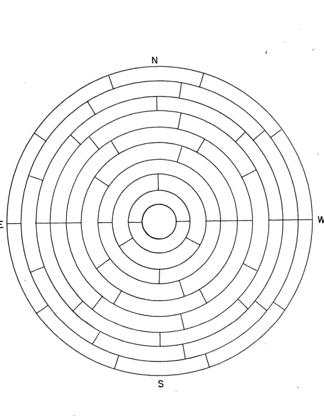
A practical consideration to the ultimate averaging technique was the circular geometry required to calculate the streamfunctions. It was necessary to provide mean values for the line-of-sight velocities on

circu-lar paths centered on the sub-earth point. Such a final configuration is directly achieved by dividing the disk into annular rings, then the rings azimuthally in some regular fashion and assigning the mean value of all data within each sector to the sector center of gravity. Alternatively, primary averaging could be accomplished maintaining a rectangular grid, then values obtained along circular paths by interpolation. Both approaches were tested and yielded similar results for identical integration paths. The purely circular method was preferred since it weighted each data point equally in producing the mean for the sector it represented while for the rectangular technique it was not clear how this could be accomplished while maintaining a truly independent procedure. Additionally, the circu-lar method is easily related to the fraction of the surface area falling within each sector, a distinct advantage in the analysis which follows.

Once having decided (albeit somewhat arbitrarily) on the geometri-cal form the averaging procedure will assume, the question concerning how best to represent the entire solar surface can be pursued. It has

al-ready been stated that while most desirable, strictly uniform sampling of the solar atmosphere for the entire solar hemisphere is unattainable. However, this does not prevent one from dividing the solar surface into

equal portions and utilizing the measurements which happen to fall within the projection of each to provide a mean value for each equal

portion. This approach would assure that a large number of data points were averaged over segments near the sub-earth point while fewer would determine the mean near the limb. This approach need not

pro-vide a realistic representation of motions towards the limb since the distribution of data points results in over-sampling the portions near the center of the disk while those portions near the limb are sparsely sampled or occasionally sampled not at all.

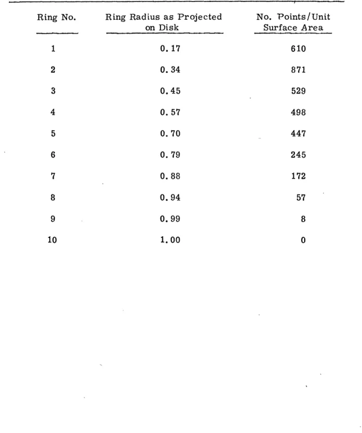
To be more specific, Table 1 contains, for the data distribution used in this study, the number of measurements per unit surface area as a function of central distance. The unit surface area was defined by dividing the solar hemisphere into ten annular rings concentric about the

sub-earth point (numbered one to ten from the smallest) such that the area of each annulus was equal to its number times the area of the in-terior circle (the unit surface area). The projection of these segments

onto the solar disk results in concentric circles with radii as indicated. The total number of data points within each annulus also appears. An examination of Table 1 makes obvious the fact that this approach over-samples portions near the center of the disk while near the limb the sampling rate declines drastically.

An attempt to temper the goal of equal area representation with the production of homogeneous means utilized an approach similar to the

Table 1. Sample distribution of data points within annular rings repre-senting multiples of equal surface area.

Ring Radius as Projected on Disk No. Points/Unit Surface Area 0.17 0.34 0.45 0.57 0.70 0.79 0.88 0. 94 0. 99 1. 00 610 871 529 498 447 245 172 Ring No.

Table 2. Sample Distribution of Data Points Within Annular Rings Representing Multiples of Equal Disk Area.

Radius on Disk 0. 134 0.234 0. 330 0. 424 0. 523 0. 618 0.717 0.809 0.904 1. 000 No. Points/Unit Disk Area 380 383 354 329 318 271 243 183 129 30

Area of Solar Sur-face Per Unit

Disk Area 0.0090 0.0095 0.0098 0.0100 0.0108 0.0111 0.0127 0.0135 0.0180 0. 0430 No. Points/0.01 Part Surface Area 422 403 361 329 294 244 191 135 71 7 Ring No. 1 2 3 4 5 6 7 8 9 10

previous one, namely dividing the solar disk into equal area segments. As Table 2 indicates the number of points per unit surface area declines more slowly as the limb is approached.

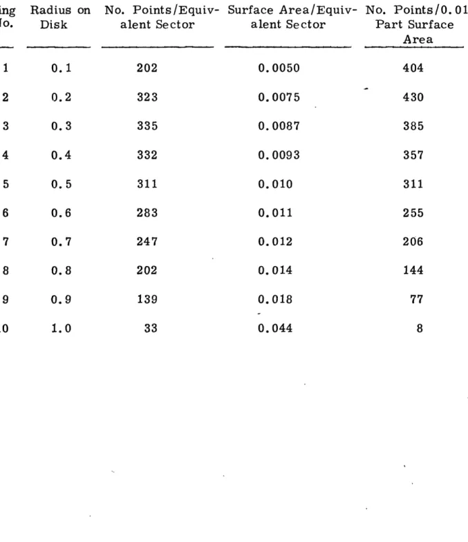
An additional attempt was made to lessen the decrease in the

number of data points per unit surface by setting the widths of the annular rings equal. Comparable data for this configuration appear in Table 3. The term equivalent sector will be used to denote the basic subdivision of each annular ring, i.e., 1, 2, . . . 10. Unit area is no longer

appropriate since the sectors are no longer of uniform size with respect to either the surface or disk. The fraction of the solar surface repre-sented by each (equivalent) sector varies by a slightly larger amount than in the arrangement represented by Table 2. However, the number of data points per unit surface area decreases at a slightly slower rate

in the vicinity of the middle rings.

The last method (see Figure 2) was adopted to preliminarily divide the data into sectors which when further subdivided into a given number

of equal parts would produce homogeneous mean values. The remaining question to be explored concerns the further subdivision of these equiva-lent sectors to adequately remove the convective motions while

attempt-ing to retain any structure which may exist in the flow.

While performing the foregoing analysis, it was discovered that a systematic center to limb variation existed within the line-of-sight data. Figure 3 depicts the difference between adjacent annuli of the mean value

Table 3. Sample Distribution of Data Points Within Annular Rings of Equal Width. Radius on Disk 0.1 0.2 0.3 0.4 0.5 0.6 0.7 0.8 0.9 1.0

No. Points/Equiv- Surface Area/Equiv- No. Points/0.01 alent Sector alent Sector Part Surface

Area 202 0.0050 404 323 0.0075 430 335 0.0087 385 332 0.0093 357 311 0.010 311 283 0.011 255 247 0.012 206 202 0.014 144 139 0.018 77 33 0.044 8 Ring No. 1 2 3 4 5 6 7 8 9 10

RELATIVE RECESSION 20- I0-RELATIVE APPROACH I I 0 0.1 0.2 0.3 0.4 0.5 I I ! I 0.6 0.7 0.8 0.9 1.0

FRACTION OF SOLAR DISK

Figure 3. Center to limb variation in the mean Doppler velocity data determined for each annulus from all available measurements.

401-

for the entire period of all points within the ten concentric circles. The pronounced increase in the mean line-of-sight velocity limbwards of 0. 8 central distance indicates that on the average the limb is receding with respect to the remainder of the disk,, clearly not a physical occurrenbe. There are similar trends near the center of the disk on certain days, most notably on 01, 09, and 14 July. However, since the center of the disk represents a continuous area, it is possible that there is some coherent motion in this area which results in a different value for this annulus average. This is almost certainly the case on 01 and 09 July when sunspots occur near the sub-earth point. (Howard observes pre-dominantly downward motion over active regions. ) However, in the case of the outer rings there is such a wide range of latitudes and longitudes represented that it is difficult to imagine a dynamic cause for a systema-tic recession of the outermost rings.

It is suggested that the limb reddening discussed previously con-tributes to this relative motion. The study by Hart may lead to a more precise accounting for this phenomenon which could reduce this systema-tic effect. Future improvements notwithstanding, it was decided to

utilize only that portion of the data out to a central distance of 0. 8. The data in these rings were normalized by subtracting the annulus average.

Having reached a decision on how best to represent the solar sur-face with the data at hand, it remains to determine how finely to divide

a priori to decide when all the effects of convection and other random noise have been removed, establishing the size of this optimum area depends as much on the appearance of the final product as on the physical dimensions of the most prevalent convective mode. The preliminary streamfunction calculations necessary to resolve this question were accompanied by their own peculiar set of problems which required solu-tion before any final judgments were possible.

3. 3. Mechanics of the Analysis

According to Equation (5), the difference in the streamfunctions between any two points along the path of integration is the integral of the line-of-sight velocity along the path length connecting the points in ques-tion. In order to apply this result to the present study the corresponding finite-difference approximation to Equation (5)

A

+

=

+

V

1,

)

AS

(14)

is used. The variables Y(i,) and Y. are the streamfunctions at successive points 44-1 and L separated a distance AS measured along

A

the arc over which a mean line-of-sight velocity Vt is observed.

There is no stipulation contained within (5) which restricts the man-ner in which AS is defined. The result should hold whether AS is large or small and ought not depend on a regular spacing providing the mean value for V is a faithful representation of the actual distribution of Vt

along ds . In the case under consideration, the foregoing analysis deal-ing with the most appropriate data averagdeal-ing technique provides mean values

Sat regular intervals around each circle, the final spacing dependent on the

number of subdivisions of the equivalent sector. Future results may suggest an advantage to be gained by nonuniform spacing between mean data points but none is apparent now and the present study will not consider such a case.

As mentioned, all streamfunctions are determined to an additive constant and the success of the procedure in producing a continuous field of values lies in being able to relate all streamfunctions to one common (but still unknown) constant. The absolute values are not necessary since the velocities are proportional to the streamfunction gradient.

As Gilman (1971) points out, one procedure which yields a continu-ous field of values (referred to in what follows as "closing" the technique) is the specification of the streamfunction along a curve which cuts all the integration paths. This immediately establishes a common reference for all paths, resolving the problem directly. Specifically, Gilman's sugges-tion that Io be set to zero along the equator (consistent with no flow across the equator) was adopted as a first try at closing the analysis tech-nique. This specification was used by Fischer when testing the technique on terrestrial data. While his ultimate result compared favorably with the flow pattern analyzed directly, some adjustment was required to insure

that V vanished identically when a semi-circular integration path (simi-lar to that between points

A

and B in Figure 4) was traversed. The source of the residual was not readily apparent; possible contributions included inadequate representation of data due to a coarse grid, the small

0,8 CENTRAL AVERAGING DISTANCE CONFIGURATION ... SLIMB CENTRAL MERIDIAN SUB-EARTH POINT EQUAT OR INTEGRATION : : :I: PATHS PORTION EXCLUDED FROM ANALYSIS

Figure 4. Final data averaging configuration and location of the integration paths.

cross-equator flow present in the sample and the divergence and vertical motions associated with convection. Since these processes have the potential for even greater impact on the outcome of the solar analysis, it was not entirely unextpected when the identical procedure proved to be inadequate in the trial run which follows.

A trial analysis was performed using the solar data with the equiva-lent sector divided arbitrarily into eight subdivisions. Since the stream-functions were to be calculated beginning on the equator, the subdivisions were chosen to assure that no resulting data would lie directly on the equator. The calculations were performed beginning at the equator in the eastern (left) hemisphere and proceeded in a clockwise direction. Both

choices, i. e., point of origin and direction, were arbitrary and as later comparison will show, other choices produced similar results.

A typical result of this analysis is contained in Table 4 which lists the values of the streamfunctions for the equator in the western and east-ern hemispheres respectively as well as the maximum value of "I cal-culated along each path. Recall that the calculation began in the eastern hemisphere with an assumed value of Vo = 0, then proceeded in a

clockwise direction. If the assumption that "T₀ = 0 along the equator were essentially correct, the values tabulated in Table 4 should be in the vicinity of zero. Even allowing for imperfections in both technique and data, this is clearly not the case. It is immediately apparent that there is a discontinuity in the flow pattern at the equator resulting from the

Table 4. Values of the streamfunctions at the western and eastern hemisphere equators which result after completing half an

integration path assuming

io

= 0 on the equator.

r West East IMax

K1

0.05 103.2 -89.2 103.2 0.15 83.6 -87.2 87.2 0.25 8.4 -5.9 100.0 0.35 16.3 -21.8 164.9 0.45 21.3 -19.8 195.2 0.55 27.3 -32, 0 217.7 0.65 50.2 -50.8 243.0 0.75 44.1 -42.8 236.7

assumed constancy of the streamfunction there (see Figure 5). The pattern in low latitudes for both hemispheres strongly suggests that flow

occurs across the equator on the sun. Questions regarding the reality of such flows, or more generally of the entire pattern, will be set aside until a more realistic appearing result is obtained.

The qualitative assessment of these initial results suggest the form of the next attempt, but more positive justification can be found in an examination of the calculations performed along each integration path. Note that the sums of the streamfunctions at the equator in the western and eastern hemispheres contained in Table 4 are relatively close to zero suggesting that mass continuity would be maintained along the horizontal surface when the net flow across closed circular paths is considered.

As was the case when testing the technique using terrestrial data, the value obtained at the completion of the integration is not precisely equal to that assumed at the start. Comparison of each residual (the sum of "T on the equator in both hemispheres) with the maximum value encoun-tered along each path gives an indication of their relative magnitude. With the sole exception of the innermost circle, the residuals represent less than 5 percent of the maximum value. The larger value associated with the innermost circle may be due to the presence of an active region in the vicinity of the sub-earth point on this particular day. A positive residual, if real, would indicate a net outflow of mass across the circle. This may very well be the case when an active region is enclosed since Howard (1971)

Figure 5. Sample flow pattern which results when " is assumed to be zero along the equator.

observes a downward motion at this level in the vicinity of active regions. If such motions represent material descending from above, a net flow across a closed path could occur.

To avoid the discontinuities which these residuals would introduce into the flow patterns, the line-of-sight velocities were adjusted to elimi-nate net flows across the closed paths. This adjustment consisted of subtracting V; from each mean line-of-sight velocity around the respective circle, where V the mean correction is defined as

V = Z (15)

-1

Generally, such corrections were quite minor, N 5 m - sec , although

S-1

for the innermost circle in the example given

V

1!s 30 m - sec .

With-out exception the highest corrections occurred on the innermost circles where the component of horizontal velocities in the line-of-sight is small. Thus, the chance for contamination by spurious effects and net vertical motions is greatest.

Relakation of the constraint prohibiting flow across the equator, while allowing calculation of continuous streamfunctions for each circle independently, leaves behind a more serious problem. There is no longer any a priori justification to specify the position of a streamline within the flow and, as a result, no direct relationship exists among the streamfunc-tions on each characteristic circle. It is mathematically correct to pro-ceed as before, i.e., assuming

'I'

= 0 on the (eastern) equator, but the resulting flow field would contain a barrier across which no flow may

occur. Clearly, there is no physical justification for this result, requir-ing that an alternative approach be sought to close the technique.

A solution to this problem can be found within the original definition of the streamfunction. In heliographic coordinates the components of ve-locity in the meridional (

0

) and zonal ( )directions are given in terms of the streamnfunction, " , by

V = -e j- Ve cose X (16)

If the heliographic coordinates are transformed into a new system, o and ? , where Q0 is the azimuth angle about the sub-earth point and ? is the central angle, the velocity components in the o(C and directions can be obtained (see Appendix A):

=Vc a (17)

Since dS=

dvdc

and Vj= t

V3

, the relationship defining is the differential form of Equation (5) from which the streamfunctions were originally defined. It follows then if V could be determined along

paths of constant o( , the variation of 'Y with ? would be specified and a continuous field of

Y

for the entire disk produced. Unfortunately,

Va( is everywhere perpendicular to the line-of-sight and is undetectable making a point by point determination of b T/B impossible.