HAL Id: hal-02394824
https://hal.archives-ouvertes.fr/hal-02394824
Submitted on 5 Dec 2019
HAL is a multi-disciplinary open access
archive for the deposit and dissemination of
sci-entific research documents, whether they are
pub-lished or not. The documents may come from
teaching and research institutions in France or
abroad, or from public or private research centers.
L’archive ouverte pluridisciplinaire HAL, est
destinée au dépôt et à la diffusion de documents
scientifiques de niveau recherche, publiés ou non,
émanant des établissements d’enseignement et de
recherche français ou étrangers, des laboratoires
publics ou privés.
E. Astafyeva, K Shults
To cite this version:
E. Astafyeva, K Shults. Ionospheric GNSS Imagery of Seismic Source: Possibilities, Difficulties, and
Challenges. Journal of Geophysical Research Space Physics, American Geophysical Union/Wiley,
2018, �10.1029/2018JA026107�. �hal-02394824�
Ionospheric GNSS Imagery of Seismic Source: Possibilities,
Dif
ficulties, and Challenges
E. Astafyeva1 and K. Shults1
1Institut de Physique du Globe de Paris, Paris Sorbonne-Cité, CNRS UMR 7154, Paris Cedex, France
Abstract
Up to now, the possibility to obtain images of seismic source from ionospheric Global Navigation Satellite Systems (GNSS) measurements (seismo-ionospheric imagery) has only beendemonstrated for giant earthquakes with moment magnitude Mw≥ 9.0. In this work, we discuss difficulties and restrictions of this method, and we apply for thefirst time the seismo-ionospheric imagery for smaller earthquakes. The latter is done on the example of the Mw7.4 Sanriku-oki earthquake of 9 March 2011. Analysis of 1-Hz data of total electron content (TEC) shows that thefirst coseismic ionospheric disturbances (CID) occur ~470–480 s after the earthquake as TEC enhancement on the east-northeast from the epicenter. The location of thesefirst CID arrivals corresponds to the location of the coseismic uplift that is known as the source of tsunamis. Our results confirm that despite several difficulties and limitations, high-rate
ionospheric GNSS data can be used for determining the seismic source parameters for both giant and smaller/moderate earthquakes. In addition to these seismo-ionospheric applications, we raise several fundamental questions on CID nature and evolution, namely, one of the most challenging queries—can moderate earthquake generate shock-acoustic waves?
Plain Language Summary
Ionosphere is a layer of charged particles of the Earth’s atmosphere located at altitudes ~60–800 km. However, despite being high above the Earth’s surface, the ionosphere is sensible to numerous near-ground geophysical events (earthquakes, tsunamis, volcano eruptions, etc). Acoustic and gravity waves emitted by these events propagate upward and generateatmospheric/ionospheric perturbations. Ionospheric disturbances generated by earthquakes are known as coseismic ionospheric disturbances (CID). Recently, it has been suggested that analysis of CID and theirfirst arrivals can provide information on the position and on the structure of seismic fault ruptured in
earthquake. This method is known as ionospheric imagery of seismic source. However, so far, this method has been only applied to giant earthquakes (Mw≥ 9.0). In this work, for the first time, we apply the ionospheric imagery for smaller earthquakes on the example of the M7.4 Sanriku-oki earthquake that occurred on 9 March 2011 in Japan. Our results show that this method is applicable to smaller earthquakes, and despite some difficulties, it can indicate the position of coseismic uplift ~8 min after the earthquake. The uplift generates CID but also tsunamis. Therefore, our method can be used as independent or
complementary one for near–real-time tsunami warning systems.
1. Introduction
It is now well demonstrated that earthquakes can generate perturbations in the ionosphere (e.g., Afraimovich et al., 2001, 2010; Astafyeva & Heki, 2009; Bagiya et al., 2018; Calais & Minster, 1995; Heki & Ping, 2005; Jakowski et al., 2006; Komjathy et al., 2016; Liu et al., 2011; Perevalova et al., 2014; Rolland et al., 2011; Zettergren & Snively, 2015). During an earthquake, a sudden impulsive forcing from the ground or oceanfloor generates atmospheric pressure waves that propagate upward into the ionosphere. These per-turbations are called co-seismic ionospheric disturbances (CID). Spatio-temporal and dynamic features of CID have been extensively investigated within the last decade by using signals of Global Navigation Satellite Systems (GNSS; e.g., Astafyeva et al., 2009, 2014; Bagiya et al., 2017; Ducic et al., 2003; Jin et al., 2010; Rolland et al., 2011, 2013).
Apart from systematic detection of earthquakes in the ionosphere, more recently, it has been suggested that CID can provide information on a seismic source (i.e., seismic fault region). For instance, Afraimovich et al. (2006) used an approximation of a spherical wave propagating from a point source at a constant speed and managed to show the position of a CID source in the vicinity of the epicenter of the 2003 Hokkaido
RESEARCH ARTICLE
10.1029/2018JA026107
Key Points:
• By applying the method of seismo-ionospheric imagery, we show the location of the seismic source for the Mw7.4 2011 Sanriku-oki earthquake
• We discuss possibilities, difficulties, and challenges of the method of ionospheric imagery of seismic source
• Simultaneous use of the ray-tracing technique and GNSS observations can be useful to resolve some difficulties of the ionospheric imagery Supporting Information: • Supporting Information S1 • Movie S1 Correspondence to: E. Astafyeva, [email protected] Citation:
Astafyeva, E., & Shults, K. (2019). Ionospheric GNSS imagery of seismic source: Possibilities, difficulties, and challenges. Journal of Geophysical
Research: Space Physics, 124. https:// doi.org/10.1029/2018JA026107 Received 18 SEP 2018 Accepted 7 DEC 2018
Accepted article online 14 DEC 2018
©2018. The Authors.
This is an open access article under the terms of the Creative Commons Attribution-NonCommercial-NoDerivs License, which permits use and distri-bution in any medium, provided the original work is properly cited, the use is non-commercial and no modifica-tions or adaptamodifica-tions are made.
earthquake in Japan. Similar method was later successfully applied by Shults et al. (2016) to localize of the April 2015 Calbuco volcano eruptions and to estimate the onset time of the eruptions from ionospheric GNSS measurements. Liu et al. (2010) suggested a method based on the ray-tracing and the beam-forming techniques and successfully localized the epicenter of the 1999 Chi-Chi earthquake in Taiwan from iono-spheric Global Positioning System (GPS) data. Lee et al. (2018) used for thefirst time ionosphere-based back-projection method to estimate the location of the seismic source of the 2016 Kaikoura earthquake in New Zealand.
Even closer relation between CID and a seismic source structure was shown for recent giant earthquakes with magnitudes Mw≥ 9.0. Heki et al. (2006) analyzed ionospheric total electron content (TEC) response to the great M9.1 2004 Sumatra earthquake and reproduced the rupture process. Astafyeva et al. (2011) used 1-Hz GPS-TEC data and, on the example of the Mw9.0 2011 Tohoku-oki earthquake, obtained for thefirst time the ionospheric images of seismic fault. Astafyeva, Rolland, et al. (2013) showed that ionospheric mea-surements can provide information on a seismic source location and even on the source dimensions within ~8 min after an earthquake in case if we detect direct acoustic waves above the epicentral area. In addition to that, Astafyeva, Rolland, et al. (2013) demonstrated that plotting standard snapshots of TEC over the epicen-tral area is useful to retrieve the information about the seismic source structure. Thus, for the case of the 2011 Tohoku-oki earthquake, two areas of enhanced TEC simultaneously occurred at ~150 km eastward from the epicenter ~520–530 s after the earthquake (Astafyeva, Rolland, et al., 2013). The location of these two TEC enhancements corresponded to the location of two segments of coseismic uplift as was shown by seismolo-gists (Bletery et al., 2014; Simons et al., 2011).
It is important to emphasize that ionospheric information about seismic source can be obtained shortly after an earthquake, within ~8–9 min. In such a case, the CID information could be used for tsunami alerts in the near real time, since CID are generated by a seismic uplift that also generates tsunamis. However, while we are talking more and more often about ionosphere-based tsunami warning systems (e.g., Kamogawa et al., 2016; Savastano et al., 2017), it is now of highest importance to understand possibilities and limitations of seismo-ionospheric methods. It is especially critical knowing that our knowledge on CID generation over the epicentral area is not yet quite sufficient. Also, most of studies were devoted to giant earthquakes such as the Mw9.1 2004 Sumatra or the Mw9.0 2011 Tohoku-oki events, whereas smaller magnitude earthquakes that occur much more often but nevertheless can lead to catastrophic damages and tsunamis, received less attention from the community.
The main focus of this work is to study the possibility of ionospheric GNSS imagery for smaller earthquakes and to examine difficulties and restrictions of the suggested method. The former is done on the example of the Mw7.4 2011 Sanriku-oki earthquake by using high-rate 1-Hz ionospheric TEC data from Japanese net-work of ground-based GPS receivers GEONET (GNSS Earth Observation Netnet-work System).
2. The Mw7.4 Sanriku-Oki Earthquake of 9 March 2011
On 9 March 2011, at 02:45:20 UT, a large thrust earthquake of a moment magnitude 7.4 shook the middle portion of the Japan trench. With hypocenter depth of 32 km, this shallow earthquake had an epicenter at point 38.435°N, 142.842°E (https://earthquake.usgs.gov/earthquakes/eventpage/usp000hvhj#). Shao et al. (2011) calculated the hypocenter position to be at the depth of 14 km in the point with coordinates (38.34°N, 143.12°E). Seismological models estimated the seismic slip reaching up to ~2 m at ~20–40 km on the northwest from the epicenter (e.g., Shao et al., 2011; http://earthquake.usgs.gov; Figure 1a). One of the most important seismological characteristics of an earthquake is the magnitude and the position of coseismic crustal vertical displacement that serves the source for generation of tsunamis and CID. Thomas et al. (2018) estimated the coseismic deformation pattern due to the Sanriku-oki earthquake as subsidence on the west-northwest from the epicenter and uplift on the east from the epicenter. The maximum uplift of ~0.3 m was located ~20 km from the epicenter (here shown by white cross in Figure 1a).
The Sanriku-oki earthquake caused a small tsunami runups up to ~0.6 m in Ofunato, Japan (https://www. ngdc.noaa.gov/). Note that the Sanriku-oki earthquake occurred 51 hr before the Mw9.1 Tohoku earthquake and is often referred to as the Tohoku foreshock.
3. Results and Discussions
3.1. Ionospheric Response to the Sanriku-Oki Earthquake of 9 March 2011
The dispersive property of the ionosphere makes it possible to estimate TEC from the linear combination of carrier phase and code dual-frequency GNSS measurements (e.g., Calais & Minster, 1995; Hofmann-Wellenhof et al., 2008). TEC is measured in TEC units (TECU), with 1 TECU equal to 1016electrons/m2. In this paper, the estimated slant TEC was converted to vertical TEC (Klobuchar, 1986). The elevation cutoff was set to 15°. To extract the CID signatures, we used the running meanfiltering method that works as band-passfilter in the range 0.5–6 min.
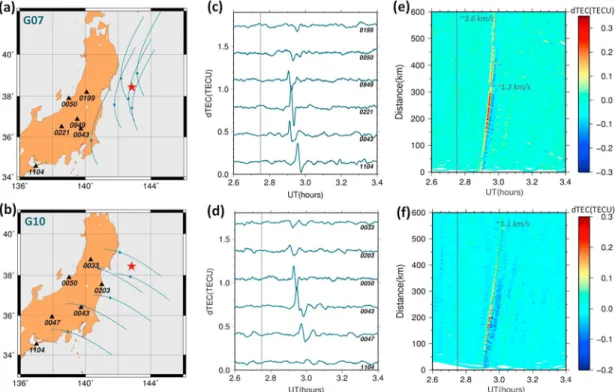
During the Sanriku-oki earthquake, several GPS satellites were visible by ground-based GPS receivers of the GEONET. However, here we focus on the near-epicentral area, and therefore, we only discuss measure-ments by GPS satellites G07 and G10.
Figures 2a and 2b show the geometry of GPS sounding for satellites G07 (a) and G10 (b) during the 9 March 2011 earthquake. The corresponding TEC measurements for GPS satellites G07 and G10 can be found in Figures 2c and 2d. One can see that the waveform of the observed TEC signal varies depending on the sounding position relative to the epicentral area. On the north, we mostly observe smaller amplitude signals and small TEC depletions. On the south, the TEC response shows a typical N-waveform with larger amplitude. The dif-ference in the CID waveform with respect to the seismic source is usually explained by the impacts of the mag-neticfield on CID propagation and by the geometry of GPS-sounding, and has been extensively discussed in previous works (e.g., Afraimovich et al., 2001; Bagiya et al., 2017; Heki & Ping, 2005; Rolland et al., 2013). The traveltime diagrams for observations from satellites G07 and G10 are shown in Figures 2e and 2f, respec-tively. We see good correlation with the earthquake’s epicenter that confirms that the observed ionospheric TEC perturbations were generated by the earthquake. From these diagrams we estimate the horizontal CID
Figure 1. (a) General information about the Sanriku-oki earthquake of 9 March 2011. The epicenter is shown by red star; the position of the maximum of the coseismic crustal uplift is depicted by white cross (data from Thomas et al., 2018). The magnitude of the coseismic slip is shown by colored dots around the epicentral area, and the corresponding color scale is shown below the panel (the data are from the U.S. Geological Survey, http://earthquake.usgs.gov). The focal mechanism of the Sanriku-oki earthquake (thrust) is shown by the beach-ball symbol in the upper left corner. The beach ball is calculated based on the parameters from the Global CMT Calatog (globalcmt.org). The small black dots indicate the positions of ground-based Global Positioning System (GPS) receivers of the network Global Navigation Satellite Systems (GNSS) Earth Observation Network System (GEONET). (b,c,d) Coseismic total electron content (TEC) variations recorded by (b) satellite G07 and station 0043, (c) satellite G07 and station 0586, and (d) satellite G10 and station 0845. The moment of thefirst coseismic ionospheric disturbance arrival is marked by magenta cross, and the inverted red triangle marks the maximum of the TEC variations.
10.1029/2018JA026107
velocity in the nearfield to be ~1.1 and ~1.3 km/s for G10 and G07 observations, respectively. These values are in line with previous observations and are usually attributed to acoustic and shock-acoustic waves. However, we note that at the ionospheric latitudes the sound speed varies from ~300 m/s in the lower ionosphere to ~1000 m/s in the upper ionosphere (Figure 3c). Therefore, our observations might signify the shock origin of the observed CID.
Observations from G07 (Figure 2e) also show the occurrence of another faster perturbation starting from ~330 km from the epicenter. Its velocity is estimated as ~3.6 km/s, which is close to the speed of the Rayleigh surface wave. The Sanriku-oki earthquake generated two-mode CID as it was in the case of several other significant earthquakes (e.g., Astafyeva et al., 2009; Liu et al., 2011; Reddy & Seemala, 2015).
3.2. CID First Arrivals and the Altitude of CID Registration
To obtain the information on the seismic source from ionospheric measurements, one shouldfirst determine thefirst arrivals of CID over the epicentral area (Astafyeva et al., 2011; Astafyeva, Rolland, et al., 2013). The
first CID arrival is defined as the moment when the TEC starts to increase (Figures 1b–1d). This can be done
easily and precisely for well shaped CID, such as N-waves. Whereas, it can be difficult for more shapeless TEC variations, and it might lead to an error in thefinal result. Otherwise, for this method, it is also possible to use the moments of thefirst TEC maximums (Astafyeva et al., 2011). From the first CID arrivals or the TEC maximum points, and knowing the altitude of detection, one can obtain the ionospheric images of the seismic fault ruptured in an earthquake. Another method can be plotting TEC snapshots (Astafyeva, Rolland, et al., 2013), which is somewhat easier and faster than thefirst method. However, to plot the snap-shots, one needs to apply afilter, and the filtering will shift the CID arrival time. Consequently, the CID arri-val time will be determined with less precision.
Figure 2. (a and b) Maps showing the geometry of Global Positioning System (GPS) measurements for satellites (a) G07 and (b) G10. The epicenter is shown by red star, the black triangles show the positions of selected ground-based GPS stations, and their code names are shown next to the triangles. The corresponding ionospheric piercing point trajectories at the altitude of 190 km are shown in blue-green curves. The small blue-green stars on the trajectories indicate the ionospheric piercing point positions during the time of the earthquake. (c and d) Total electron content (TEC) response to the Sanriku-oki earthquake as derived from 1 Hz data of GPS receivers shown in panels (a) and (b) and G07 (c) and G10 (d) GPS satellites. (e and f) Traveltime diagrams for G07 and G10 satellites, respectively. The color shows TEC
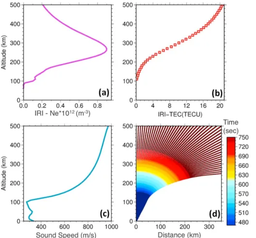
We emphasize that both these methods will significantly rely on the altitude of CID detection (Hion) in the GNSS-sounding method. Hion cannot be known for certain but can be suggested from physical principles. It is known that TEC is an integral parameter equal to the total number of electrons along a line of sight between a satellite and a receiver. It is generally assumed that the TEC perturbations are concentrated around the alti-tude of the maximum ionosphere ionization, that is, in the ionospheric F layer. To track the TEC perturbations, the ionosphere is considered as a thin shell layer at the altitude Hion, so that the intersection points between a line of sight and the thin ionospheric shell that are called ionospheric piercing points (IPPs) will provide the coordinates of observed TEC disturbances. Changing the Hion will change the IPP coordinates, and therefore, the choice of the Hion is extremely important for the ionospheric imagery of the seismic source (Astafyeva, Rolland, et al., 2013). Some hints on the altitude of detection can be found from 3-D analysis of the GNSS-sounding geometry, including elevation angles of detection (Thomas et al., 2018). Also, comparison of the real CID arrival times with the theoretic arrival times of the acoustic waves at different altitudes may help. For the 2011 Sanriku-oki earthquake, by using only data of satellite G07 Thomas et al. (2018) found extre-mely earlyfirst CID arrivals and explained them by a particular geometry of sounding at low-elevation angles. Thomas et al. (2018) found that thefirst ionospheric detection took place at around 130 km of alti-tude, which is much below the ionization maximum of 275 km as follows from the International Reference Ionosphere (IRI) model (Bilitza et al., 2017; Figure 3a). Our results here confirm that for both G07 and G10 measurements the first CID occur 470–480 s after the earthquake (Figures 1b–1d).
Figure 3. (a) Ionospheric electron density profile as deduced from the online IRI-2016 model (https://ccmc.gsfc.nasa.gov/ modelweb/models/iri2016_vitmo.php) for the date, time, and location of the Sanriku-oki earthquake. (b) Absolute vertical total electron content (TEC) from the ground up to the altitude on Y axis as derived from the online IRI-2016 model. (c) Sound speed profile calculated for the atmospheric conditions of 9 March 2011 by using the empirical atmosphere model NRLMSISE-00 (Picone et al., 2002). (d) Acoustic ray-tracing for incidence angles 0 to 24° using the sound speed profile shown in panel (c). The propagation time along the rays is marked in color with a particular focus on the range 470–750 s (the color scale is shown on the right).
10.1029/2018JA026107
Considering the vertical velocity of acoustic waves, the perturbations were, most likely, indeed, detected at altitudes much lower than 275 km. Simple acoustic ray-tracing (method similar to Heki & Ping, 2005) for atmospheric conditions of 9 March 2011 (the sound speed profile presented in Figure 3c) shows that in a time period of 470–480 s, the acoustic waves above the source area will only reach the altitudes of ~140– 150 km (Figure 3d). However, at these altitudes the background electron density is quite low (Figure 3a) and the background absolute TEC below this altitude reaches only 0.5–0.7 TECU (Figure 3b). Therefore, it might be doubtful that CID of any discernible amplitude can be generated at such low ionospheric background. It should be noted that thefirst CID arrival is the time when the CID only starts to develop, and the CID is formed at the point of the TEC maximum. By the time of thefirst maximums at ~510–520 s (Figures 1b–1d), the acoustic waves will reach 180–200 km (Figure 3d), with the background TEC of about 1.4–2.2 TECU (Figure 3b). With the maximum amplitude of thefirst detected CID of ~0.04–0.08 TECU (Figures 1b–1d), the CID then represents ~4–5% of the background, which is more credible but yet might be questionable. In addition to the above conceptions on the theoretic arrivals of the acoustic waves and the background ioni-zation, we can investigate how changing the altitude of CID detection will change the positions of the IPP for the Sanriku-oki case. Figures 4a–4c show the location of the first arrivals (which normally would show the location of the seismic source) at 480 s after the earthquake depending on Hion. Here we analyze the CID position for Hion located at the ionization maximum of 275 km (a), at 140 km where we seem to detect thefirst arrivals (b) and at 190 km where we detect the first TEC maximums (c). One can see that for
Hion= 275 km thefirst CID is located far away from the epicentral area, while for Hion = 140 km the first TEC perturbation is detected closer to the epicenter, but on the southwest from it. The best agreement between the source and the CID is reached for Hion=180–190 km (Figure 4c).
3.3. Acoustic and Shock-Acoustic Waves
Let us now recall that CIDs are often referred to as shock-acoustic waves rather than regular acoustic waves (e.g., Afraimovich et al., 2001, 2006; Astafyeva, Shalimov, et al., 2013; Blanc, 1985). This presumes that in the atmosphere the acoustic waves become shock-acoustic and may propagate at speeds exceeding the sound speed and, consequently, reach higher altitudes faster. The difference in the wave speed between the acous-tic and shock waves will appear starting from ~100 to 120 km of altitude and will depend on the Mach num-ber (M). Thus, for M = 1 at ~190 km the shock waves will be several seconds ahead of the acoustic waves (Besset & Blanc, 1994), while faster shock waves can gain several tens of seconds with respect to the acoustic waves (Daniels et al., 1960). The difference in propagation time between the two types of wave increases with altitude and at 300–400 km may reach 2–3 min. We note however that all this primarily concerns strong atmospheric sources such as explosions or underground nuclear explosions. Besides atmospheric sources, giant shallow earthquakes such as the 2011 Tohoku-oki earthquake can also produce shock waves as recently has been shown by observations and modeling (e.g., Astafyeva et al., 2011; Zettergren et al.,
Figure 4. Snapshots of total electron content (TEC) measurements at 480 s after the earthquake for the altitude Hion of (a) 275 km, (b) 140 km, and (c) 190 km. Each colored point corresponds to an ionospheric piercing point between a satellite and a receiver at Hion, the color indicates the TEC value, and the corresponding color scale is shown on the right. The red star shows the epicenter magenta cross- the co-seismic vertical uplift.
2017). Whereas, transformation of the acoustic waves into shock-acoustic waves for smaller amplitude earthquakes seems yet debatable.
Concerning our results on the Sanriku-oki earthquake, its moment magnitude was only 7.4, but several of our observations are difficult to explain in terms of regular acoustic waves: (1) early CID arrivals presume that the CID were detected at very low altitudes where the background TEC might be too low to produce discernible TEC perturbations; (2) from traveltime diagrams, the apparent horizontal velocities of 1.1 and 1.3 km/s exceed or largely exceed the sound speed at ionospheric altitudes, especially if the altitude of detec-tion is low (Figure 3c); (3) the horizontal distances traveled by the CID as seen in our observadetec-tions are also difficult to explain. Figures 5a–5c show TEC snapshots for Hion = 190 km and time moments 600 s (a), 650 s (b), and 700 s (c) after the earthquakes. Comparison of the horizontal distances traveled with time by theo-retic acoustic waves (Figure 3d) and those passed by real CID (Figures 5a–5c) reveals that CID generated by the Sanriku-oki earthquake traveled faster than the theoretic acoustic waves. The latter two observations can be partly explained by discrepancies in our assumptions and the real CID propagation. For instance, the fact that in reality CID propagate upward with time, whereas, for the GNSS-sounding, we use the constant alti-tude Hion for all observations, from thefirst CID detection to later observations.
Current results are a good demonstration that our understanding and knowledge of the CID origin and evo-lution are yet not quite sufficient, and they also present challenges for future works.
3.4. CID Formation Over the Epicentral Area: Ionospheric Imagery of the Seismic Source
Let us now analyze in detail the formation of CID over the epicentral area and its further evolution. Animation S1 in the supporting information shows the TEC variations around the epicentral area of the Sanriku-oki earthquake from the moment of the earthquake at 02:45:20UT until 900 s after it. One can see that within thefirst ~470 s after the earthquake onset the TEC varied within ±0.05 TECU, which is in the range of the background TEC variations. Starting from 470 s, the TEC on the east-northeast from the epicenter exceeds the background level, so that we can affirm reliable detection of a CID. We emphasize that this area of the first enhanced TEC corresponds to the uplift area as was estimated by Thomas et al. (2018) and as shown by white cross in Figure 1a. Thisfirst CID seems to further move southward while simultaneously extending westward. At this time, the CID amplitude increases up to 0.15–0.20 TECU. From ~555 s, we observe a small depletion over the area of the initial TEC increase. This TEC depletion is, most likely, the representation of the negative half-phase of the N-wave (Astafyeva, Shalimov, et al., 2013) and is often observed over the epicentral regions (e.g., Kakinami et al., 2012). From this source region both positive and negative half-phases further propagate south-westward and intensify. Starting from ~710 s after the earthquake onset, the positive phase of the CID seemed to fade, while the negative phase continued for about 200 s more.
Overall, several importantfindings can be retrieved from the TEC snapshots presented in Animation S1: first, and foremost, the position of the first CID arrivals corresponds to the position of the coseismic uplift on the north-northeast from the epicenter. Second, the dimensions of the ionospheric source region roughly correspond to the area of the coseismic uplift occurred due to the earthquake. Note that the Sanriku-oki
Figure 5. Snapshots of total electron content (TEC) measurements at the altitude Hion = 190 km taken at (a) 600 s, (b) 650 s, and (c) 700 s after the earthquake. Each colored point corresponds to an ionospheric piercing point between a satellite and a receiver at Hion, the color indicates the TEC value, and the corresponding color scale is shown on the right. The red star shows the epicenter. The circles indicate 50-, 100-, 200-, and 300-km distance from the epicenter.
10.1029/2018JA026107
earthquake is an example of a large but not giant earthquake, and it was characterized by rather simple seis-mic fault zone that contained only one segment of uplift with dimensions ~45 * 40 km. For larger and much larger earthquakes, the fault is usually much more complex: it is extended and often comprises several seg-ments (subuplifts). The structure of a seismic source can be understood from seismological data, but also, as recent seismo-ionospheric results suggest, it can be done from ionospheric TEC measurements. For instance, in the case of the great M9.1 2004 Sumatra earthquake, the seismic fault was elongated for nearly ~1,300 km and consisted of six segments. Heki et al. (2006) from ionospheric GPS data managed to reconstruct the rup-ture process, showing contribution of each of the six segments in the observed CID. In the case of the Tohoku-oki earthquake, the source with dimensions ~350 * 150 km was located ~120–150 km eastward from the epicenter. Seismological data sets showed that the source region consisted of two main segments (Bletery et al., 2014; Simons et al., 2011), and Astafyeva, Rolland, et al. (2013) showed the same by using ionospheric 1-Hz TEC data. These examples, along with our current results, demonstrate that ionospheric TEC data can help with the reconstruction of the seismic source parameters from the ionosphere shortly after an earth-quake, provided that the geometry of GNSS sounding is fortunate and the Hion is determined. Our results, therefore, could be used in the future for near–real-time ionosphere-based tsunami warning systems for smaller and giant earthquakes. It should be noted, however, that ionospheric imagery of seismic source is only possible while using high-rate ionospheric data. Standard data sampling for GNSS of 30 s or 10–15 s might not provide the desired results because of low resolution. For instance, we attempted to obtain images for the M7.8 2015 Nepal earthquake by using standard 30-s GPS data but we failed.
4. Conclusions
In this work, by using 1-Hz data from ground-based GPS receivers of the GEONET, we analyzed the iono-spheric response to the Mw7.4 Sanriku-oki earthquake of 9 March 2011. Two GPS satellites, G07 and G10, sounded the epicentral area and showed the occurrence of TEC enhancement on the east-northeast from the epicenter starting from 470– 480 s (~7.8–8 min) after the earthquake. The location of this initial TEC increase corresponds to the location of the coseismic crustal uplift that occurred due to the earthquake. The main difficulty of the method of the GNSS-based ionospheric imagery lies in an unknown altitude of ionospheric detection Hion. Here we showed that knowing the real time of thefirst CID arrivals together with the theoretic arrival time of the acoustic waves helps to overcome this difficulty. Overall, our results confirm that despite several difficulties, high-rate ionospheric GPS data can be used for determining the seis-mic source parameters from the ionosphere. This method should work for both giant and smaller/moderate earthquakes.
Finally, our observations raise several fundamental questions, merely, on the acoustic or shock-acoustic nat-ure of CID generated by smaller earthquakes. Can moderate earthquake generate shock waves?—this ques-tion is yet to answer.
References
Afraimovich, E., Feng, D., Kiryushkin, V., & Astafyeva, E. (2010). Near-field TEC response to the main shock of the 2008 Wenchuan earthquake. Earth, Planets and Space, 62(11), 899–904. https://doi.org/10.5047/eps.2009.07.002
Afraimovich, E. L., Astafieva, E. I., & Kirushkin, V. V. (2006). Localization of the source of ionospheric disturbance generated during an earthquake. International Journal of Geomagnetism and Aeronomy, 6, GI2002. https://doi.org/10.1029/200403000092
Afraimovich, E. L., Perevalova, N. P., Plotnikov, A. V., & Uralov, A. M. (2001). The shock-acoustic waves generated by the earthquakes.
Annales de Geophysique, 19(4), 395–409. https://doi.org/10.5194/angeo-19-395-2001
Astafyeva, E., & Heki, K. (2009). Dependence of waveform of near-field coseismic ionospheric disturbances on focal mechanisms. Earth,
Planets and Space, 61(7), 939–943. https://doi.org/10.1186/BF03353206
Astafyeva, E., Heki, K., Afraimovich, E., Kiryushkin, V., & Shalimov, S. (2009). Two-mode long-distance propagation of coseismic iono-sphere disturbances. Journal of Geophysical Research, 114, A10307. https://doi.org/10.1029/2008JA013853
Astafyeva, E., Lognonné, P., & Rolland, L. (2011). First ionosphere images for the seismic slip on the example of the Tohoku-oki earth-quake. Geophysical Research Letters, 38, L22104. https://doi.org/10.1029/2011GL049623
Astafyeva, E., Rolland, L., Lognonné, P., Khelfi, K., & Yahagi, T. (2013). Parameters of seismic source as deduced from 1 Hz ionospheric GPS data: Case-study of the 2011 Tohoku-oki event. Journal of Geophysical Research: Space Physics, 118, 5942–5950. https://doi.org/ 10.1002/jgra50556
Astafyeva, E., Rolland, L., & Sladen, A. (2014). Strike-slip earthquakes can also be seen in the ionosphere. Earth and Planetary Science
Letters, 405, 180–193. https://doi.org/10.1016/j.epsl.2014.08.024
Astafyeva, E., Shalimov, S., Olshanskaya, E., & Lognonné, P. (2013). Ionospheric response to earthquakes of different magnitudes: Larger quakes perturb the ionosphere stronger and longer. Geophysical Research Letters, 40, 1675–1681. https://doi.org/10.1002/ grl.50398
Acknowledgments
This work was supported by the European Research Council (ERC, grant agreement 307998). We thank the Geospatial Information Authority of Japan (GSI) for the GEONET RINEX data (ftp://terras.gsi.go.jp/) and the CCMC web-services (https://ccmc.gsfc. nasa.gov/modelweb/models/iri2016_ vitmo.php) for the online runs of the IRI-2016 model. The authors thank Kosuke Heki (Hokkaido University) for the initial version of the RayTracing codes. Discussions with Mala S. Bagiya (Indian Institute of Geomagnetism) and Jonathan Snively (Embry-Riddle Aeronautical University) were useful. Thefigures were made by using the Generic Mapping Tools (GMT; Wessel & Smith, 1998). This is IPGP contribu-tion 4000.
Bagiya, M. S., Sunil, A. S., Sunil, P. S., Sreejith, K. M., Rolland, L., & Ramesh, D. S. (2017). Efficiency of coseismic ionospheric perturbations in identifying crustal deformation pattern: Case study based on Mw7.3 May Nepal 2015 earthquake. Journal of Geophysical Research:
Space Physics, 122, 6849–6857. https://doi.org/10.1002/2017JA024050
Bagiya, M. S., Sunil, P. S., Sunil, A. S., & Ramesh, D. S. (2018). Coseismic contortion and coupled nocturnal ionospheric perturbations during 2016 Kaikoura, Mw7.8 New Zealand earthquake. Journal of Geophysical Research: Space Physics, 123, 1477–1487. https://doi.org/ 10.1002/2017JA024584
Besset, C., & Blanc, E. (1994). Propagation of vertical shock waves in the atmosphere. The Journal of the Acoustical Society of America, 95(4), 1830–1839. https://doi.org/10.11121/1.408689
Bilitza, D., Altadill, D., Truhlik, V., Shubin, V., Galkin, I., Reinisch, B., & Huang, X. (2017). International Reference Ionosphere 2016: From ionospheric climate to real-time weather predictions. Space Weather, 15, 418–429. https://doi.org/10.1002/ 2016SW001593
Blanc, E. (1985). Observations in the upper atmosphere of infrasonic waves from natural or artificial sources—A summary. Annales de
Geophysique, 3, 673–687.
Bletery, Q., Sladen, A., Delouis, B., Vallée, M., Nocquet, J.-M., Rolland, L., & Jiang, J. (2014). A detailed source model for the Mw9.0 Tohoku-Oki earthquake reconciling geodesy, seismology and tsunami records. Journal of Geophysical Research: Solid Earth, 119, 7636–7653. https://doi.org/10.1002/2014JB011261
Calais, E., & Minster, J. B. (1995). GPS detection of ionospheric perturbations following the January 17, 1994, Northridge earthquake.
Geophysical Research Letters, 22, 1045–1048. https://doi.org/10.1029/95GL00168
Daniels, F. B., Bauer, S. J., & Harris, A. K. (1960). Vertically travelling shock waves in the ionosphere. Journal of Geophysical Research, 65, 1848–1850. https://doi.org/10.1029/JZ065i006p01848
Ducic, V., Artru, J., & Lognonne, P. (2003). Ionospheric remote sensing of the Denali earthquake Rayleigh surface waves. Geophysical
Research Letters, 30(18), 1951. https://doi.org/10.1029/2003GL017812
Heki, K., Otsuka, Y., Choosakul, N., Hemmakorn, N., Komolmis, T., & Maruyama, T. (2006). Detection of ruptures of Andaman fault segments in the 2004 great Sumatra earthquake with coseismic ionospheric disturbances. Journal of Geophysical Research, 111, B09313. https://doi.org/10.1029/2005JB004202
Heki, K., & Ping, J. (2005). Directivity and apparent velocity of the coseismic ionospheric disturbances observed with a dense GPS array.
Earth and Planetary Science Letters, 236, 845–855.
Hofmann-Wellenhof, B., Lichtenegger, H., & Wasle, E. (2008). GNSS—Global Navigation Satellite Systems. Vienna: Springer. https://doi. org/10.1007/978-3-211-73017-1
Jakowski, N., Wilken, V., Tsybulya, K., & Heise, S. (2006). Earthquake signatures in the ionosphere deduced from ground and space based GPS measurements. Observation of the Earth System from Space, 43–53. https://doi.org/10.1007/3-540-29522-4_4
Jin, S., Zhu, W., & Afraimovich, E. (2010). Co-seismic ionospheric and deformation signals on the 2008 magnitude 8.0 Wenchuan Earthquake from GPS observations. International Journal of Remote Sensing, 31(13), 3535–3543. https://doi.org/10.1080/ 01431161003727739
Kakinami, Y., Kamogawa, M., Tanioka, Y., Watanabe, S., Gusman, A. R., Liu, J.-Y., et al. (2012). Tsunamigenic ionospheric hole.
Geophysical Research Letters, 39, L00G27. https://doi.org/10.1029/2011GL050159
Kamogawa, M., Orihara, Y., Tsurudome, C., Tomida, Y., Kanaya, T., Ikeda, D., et al. (2016). A possible space-based tsunami early warning system using observations of the tsunami ionospheric hole. Scientific Reports, 6(1), 37989. https://doi.org/10.1038/srep37989 Klobuchar, J. A. (1986). Ionospheric time-delay algorithmfor single frequency GPS users. IEEE Transactions on Aerospace and Electronic
Systems AES, 23(3), 325–331.
Komjathy, A., Yang, Y.-M., Meng, X., Verkhoglyadova, O., Mannucci, A. J., & Langley, R. B. (2016). Review and perspectives: Understanding natural-hazards-generated ionospheric perturbations using GPS measurements and coupled modeling. Radio Science,
51, 951–961. https://doi.org/10.1002/2015RS005910
Lee, R. F., Rolland, L. M., & Mykesell, T. D. (2018). Seismo-ionospheric observations, modeling and backprojection of the 2016 Kaikoura earthquake. Bulletin of the Seismological Society of America, 108(3B), 1794–1806. https://doi.org/10.1785/0120170299
Liu, J. Y., Chen, C. H., Lin, C. H., Tsai, H. F., Chen, C. H., & Kamogawa, M. (2011). Ionospheric disturbances triggered by the 11 March 2011 M9.0 Tohoku earthquake. Journal of Geophysical Research, 116, A06319. https://doi.org/10.1029/2011JA016761
Liu, J. Y., Tsai, H. F., Lin, C. H., Kamogawa, M., Chen, Y. I., Lin, C. H., et al. (2010). Coseismic ionospheric disturbances triggered by the Chi-Chi earthquake. Journal of Geophysical Research, 115, A08303. https://doi.org/10.1029/2009JA014943
Perevalova, N. P., Sankov, V. A., Astafyeva, E. I., & Zhupityaeva, A. S. (2014). Threshold magnitude for ionospheric response to earth-quakes. Journal of Atmospheric and Solar - Terrestrial Physics, 108, 77–90. https://doi.org/10.1016/j.jastp.2013.12.014
Picone, J., Hedin, A., Drob, D., & Aikin, A. (2002). NRLMSISE-00 empirical model of the atmosphere: Statistical comparisons and scientific issues. Journal of Geophysical Research, 107(A12), 1468. https://doi.org/10.1029/2002JA009430
Reddy, C. D., & Seemala, G. K. (2015). Two-mode ionospheric response and Rayleigh wave group velocity distribution reckoned from GPS measurement following Mw 7.8 Nepal earthquake on 25 April 2015. Journal of Geophysical Research: Space Physics, 120, 7049–7059. https://doi.org/10.1002/2015JA021502
Rolland, L., Lognonné, P., Astafyeva, E., Kherani, A., Kobayashi, N., Mann, M., & Munekane, H. (2011). The resonant response of the ionosphere imaged after the 2011 Tohoku-oki earthquake. Earth, Planets and Space, 63(7), 853–857. https://doi.org/10.5047/ eps.2011.06.020
Rolland, L. M., Vergnolle, M., Nocquet, J.-M., Sladen, A., Dessa, J.-X., Tavakoli, F., et al. (2013). Discriminating the tectonic and non-tectonic contributions in the ionospheric signature of the 2011, Mw7.1, dip-slip Van earthquake, eastern Turkey. Geophysical Research
Letters, 40, 2518–2522. https://doi.org/10.1002/grl.50544
Savastano, G., Komjathy, A., Verkhoglyadova, O., Mazzoni, A., Crespi, M., Wei, Y., & Mannucci, A. J. (2017). Real-time detection of tsu-nami ionospheric disturbances with a stand-alone GNSS-receiver: A preliminary feasibility demonstration. Scientific Reports, 7, 46607. https://doi.org/10.1038/srep46607
Shao, G., Ji, C., & Zhao, D. (2011). Rupture process of the 9 March, 2011 Mw 7.4 Sanriku-Oki, Japan earthquake constrained by jointly inverting teleseismic waveforms, strong motion data and GPS observations. Geophysical Research Letters, 38, L00G20. https://doi.org/ 10.1029/2011GL049164
Shults, K., Astafyeva, E., & Adourian, S. (2016). Ionospheric detection and localization of volcano eruptions on the example of the April 2015 Calbuco events. Journal of Geophysical Research: Space Physics, 121, 10,303–10,315. https://doi.org/10.1002/2016JA023382 Simons, M., Minson, S. E., Sladen, A., Ortega, F., Jiang, J., Owen, S. E., et al. (2011). The 2011 magnitude 9.0 Tohoku-oki earthquake:
Mosaicking the megathrust from seconds to centuries. Science, 332(6036), 1421–1425. https://doi.org/10.1126/science.1206731
10.1029/2018JA026107
Thomas, D., Bagiya, M. S., Sunil, P. S., Rolland, L., Sunil, A. S., Mikesell, T. D., et al. (2018). Revelation of early detection of co- seismic ionospheric perturbations in GPS-TEC from realistic modelling approach: Case study. Scientific Reports, 8(1), 12105. https://doi.org/ 10.1038/s41598-018-30476-9
Wessel, P., & Smith, W. H. F. (1998). New, improved version of the Generic Mapping Tools released. Eos, Transactions American
Geophysical Union, 79(47), 579. https://doi.org/10.1029/98EO00426
Zettergren, M., & Snively, J. B. (2015). Ionospheric response to infrasonic-acoustic waves generated by natural hazard events. Journal of
Geophysical Research: Space Physics, 120, 8002–8024. https://doi.org/10.1002/2015JA021116
Zettergren, M. D., Snively, J. B., Komjathy, A., & Verkhoglyadova, O. P. (2017). Nonlinear ionospheric responses to large-amplitude infrasonic-acoustic waves generated by undersea earthquakes. Journal of Geophysical Research: Space Physics, 122, 2272–2291. https:// doi.org/10.1002/2016JA023159