Characterization of Cortical Networks and Corticocortical Functional Connectivity Mediating Arbitrary Visuomotor Mapping

HAL Id: hal-02087533

https://hal-amu.archives-ouvertes.fr/hal-02087533

Submitted on 2 Apr 2019

HAL is a multi-disciplinary open access

archive for the deposit and dissemination of

sci-entific research documents, whether they are

pub-lished or not. The documents may come from

teaching and research institutions in France or

abroad, or from public or private research centers.

L’archive ouverte pluridisciplinaire HAL, est

destinée au dépôt et à la diffusion de documents

scientifiques de niveau recherche, publiés ou non,

émanant des établissements d’enseignement et de

recherche français ou étrangers, des laboratoires

publics ou privés.

Corticocortical Functional Connectivity Mediating

Arbitrary Visuomotor Mapping

Andrea Brovelli, Daniel Chicharro, Jean-Michel Badier, Huifang Wang, Viktor

Jirsa

To cite this version:

Andrea Brovelli, Daniel Chicharro, Jean-Michel Badier, Huifang Wang, Viktor Jirsa.

Characteriza-tion of Cortical Networks and Corticocortical FuncCharacteriza-tional Connectivity Mediating Arbitrary

Visuomo-tor Mapping. Journal of Neuroscience, Society for Neuroscience, 2015,

�10.1523/JNEUROSCI.4892-14.2015�. �hal-02087533�

Behavioral/Cognitive

Characterization of Cortical Networks and Corticocortical

Functional Connectivity Mediating Arbitrary Visuomotor

Mapping

X

Andrea Brovelli,

_{Daniel Chicharro,}

_{Jean-Michel Badier,}

_{Huifang Wang,}

_{and Viktor Jirsa}

1_{Institut de Neurosciences de la Timone UMR 7289, Aix Marseille Universite´, CNRS, 13385 Marseille, France,}2_{Neural Computation Laboratory, Center for}

Neuroscience and Cognitive Systems@UniTn, Istituto Italiano di Tecnologia, Rovereto, Italy,3_{Aix Marseille Universite´, INS UMR S1106, 13005 Marseille,}

France, and4_{Inserm, UMR S1106, 13005 Marseille, France}

Adaptive behaviors are built on the arbitrary linkage of sensory inputs to actions and goals. Although the sensorimotor and associative

frontostriatal circuits are known to mediate arbitrary visuomotor mappings, the underlying corticocortico dynamics remain elusive.

Here, we take a novel approach exploiting gamma-band neural activity to study the human cortical networks and corticocortical

func-tional connectivity mediating arbitrary visuomotor mapping. Single-trial gamma-power time courses were estimated for all Brodmann

areas by combing magnetoencephalographic and MRI data with spectral analysis and beam-forming techniques. Linear correlation and

Granger causality analyses were performed to investigate functional connectivity between cortical regions. The performance of

visuo-motor associations was characterized by an increase in gamma-power and functional connectivity over the sensorivisuo-motor and

frontopa-rietal network, in addition to medial prefrontal areas. The superior pafrontopa-rietal area played a driving role in the network, exerting Granger

causality on the dorsal premotor area. Premotor areas acted as relay from parietal to medial prefrontal cortices, which played a receiving

role in the network. Link community analysis further revealed that visuomotor mappings reflect the coordination of multiple

subnet-works with strong overlap over motor and frontoparietal areas. We put forward an associative account of the underlying cognitive

processes and corticocortical functional connectivity. Overall, our approach and results provide novel perspectives toward a better

understanding of how distributed brain activity coordinates adaptive behaviors.

Key words: corticocortical coupling; functional connectivity; gamma-band neural activity; Granger causality;

magnetoencephaplogra-phy; visuomotor behaviors

Introduction

Most cognitive functions arise from the dynamic coordination of

neural activity distributed over large-scale brain networks (

Bressler

and Menon, 2010

). Adaptive behaviors and the ability to flexibly

choose appropriate actions depending on visual cues and internal

goals are no exceptions. A key form of visuomotor guidance is the

Received Dec. 1, 2014; revised July 7, 2015; accepted July 22, 2015.

Author contributions: A.B. designed research; A.B. and J.-M.B. performed research; A.B., D.C., H.W., and V.J. contributed unpublished reagents/analytic tools; A.B. analyzed data; A.B., D.C., H.W., and V.J. wrote the paper.

This work was supported by Projets exploratoires pluridisciplinaires from the CNRS/Inserm/Inria “Bio-math-Info” entitled “Computational and neurophysiological bases of goal-directed and habit learning.” D.C. was supported by the Autonomous Province of Trento, Call “Grandi Progetti 2012” project “Characterizing and improving brain mech-anisms of attention—ATTEND”. V.J. was supported by FP7 BrainScaleS and the James S. McDonell Foundation. We

thank Faical Isbaine and Sophie Chen for helping in the MEG experiments; and Driss Boussaoud and Pascal Huguet for useful discussion.

The authors declare no competing financial interests.

Correspondence should be addressed to Dr. Andrea Brovelli, Institut de Neurosciences de la Timone, UMR 7289 CNRS, Aix Marseille University, Campus de Sante´ Timone, 27 Bd Jean Moulin, 13385 Marseille, France. E-mail: andrea.brovelli@univ-amu.fr.

DOI:10.1523/JNEUROSCI.4892-14.2015

Copyright © 2015 the authors 0270-6474/15/3512643-16$15.00/0

Significance Statement

In everyday life, most of our behaviors are based on the arbitrary linkage of sensory information to actions and goals, such as

stopping at a red traffic light. Despite their automaticity, such behaviors rely on the activity of a large brain network and elusive

interareal functional connectivity. We take a novel approach exploiting noninvasive recordings of human brain activity to reveal

the cortical networks and corticocortical functional connectivity mediating visuomotor mappings. Parietal areas were found to

play a driving role in the network, whereas premotor areas acted as relays from parietal to medial prefrontal cortices, which played

a receiving role. Overall, our approach and results provide novel perspectives toward a better understanding of how distributed

brain activity coordinates adaptive behaviors.

ability to learn arbitrary and causal relations linking visual inputs to

actions and outcomes, named arbitrary visuomotor learning (

Wise

and Murray, 2000

). Performance of arbitrary visuomotor mappings

relies on the neural activity of the associative and sensorimotor

fron-tostriatal circuits (

Wise et al., 1996

;

Murray et al., 2000

;

Passingham

et al., 2000

;

Wise and Murray, 2000

;

Hadj-Bouziane et al., 2003

;

Petrides, 2005

). However, the interplay between these brain regions

is still unclear.

A potential key player for uncovering functional cortical

net-works is the gamma-band (30 –150 Hz) neural activity. Animal

studies have observed narrow-band low-gamma oscillations in

the 30 – 80 Hz range during sensory stimulation (

Ray and

Maun-sell, 2010

) and cognitive processes, such as attention (

Fries et al.,

2001

;

Bichot et al., 2005

;

Buschman and Miller, 2007

;

Gregoriou

et al., 2009

;

Bosman et al., 2012

) and working memory (

Pesaran

et al., 2002

). Human studies have consistently found correlates of

cognitive processes in the high-gamma range (from 60 to 150 Hz)

in invasive (

Brovelli et al., 2005

;

Crone et al., 2006

;

Jerbi et al.,

2009

;

Lachaux et al., 2012

;

Cheyne and Ferrari, 2013

;

Ko et al.,

2013

), noninvasive (

Vidal et al., 2006

;

Ball et al., 2008

;

Darvas et

al., 2010

), and multimodal neurophysiological studies (

Dalal et

al., 2009

). Correlations with BOLD responses in animals (

Logo-thetis et al., 2001

;

Niessing et al., 2005

;

Goense and Logothetis,

2008

) and humans (

Lachaux et al., 2007

;

Nir et al., 2007

;

Scheer-inga et al., 2011

;

Hermes et al., 2012

;

Ojemann et al., 2013

) further

suggest gamma-band activity as a proxy for local processing.

At the large-scale level, binding local activations into

coordi-nated spatiotemporal network activity results from a complex

interplay between neuronal dynamics and anatomical

connectiv-ity. To quantify the degree of coordination, functional

connec-tivity (FC) measures include various forms of statistical

dependences between neural signals, such as linear correlation

and Granger causality (

Brovelli et al., 2004

;

Ding et al., 2006

;

Bressler and Seth, 2011

). Patterns of FC can then be analyzed

through network-based measures using graph theory (

Rubinov

and Sporns, 2010

). Here, we take a novel approach based on

gamma-band neural activity and FC analysis to reveal the human

cortical networks and FC mediating arbitrary visuomotor

map-ping. Single-trial gamma-power time courses were estimated for

all Brodmann areas (BAs) by combining

magnetoencephalo-graphic (MEG) and structural MRI data with spectral analysis

and beam-forming techniques. Performance of visuomotor

asso-ciations was characterized by an increase in high-gamma activity

(HGA) and FC over the sensorimotor and frontoparietal network

together with medial prefrontal areas. Graph measures and link

community analysis (

Ahn et al., 2010

) further support that

arbi-trary visuomotor mappings are mediated by overlapping cortical

subnetworks dominated by a core circuit, exchanging Granger

interdependences, centered over the dorsal frontoparietal

network, with a privileged role for the premotor and medial

prefrontal areas.

Materials and Methods

Experimental procedure and data acquisition

Experimental conditions and behavioral tasks. Eleven healthy participants

accepted to take part in our study (all were right handed; the average age was⬃23 years; 4 were females and 7 males), gave written informed consent according to established institutional guidelines and local ethics committee, and received monetary compensation (€50). We used an associative visuomotor mapping task, where the relation between visual stimulus and motor response is arbitrary and deterministic (Wise and Murray, 2000). The domain of visuomotor control distinguishes two forms of guidance: standard and nonstandard (or arbitrary) mapping. In standard mapping, such as reaching toward an object, the spatial

prop-erties of the visual cue (i.e., target location) provide relevant information for visuomotor transformation. In arbitrary mapping, the visual cue and the action are not spatially congruent; and other properties of the object, such as its form or color, are transformed to plan actions (Petrides, 1987;

Wise et al., 1996;Murray et al., 2000;Passingham et al., 2000;Wise and Murray, 2000). To investigate arbitrary visuomotor mapping, we asked participants to perform a finger movement associated to a digit number: digit 1 instructed the execution of the thumb, digit 2 for the index finger, digit 3 for the middle finger, and so on (Fig. 1). Maximal reaction time was 1 s. After a fixed delay of 1 s following the disappearance of the digit number, an outcome image was presented for 1 s and informed the subject whether the response was correct, incorrect, or too late (if the reaction time exceeded 1 s). Incorrect and late trials were excluded from the analysis because they were either absent or very rare (i.e., maximum 2 late trials per session). The next trial started after a variable delay ranging from 2 to 3 s (randomly drawn from a uniform distribution) with the presentation of another visual stimulus (Fig. 1b). Each

partici-pant performed two sessions of 60 trials each (total of 120 trials). Each session included three digits randomly presented in blocks of three trials.

Anatomical, functional, and behavioral data acquisition. Anatomical

MRI images were acquired for each participant using a 3-T whole-body imager equipped with a circular polarized head coil. High-resolution structural T1-weighted anatomical image (inversion-recovery sequence, 1⫻ 0.75 ⫻ 1.22 mm) parallel to the anterior commissure-posterior commissure plane, covering the whole brain, were acquired. MEG re-cordings were performed using a 248 magnetometers system (4D Neu-roimaging, magnes 3600). Visual stimuli were projected using a video projection, and motor responses were acquired using a LUMItouch op-tical response keypad with five keys. Presentation software was used for stimulus delivery and experimental control during MEG acquisition. Reaction times were computed as the time difference between stimulus onset and motor response. Sampling rate was 2034.5 Hz. Location of the participant’s head with respect to the MEG sensors was recorded both at the beginning and end of each session to potentially exclude sessions and/or participants with large head movements. However, none of the participants moved⬎3 mm during all sessions. Thus, all participants were considered for further analysis.

Single-trial HGA at BAs

Preprocessing and spectral analysis of MEG signals. MEG signals were

down-sampled to 1 kHz, low-pass filtered to 250 Hz, and segmented into epochs aligned on finger movement (i.e., button press). Epoch segmen-tation was also performed on stimulus onset and the data from⫺0.5 and ⫺0.1 s before stimulus presentation was taken as baseline activity for the

NO

1

a

b

Figure 1. Arbitrary visuomotor mapping task. a, The relation between visual stimulus and motor response is deterministic and highly acquainted. Stimuli were digits from 1 to 5 and appeared at the center of the screen for 1 s. Participants were required to move the finger associated to the digit: 1, instructed thumb movement; 2, the index, etc. b, The maximum reaction time was 1 s (i.e., stimulus duration). After a fixed delay of 1 s, the feedback image instructed whether the executed motor response was correct, incorrect, or late.

calculation of the single-trial HGA. Artifact rejection was performed semiautomatically. For each movement-aligned epoch and channel, the MEG signal variance and z-value were computed over time and taken as relevant metrics for the identification of artifact epochs. All trials with a variance⬎1.5 ⫻ 10⫺24across channels were excluded from further anal-yses. Additional metrics, such as the z-score, absolute z-score, and range between the minimum and maximum values, were also inspected to detect artifact. Two MEG sensors were excluded from the analysis for all subjects.

Spectral density estimation was performed using a multitaper method based on discrete prolate spheroidal (slepian) sequences (Percival and Walden, 1993;Mitra and Pesaran, 1999). To define the frequency band-width of interest for the estimate of single-trial gamma-band activity, we performed time-frequency analyses of the MEG time series at the sensor level. MEG fields were transformed to a planar gradient configuration (i.e., by computing the gradient tangential to the scalp). Time-frequency power estimates were then computed for all sensors over the gamma band from 30 to 150 Hz (in steps of 5 Hz) using 4 orthogonal tapers 0.25 s in duration and 20 Hz of frequency resolution, each stepped every 0.01 s. Time-frequency power estimates were log-transformed and then nor-malized (i.e., z-transformed) with respect to the mean and SD computed over a baseline period from⫺0.5 to ⫺0.1 s before stimulus onset. Time-frequency maps were averaged across virtual gradiometers and partici-pants. Results showed increases in power with respect to baseline in the high-gamma range from⬃60 to 120 Hz (Fig. 2). Based on the spectral analysis at the sensors level, subsequent analyses focused on the high-gamma band from 60 to 120 Hz. MEG time series were multiplied by k orthogonal tapers (k⫽ 8) (0.15 s in duration and 60 Hz of frequency resolution, each stepped every 0.005 s), centered at 90 Hz, and Fourier-transformed. Complex-valued estimates of spectral measures

Xsensorn 共t, k兲, including cross-spectral density matrices, were computed at the sensor level for each trial n, time t, and taper k.

Source analysis and calculation of HGA. Source analysis requires a

physical forward model or leadfield, which describes the electromagnetic relation between sources and MEG sensors. The leadfield combines the geometric relation of sources (dipoles) and sensors with a model of the conductive medium (i.e., the headmodel). For each participant, we gen-erated a headmodel using a single-shell model constructed from the segmentation of the cortical tissue obtained from individual MRI scans (Nolte, 2003). Leadfields were not normalized. As source location, a 3D grid with regular spacing between the dipole locations of 10 mm was generated for each participant. Individual MRI scans were then warped to the template MRI in MNI space, and the normalization parameters were applied to the dipole grid. Such procedure assures that individual subjects’ grid points are located in equivalent brain areas across all sub-jects according to MNI space. The headmodel, source locations, and the

information about MEG sensor position were combined to derive single-participant leadfields.

We used adaptive linear spatial filtering (Veen et al., 1997) to estimate the power at the source level. We used the Dynamical Imaging of Coher-ent Sources method, a beam-forming algorithm for the tomographic mapping in the frequency domain (Gross et al., 2001), which is well suited for the study of neural oscillatory responses based on single-trial source estimates of band-limited MEG signals (for review, seeHansen et al., 2010). At each source location, Dynamical Imaging of Coherent Sources uses a spatial filter that passes activity from this location with unit gain while maximally suppressing any other activity. The spatial filters were computed on all trials for each time point and session and then applied to single-trial MEG data. Dynamical Imaging of Coherent Sources allows the estimate of complex-value spectral measures at the source level,Xsourcen 共t, k兲 ⫽ A共t兲 Xsensorn 共t, k兲, where A(t) is the spatial filter that transforms the data from the sensor to source level (for a detailed description of a similar approach, seeHipp et al., 2011). The single-trial high-gamma power at each source location was estimated by multiplying the complex spectral estimates with their complex conju-gate, and averaged over tapers k,Psourcen 共t兲 ⫽ Xsourcen 共t, k兲 Xsourcen 共t, k兲k*. Single-trial power estimates aligned on movement and stimulus onset were log-transformed to make the data approximate Gaussian and low-pass filtered at 50 Hz to reduce noise. Single-trial mean power and SD in a time window from⫺0.5 and ⫺0.1 s before stimulus onset was com-puted for each source and trial, and used to z-transform single-trial movement-locked power time courses. Similarly, single-trial stimulus-locked power time courses were log-transformed and z-scored with re-spect to baseline period, so to produce HGAs for the prestimulus period from⫺1.6 to ⫺0.1 s with respect to stimulation for subsequent FC anal-ysis. Finally, the anatomical position of each source was labeled accord-ing to BA usaccord-ing the binary representation of the Talairach–Tournoux atlas (Talairach and Tournoux, 1988) digitized for the Talairach Daemon (Lancaster et al., 2000). Single-trial HGA at each BA was defined as the mean z-transformed power values averaged across all sources within the same BA and cerebral hemisphere (a total of 76 BAs covering both hemi-spheres). The preprocessing steps, artifact rejection, spectral analyses, and source analysis were performed using FieldTrip toolbox (Oostenveld et al., 2011).

Single-trial FC measures between BAs

FC measures characterize statistical dependencies between neural sig-nals, where these dependencies can be undirected (e.g., linear correla-tion) or directed (e.g., Granger causality). FC analysis provides descriptive statistical measures and makes no assumptions about the underlying structural connectivity. Here, we adopted a comprehensive approach exploiting both undirected (linear correlation and total

inter-Time (s) Frequency (Hz) −1 −0.8 −0.6 −0.4 −0.2 0 0.2 0.4 40 60 80 100 120 140 −1 −0.8 −0.6 −0.4 −0.2 0 0.2 0.4 −0.5 0 0.5 1 1.5 2 Time (s) z−score 40 60 80 100 120 140 −2 −1.5 −1 −0.5 0 0.5 1 1.5 2 Frequency (Hz) z−score −2 −1.5 −1 −0.5 0 0.5 1 1.5 2

a

b

c

Figure 2. Spectral analysis of MEG signals in the gamma band (30 –150 Hz). a, Time-frequency power modulations with respect to baseline (z-score). Zero time is finger movement. b, Time course of gamma power at 70 Hz, which corresponds to the peak of frequency. c, Power spectrum at movement onset.

dependence) and directed (Granger causality) FC measures for the anal-ysis of statistical dependences between HGA neural signals. FC measures provide relevant information about the coupling and the time-lagged relations only if the temporal relations between signals are preserved during the preprocessing steps. Averaging across trials can destroy in-duced temporal relations. This is why FC measures were computed on a single-trial basis.

Linear correlation. A conventional undirected connectivity measure is

linear correlation. We computed the linear correlation coefficient be-tween the HGAs of pairs of BAs at the single-trial level over a time window ranging from⫺1 to 0.5 s around movement onset, thus includ-ing 300 time samples (i.e., HGA were computed every 0.005 s). Sinclud-ingle- Single-trial correlation coefficients were also computed among pairs of HGA that were computed during the prestimulus period, from⫺1.6 to ⫺0.1 s before stimulus onset. The statistical analyses then searched for signifi-cant differences between the movement-related correlations coefficients and those computed in the prestimulus interval.

Covariance-based Granger causality measures. Granger causality

(Granger, 1980;Brovelli et al., 2004;Ding et al., 2006;Bressler and Seth, 2011;Seth et al., 2015) is a directed FC measure.Granger (1963,1980) proposed a statistical criterion to infer causality from process X to pro-cess Y based on the extra knowledge that can be obtained about the future of Y given the past of X, in a given context Z. This criterion can be formalized as the condition of independence as follows:

p共Yi⫹1兩 Vi⶿ Xi兲 ⫽ p共Yi⫹1兩 Vi兲 (1) where the superindex i refers to the whole past in a time window of length

T of a process up to and including sample i, V refers to the whole system

{ X, Y, Z}, and Xi_{indicates the exclusion of the past of X. That is, X is} Granger noncausal to Y given Z if the above equality holds. This condi-tion of independence constitutes a strong form of Granger noncausality (Granger, 1980), which can generally be tested within an information theoretical framework by calculating the Kullback–Leibler divergence (Cover and Thomas, 2006) of the two probabilities in Equation 1. The Kullback–Leibler divergence is a conditional mutual information and, for a bivariate context comprising only X and Y, it is defined as follows:

F_X¡Y⬅ I共Yi⫹1; Xi兩 Yi兲 ⫽ H共Yi⫹1兩 Yi兲 ⫺ H共Yi⫹1兩 Xi,Yi兲

(2)

where the conditional entropies are as follows:

H共Yi⫹1兩 Yi兲 ⬅ ⫺

冘

⫽ H共Yi⫹1, Yi兲 ⫺ H共Yi兲 (3) and

H共Yi⫹1兩 Xi, Yi兲 ⬅ ⫺

冘

⫽ H共Yi⫹1, Xi, Yi兲 ⫺ H共Xi, Yi兲 (4) The conditional entropies in Equations 3 and 4 quantify the uncertainty of Yi⫹1given the knowledge about the pasts Yionly or given the past of both Xi_{and Y}i_{, respectively. Accordingly, F}

X¡Y(Eq. 2) compares the uncertainty in Yi⫹1when using knowledge of only its own past or both Xi and Yi_{. Such conditional mutual information has been studied in} differ-ent fields, such as communication theory and econometrics, and it has been formulated under different assumptions (e.g., stationarity vs non-stationarity) and terminology (for details, seeChicharro and Ledberg, 2012). In neuroscience, it is best known as the Transfer entropy (Schreiber, 2000). Although Transfer entropy in its general form (Eq. 2) does not require a model of the interaction and it is powerful in capturing any (linear and nonlinear) conditional dependence between Yi⫹1and Xi (Vicente et al., 2011;Wibral et al., 2014), its calculation is not trivial when high-dimensional probability distributions need to be estimated over short time windows as often encountered in neurophysiological data (for a review of the estimation of information theoretic measures to calculate Transfer entropy, seeHlava´cˇkova´-Schindler et al., 2007). To estimate FC measures on short data segments, such as single trials, we implemented

an approximation of Transfer entropy that exclusively considers the first term of its expansion (also referred to as the Gram-Charlier expansion as used inAmari et al., 1995), which quantifies the contribution of second-order statistics (i.e., covariance matrix). In other words, our approach is equivalent to implementing a weaker criterion of Granger noncausality, called noncausality in mean (Granger, 1980). This criterion compares the errors of the optimal linear predictors of Yi⫹1, minimizing mean squared error, which corresponds to the conditional variance of the future given the past, so that Equation 1 is reduced to the following:

␴2_共Y

i⫹1兩 Yi兲 ⫽␴2共Yi⫹1兩 Xi, Yi兲 (5) where␴2_{(䡠兩䡠) denotes the conditional variance. The statistical measure} used to test Equation 5 is commonly referred to as the Granger causality. In particular, the classical parametric implementation (Granger, 1963) uses autoregressive models to estimate prediction errors. Given that pre-diction errors can also be estimated from the covariance matrix ( Lu¨tke-pohl, 2005;Chicharro, 2011), the conditional variances in Equation 5 determine the first term in the expansion of the entropies of Equation 2. This is because, as previously mentioned, the first term of the expansion quantifies the contribution of second-order statistics to the entropy. Put it into practice, given an interval T defining the portion of data Xi_{and Y}i used to compute covariance measures and a lag determining the number of time points of the pasts Xi_{and Y}i_{used, submatrices of the covariance} matrix of the variables comprising the past and the future, {Xi⫹1,Xi,

Xi-1,…Xi-lag⫹1, Yi⫹1,Yi,Yi-1,…Yi-lag⫹1}, are used to estimate the entropies (Cover and Thomas, 2006). For example,

H共 yi⫹1, Xi, Yi兲 ⫽ 2lag⫹ 1 2 log共2␲e兲 ⫹ 1 2log共兩⌺共Yi⫹1, Xi, Yi兲兩兲 (6)

where⌺ denotes a covariance matrix and 兩䡠兩 denotes the determinant. Within this approach, stationarity is assumed for the calculation of co-variance matrices, whereas Gaussianity and linearity are not, and only determine how close is the in mean criterion (Eq. 5) to the strong crite-rion formalized in Equation 1. That is, for Gaussian variables, Equation 6 constitutes an exact expression for the entropy because higher-order moments are determined by the second-order moments, and Transfer entropy can be considered equivalent to Granger causality (Barnett et al., 2009). Whenever such equivalence does not hold (e.g., for non-Gaussian and nonlinear systems), the covariance-based approximation of the Transfer entropy is always equivalent to the parametric estimation of Granger causality. In addition, it has the advantage of not requiring fitting autoregressive models as an intermediate step. Given this equ-ivalence, we will refer to our estimator as covariance-based Granger causality.

The relation between information-theoretic measures of dependence and Granger causality measures is not restricted to the case of Transfer entropy and linear Granger causality. Measures of Granger causality ap-pear as terms in the decomposition of total interdependence between two time series. It has been formulated in information theoretic (Marko, 1973;Rissanen and Wax, 1987) and linear system (Geweke, 1982,1984;

Chicharro, 2011) frameworks, and applied to neural signals in the spec-tral domain (Ding et al., 2006). In the time domain and for finite time series, this decomposition is expressed as follows:

FX,Y⬅ I共Xi⫹1, Xi; Yi⫹1, Yi兲 ⫺ I共Xi, Yi兲 ⫽ FX¡Y⫹ FY¡X⫹ FX·Y

(7)

and it represents the total interdependence between X and Y (Geweke, 1982;Chicharro and Ledberg, 2012). FX,Yquantifies the dynamic in-crease of the total interdependence between two time-series at a given point in time, in contrast to the static interdependence quantified by linear correlation, and for an infinite lag converges to the mutual infor-mation rate. Such total interdependence is the sum of three Granger causality measures: two directed measures plus the “instantaneous” Granger causality term, accounting for unconsidered common

influ-ences to the processes. The instantaneous Granger causality is defined as follows:

FX·Y⬅ I共Xi⫹1; Yi⫹1兩 Xi, Yi兲 (8) and can be expressed in terms of conditional entropies,

FX·Y⫽ H共Xi⫹1兩 Xi, Yi兲 ⫹ H共Yi⫹1兩 Xi, Yi兲 ⫺ H共Xi⫹1, Yi⫹1兩 Xi, Yi兲

(9)

The total interdependence is expressed as follows:

FX,Y⫽ H共Xi⫹1兩 Xi兲 ⫹ H共Yi⫹1兩 Yi兲 ⫺ H共Xi⫹1, Yi⫹1兩 Xi, Yi兲

(10)

The four measures in the decomposition of Equation 7 can be estimated with our covariance-based approach, implying the assumptions and ap-proximations discussed above. Covariance-based Granger causality mea-sures (FX¡Y, FY¡X, FX·Y and the total interdependence FX,Y) were computed between pairs of HGAs on a single-trial basis over a time window T ranging from⫺1 to 0.5 s around movement onset and for the baseline period, from⫺1.6 to ⫺0.1 s before stimulus onset, similarly to linear correlation analysis, giving a total of 300 samples in each window. The lag used for the calculation of the covariance matrices was 30 time points (i.e., 15% of T ). The MATLAB (The MathWorks) code developed for the calculation of the covariance-based Granger causality measures can be downloaded from the website of the corresponding author.

Relation between linear correlation and covariance-based Granger cau-sality measures. Linear correlation and covariance-based Granger

causal-ity measures share common properties. As previously mentioned, linear correlation and total interdependence are symmetric measures quantify-ing static and dynamic dependencies, respectively. Although these mea-sures are not related by a decomposition analogous to Equation 7, there is a strong relationship between the existence of both types of dependen-cies. A lack of total interdependence implies a lack of linear correlation; and, if we assume that the future of X and Y causally depends on their own past, respectively, the opposite relation is also true. This occurs because linear correlation␳ is related to the covariance-based approxi-mation of the mutual inforapproxi-mation I(Xi⫹1;Yi⫹1), which is equal to the logarithm of 1⫺␳2_{, and because conditioning on the past cannot create} new dependencies (Chicharro and Panzeri, 2014). It is also clear from Equation 7 that the directed and instantaneous Granger measures are smaller than the total interdependence. Thus, null total interdependence implies the absence of Granger causality measures because they consti-tute non-negative contributions to the total interdependence. In other words, Granger causality is present if, and only if, both linear correlation and total Granger interdependences are not zero.

Numerical simulations

Covariance-based Granger causality measures are not as routinely used as linear correlation analysis in functional neuroimaging. In particular, the relation between the total Granger interdependence with conven-tional linear correlation analysis and its sensitivity to varying levels of stationarity and noise in the signal is unknown. We therefore performed numerical simulations to compare the accuracy in inferring network FC (i.e., the presence of links between nodes, irrespective of directionality) using three comparable undirected connectivity measures: (1) linear cor-relation coefficient, (2) partial corcor-relation coefficient, and (3) total Granger interdependenceFX,Y.

Neural mass model (NMM) networks. Neural signals were simulated

using convolution-based neural mass models of local field potentials. Convolution-based NMM consider cortical mesocolumns, rather than a single cell’s electrophysiological properties, and they are particularly suited for modeling neurophysiological responses, such as those re-corded using the EEG and MEG (David et al., 2006;Moran et al., 2013). The model includes three cell subpopulations: spiny stellate cells in gran-ular layer IV, pyramidal cells, and inhibitory interneurons in extragranu-lar layers (II and III, V and VI). For each node, 13 measured variables include currents and membrane potentials of these three cell subpopu-lations. A connection between columns A and B corresponds to a link between the pyramidal cell of column A and the spiny stellate cells of column B. Exogenous input can also be included and modeled as an excitation of spiny stellate cells. The generated neural population signals from each node of the network integrate the membrane potentials from three cell subpopulations. We generated NMM signals with two net-works depicted inFigure 3a. The first network was composed of 5 nodes

with unidirectional links drawn in green. The second network was com-posed of all 10 nodes with unidirectional links shown in red and green (Fig. 3a). The goal was to simulate two functional networks associated to

baseline (the first network) and event-related (the second) activities, respectively. Using such network functional connectivities, we generated neural signals that were subsequently cut into 50 epochs (trials), each of 150 time points. The number of time points was set to simulate the temporal intervals considered for subsequent HGA analyses. Indeed, the temporal window of interest for FC measures was set 1.5 s (from⫺1 s to 0.5 s with respect to motor response). HGAs were then expected to con-tain both ongoing and response-locked modulations, leading to poten-tial latency shifts between areas. To specifically examine the influence of nonstationarities in the network across nodes, such as event-related modulations, we “injected” the networks with an exogenous input via node 1. The input was a Gaussian waveform centered at the 75th sample at each trial (the middle of the trial) and variance equal to 10 samples. The amplitude of the Gaussian input was varied from 0 to 0.04 in steps of 0.005. This injected Gaussian made the data nonstationary. To simulate

1

2

3

4

a

5

6

7

8

9

10

b

b

c

Figure 3. NMM networks simulations. a, FC of the network used to simulate the local field potential signals. b, Mean AUC values with associated SEs as a function of window length for linear correlation (blue) and partial correlation (red). c, Mean AUC values for different values of window length T and lag for the total Granger interdependence.

different levels of stochastic background activity (i.e., noise level), we added Gaussian white noise and varied the amplitude from 0.01 to 0.1 in steps of 0.005. We generated datasets for each network type by varying parametrically the amplitude of the exogenous stimulus and noise level.

Statistical inference of FC using linear correlation and Granger causality measures. For a given dataset with a given input and noise amplitude, we

computed three measures of statistical interdependence on a single-trial basis. Given the scope of the numerical simulations, we considered un-directed connectivity measures only: (1) linear correlation coefficient, (2) partial correlation coefficient, and (3) total Granger interdependence

FX,Y(see previous sections). These connectivity measures were computed from NMM signals using different window lengths (T ranged from 20 to 110 in steps of 2 samples). For the total Granger interdependence, the lag was varied from 2 to 0.2⫻ T. The maximal lag value was set to 0.2 ⫻ T to avoid small sample size problems in the estimation of covariance matri-ces, required for the calculation of conditional entropies. Total Gran-ger interdependence was log-transformed to approximate Gaussian distribution.

The goal here was to recover from the simulated neural data the undi-rected FC (the presence of a link between two nodes, rather than the direction of influence) of the graph depicted in red inFigure 3a. This

functional network corresponds to the difference between the second and first network. To do so, we performed a paired two-sample t test between the connectivity measures computed on the first and second network. More formally, we tested the null hypothesis H0: Xij(1)⫽ Xij(2), where Xij(w) is a given connectivity measure between node i and j of network w. The absolute value of the log-transformed p value associated to the t test was tabulated in a sample connectivity matrix of n-by-n, where n is the number of nodes. The sample connectivity matrix was then compared with the known connectivity matrix corresponding to the red network inFigure 3a using a receiver operating characteristic (ROC)

analysis and by computing the area under the ROC curve (AUC). The AUC was calculated for all three connectivity measures (linear correla-tion, partial correlations, and total Granger interdependence) with vary-ing window lengths T (and lag for the total Granger interdependence) on all datasets generated with varying input amplitude and noise levels. To analyze the differences between free parameters and their associated vari-ances, we performed a three-way ANOVA on the AUC computed on the statistical analyses of linear correlation coefficients. The three factors were stimulus amplitude, noise amplitude, and window length T, respec-tively. All factors showed statistically significant modulations (Table 1). However, the sum of squares of each source (Table 1) shows that the window length is the factor with the largest variance. This suggests that input amplitude and noise level have negligible effect on AUC compared with the effect of window length. We therefore averaged the AUC values across different input amplitude and noise levels and plotted the mean value with associated SEs as a function of window length (Fig. 3b, blue).

The graph shows that the mean AUC rapidly increases as window length increases, and it reaches a plateau at⬃70 samples. In general, the AUC is acceptable (⬎0.95) for T ⬎40 samples. The red curve displays the mean AUC values for the partial correlation coefficient. Here the curve rises more slowly with window length, and it never reaches stable value⬎95%. These results suggest that linear correlation analysis is more reliable for estimating FC and less sensitive to window length than partial correla-tion. Finally, we computed the mean AUC averaged over input ampli-tude and noise levels for the total Granger interdependence analysis.

Figure 3c shows the mean AUC values for different values of window

length T and lag. Similarly to the previous results, the AUC values

in-crease with longer window lengths. A stable AUC (⬎0.95) is achieved for window lengths⬎40 and lags ⬎4 (i.e., ⬎10% of T). These results suggest that the total Granger interdependence can be used reliably for identify-ing changes in network FC, and it is comparable to linear correlation analysis. However, in addition to measuring the symmetrical depen-dences, the total Granger interdependence can be decomposed into the directed and instantaneous terms, which can provide directional infor-mation of network FC. Overall, the results of the simulations suggest that our method is a good candidate for characterizing cortical FC and may represent an appropriate tool for the analysis of neural data and HGAs.

Statistical analysis

Statistical inference of single-trial HGAs and connectivity measures was performed using a linear mixed-effect (LME) model approach. LME models are particularly suited for the analysis of data collected from multiple subjects, where it is important to take into account the variabil-ity across participants. The relation between mixed-effect analyses and the two-stage “summary statistics” procedure (Friston et al., 2005) and their combination with permutation tests (Me´riaux et al., 2006) has been analyzed in the literature. Briefly, LME models generalize single-subject findings to a population. To do so, they formalize the relation between a response variable and independent variables using both fixed and ran-dom effects. Fixed effects model the response variable in terms of explan-atory variables as nonrandom quantities. For example, experimental conditions related to population mean may be considered as fixed effects. Random effects are associated with individual experimental units drawn at random from a population, which may correspond to different partic-ipants in the study. In other words, whereas fixed effects are constant, random effects are drawn from a prior known distribution. An LME model is generally expressed in matrix formulation as follows:

y⫽ X␤ ⫹ Zb ⫹ e (11)

where y is the n-by-1 response vector and n is the number of observa-tions. X is an n-by-p fixed-effects design matrix and␤ is the fixed-effects vector of p-by-1, where p is the number of fixed effects. Z is an n-by-q random-effects design matrix and b is a q-by-1 random-effects vector, where q is the number of random effects; e is the n-by-1 observation error. The random-effects vector, b, and the error vector, e, were assumed to be drawn from independent normal distributions. Parameter estima-tion was performed using the maximum likelihood method.

To test for significant modulations in single-trial HGA and connectiv-ity measures around finger movement with respect to the baseline pe-riod, we used a random-intercept and random-slope LME model, which is described by the following:

y共t兲 ⫽␤0共t兲 ⫹␤1共t兲 xj⫹ b0j共t兲 ⫹ b1j共t兲 zj⫹⑀j共t兲 (12) where y共t兲 ⫽ 关ybl共1兲, ybl共2兲, … , ybl共np兲, ymv共1, t兲, ymv共2, t兲, … , ymv

共np, t兲兴.ybl共j兲is a vector containing the baseline neural activity for all trials and sessions (i.e., data from both sessions were concatenated) for subjectj ⫽ 1,2, …, np where np is the number of participants, at time instant t. t does not refer to trials but time within each trial.ymv共j, t兲is a vector including the neural data across all trials and two sessions for subject j at time t with respect to movement onset. The design matrices contain two columns. The first column is a vector of ones to model the intercept; thus, it was eliminated from Equation 12. The second column contains negative ones for baseline trials and ones for event-related trials, therefore modeling the change with respect to baseline, or slope, and it is referred as xjand zjin Equation 12. Thus, the first and third terms in the right-hand side of Equation 12 model the intercepts, which correspond to the mean values between baseline and movement-related activity. The second and fourth terms model the slopes, which are the differences between baseline and movement-related activity. The␤1共t兲values are fixed across subjects, whereas theb1j共t兲values model the random varia-tions across subjects. In other words, the parameter␤1共t兲models the change in neural activity (i.e., HGA power or FC measures) with respect to baseline at each time point t at the group level; the parameterb1j共t兲 models the change in neural activity with respect to baseline for each participant j and therefore explains the across-subjects variability. The

Table 1. Three-way ANOVA

Source Sum of squares df Mean squared error F Probability ⬎ F Stimulus amplitude 0.0061 6 0.00102 63.03 0 Noise Amplitude 0.0245 18 0.00135 83.73 0 Window length (dt) 15.8451 45 0.35211 21662.58 0 Error 0.0983 6048 0.00002 Total 15.974 6117

across-subjects variability was considered of no interest for the scope of the current analyses. We thus analyzed fixed-effects representative of the entire population. Given the structure of the fixed-effect design matrix, significant differences in movement-related neural activity with respect to baseline can thus be inferred by testing whether␤1coefficients are significantly greater than zero. More formally, the significance of movement-related modulations was inferred using a t test by testing the null hypothesis H0:␤1ⱕ 0. Statistical inference was performed for each time point t and each BA for the analysis of HGAs. For the analysis of connectivity measures, statistical inference was performed among pairs of BAs (i.e., no temporal information). To account for the multiple-comparisons problem at the single time-point level, we controlled the false discovery rate (FDR) (Benjamini and Yosef, 1995). The threshold for significance at each time point level was set to q⬍ 0.001. To further assess the validity of our results, we quantified the minimum number of consecutive significant time points required to reject a null hypothesis of absence of a cluster given a chance probability p0⫽ 0.5 (two possible outcomes, significant or nonsignificant) and kept only those clusters whose duration exceeded a significance level of 0.001. Details of the calculation are given bySmith et al. (2004). The fit of the LME model was performed using the fitlme.m function in Statistical Toolbox of MATLAB (The MathWorks).

Characterization of functional cortical networks

Hierarchical approach for the characterization of network’s nodes and FC.

We defined a functional cortical network as a set of BAs whose HGA and connectivity measures display significant task-related modulations. To assess statistical significance, we used an LME approach (see Statistical analysis). We used random-intercept and random-slope in LME models, where the “intercept” models the average between baseline and movement-related activity, and the “slope” models the difference be-tween baseline and movement-related activity. Significant changes in movement-related HGA and connectivity measures were identified by testing whether the coefficient of the fixed-effect␤1was significantly larger than zero. To account for multiple-comparison problems, signif-icance level was set to q⬍ 0.001, corrected for the FDR.

Network characterization was performed at four levels of analysis using a hierarchical approach. First, we identified the group of BAs displaying a significant increase in movement-related HGA with respect to mean baseline HGA (averaged from⫺0.5 to ⫺0.1 s before stimulus onset). Second, among these BAs, we determined which pairs of BAs displayed a significant increase in linear correlation during the movement-related period with respect to baseline. Third, among those significant pairs, we characterized the pairs of BAs exhibiting a significant increase in total Granger interdependence FX,Y. Fourth, among those latter pairs of BAs, we searched for significant increases in directed and instantaneous Granger causality. Such a hierarchical ap-proach has several advantages in terms of exhaustiveness and interpretability of the results. It considers a functional cortical network as composed of links between BAs that show significant effects both in static (i.e., linear correla-tion) and dynamic dependencies (total interdependence and Granger cau-sality). Such an approach may be especially suited for the interpretation of directed Granger causality measures. In general, even though Granger cau-sality can be used to determine which causal structures are compatible with observed dependencies (e.g.,Chicharro and Panzeri, 2014), it does not pro-vide a measure of “true” causality (Pearl, 2009). Therefore, Granger causality is often combined with additional measures that can provide complemen-tary information about the properties of the network under study. If spectral representations of Granger causality are used, the most relevant measures are the magnitude squared coherence among nodes and time-frequency power maps. These can reveal the presence of oscillatory activity (i.e., a peak in the average power spectrum) and the spatial extent (i.e., a peak in the average coherence spectrum). This approach has been used, for example, inBrovelli et al. (2004) where the combined application of power, coherence, and Granger causality measures provided a valuable tool for in-depth investiga-tion of the nature of funcinvestiga-tional coupling of distributed neuronal assemblies. This approach excludes discriminating potential cases in which significant Granger causality is present among nodes without a clear oscillatory activity and/or coherence. Similarly, in the time domain, as in the current study, we interpret directional Granger causality measures only among nodes

previ-ously identified as part of task-dependent functional large-scale network of interest, where BAs display an increase in HGA power, linear correlation, and total Granger interdependence. Furthermore, we checked the robust-ness of our results and ran all-to-all connectivity analysis. Results showed that the core of the identified functional network is robust to the approach used (results not shown).

Detection of functional subnetworks (link communities). A critical step

in the analysis of networks is the detection of communities or groups of nodes potentially corresponding to functional subunits or modules. Communities, however, may overlap (i.e., a given node may belong to more than one group). Large-scale cortical networks may be no excep-tion. For example, a single BA in associative cortical areas, such as BA7 in the superior parietal cortex, may contribute to processing visual inputs in an occipitoparietal network while participating in visuomotor transfor-mations within a frontoparietal network. Link communities (i.e., groups of links rather than nodes) provide an appropriate framework capturing the relationships between overlapping communities while revealing hi-erarchical organization (Ahn et al., 2010). We adopted such framework for the analysis of adjacency matrices based on linear correlation and Granger causality networks (levels 2, 3, and 4) to identify functional subnetworks. Detection of link communities was based on the calcula-tion of similarity measures between links from undirected and weighted networks. Single-linkage hierarchical clustering was used for the creation of link dendrograms. Link communities were found by cutting the den-drogram at the maximum partition density D, which measures the qual-ity of a link partition. The partition densqual-ity has a single global maximum along the dendrogram in almost all cases because its value is the average density at the top of the dendrogram (a single giant community with every link and node) and it is very small at the bottom of the dendrogram (most communities consist of a single link). Link community analysis was performed using a Python implementation downloaded from

https://github.com/bagrow/linkcomm.

Results

Behavioral results

We asked participants to perform an arbitrary visuomotor

map-ping task (

Wise and Murray, 2000

), where the relation between

visual stimulus and motor response is deterministic and highly

acquainted (

Fig. 1

). Each participant performed two sessions of

60 trials each (total of 120 trials). Each session included three

digits randomly presented in blocks of three trials. Before MEG

acquisition, participants performed 30 trials to familiarize with

the task and experimental setup. The average reaction time

dur-ing MEG recorddur-ings was 0.504

⫾ 0.004 s (mean ⫾ SEM). To

quantify potential time-dependent or learning-related

modula-tions of reaction times (RTs) during the execution of the task, we

compared the set of RT among participants for the first 50 trials of

each session. One-way ANOVA of RTs across trials did not reveal

any significant group effect (F

⫽ 0.9, p ⫽ 0.6638).

How-ever, a significant effect was found for session 2 (F

⫽ 1.61,

p

⫽ 0.0071). Pairwise comparison across trials showed that only

the first trial was statistically different (␣ ⫽ 0.01, Bonferroni

correction, multcompare.m function in MATLAB). Therefore, we

removed the first correct trial of the second session, in addition to

all incorrect and late trials, from subsequent MEG analyses.

Single-trial high-gamma MEG activity

Time-frequency spectral analysis at the MEG sensor level over the

gamma band from 30 to 150 Hz revealed increases in power with

respect to baseline in the high-gamma range from

⬃60 to 120 Hz

(

Fig. 2

). Tomographic mapping was therefore restricted to the

high-gamma band by combining multitaper spectral analysis

(

Percival and Walden, 1993

) and frequency-domain

beam-forming algorithm (

Gross et al., 2001

). Anatomical information

about sources was obtained from single-subject MRI and

data were merged to compute single-trial HGA at each BA,

de-fined as the z-transformed log-power values with respect to

base-line activity averaged across sources within the same BA and

cerebral hemisphere, giving a total of 76 BAs covering both

hemi-spheres.

Figure 4

shows exemplar single-trial HGA aligned on

finger movement for BA 4, comprising the primary motor cortex

(left panel), and BA 7, including the precuneus and the superior

parietal lobule (right panel), both for the left hemisphere. In this

exemplar subject, HGA modulations

⬎3 SDs (z-score) are visible

on a single-trial basis.

Visuomotor-related BAs

A functional cortical network is here defined as a set of BAs whose

HGA and connectivity measures display significant task-related

modulations. We first identified 35 BAs as the network nodes,

which displayed significant increases in visuomotor-related HGA

with respect to the mean baseline HGA (averaged from

⫺0.5 to

⫺0.1 s before stimulus onset). To assess statistical significance,

we used an LME approach, a model particularly suited for the

analysis of data collected from multiple subjects.

Figure 5

is a

statistical map displaying the time course of t-values for each BA,

grouped in lobes for both hemispheres. The performance of

ar-bitrary visuomotor mappings was associated with a significant

increase in HGA over a distributed cortical network covering

most of the parietal and frontal areas (

Table 2

). The largest

in-crease in HGA was observed over the left parietal lobe, both the

dorsal (BA 5L and 7L) and lateral areas (BA 39L and 40L), and

over sensorimotor (BA 1-2-3 and 4) and premotor regions (BA

6). In prefrontal cortex, the strongest activation was present over

the left dorsolateral and dorsomedial cortices (BA 9L) and,

bilat-erally, over the ventral and dorsal regions of the anterior cingulate

area (BA 24 and 32, respectively). Occipital areas showed a

sig-−1 −0.8 −0.6 −0.4 −0.2 0 0.2 0.4 5 10 15 20 25 30 35 40 45 50 ₋₂ −1 0 1 2 3 Time (s) Tr ia ls z-score Brodmann Area 4 L Tr ia ls Time (s) −1 −0.8 −0.6 −0.4 −0.2 0 0.2 0.4 5 10 15 20 25 30 35 40 45 50 −2 −1 0 1 2 3 z-score Brodmann Area 7 L

a

b

Figure 4. Single-trial and single-subject HGA. a, BA 4 L. b, BA 7 L. Time 0 corresponds to finger movement, and HGAs are expressed as z-scores with respect to baseline activity. BA 4 L comprises the primary motor cortex, and BA 7 L includes the precuneus and the superior parietal lobule, both in the left hemisphere.

Occipital L 17 18 19 Occipital R 17 18 19 Temporal L 20 21 22 27 28 29 30 34 35 36 37 38 41 42 Temporal R −1 −0.5 0 0.5 20 21 22 27 28 29 30 34 35 36 37 38 41 42 Parietal L 1.2.3 5 7 31 39 40 43 Parietal R 1.2.3 5 7 31 39 40 43 Frontal L 4 6 8 9 10 11 13 24 25 32 44 45 46 47 Frontal R 4 6 8 9 10 11 13 24 25 32 44 45 46 47 t−value 6 8 10 12 14 −1 −0.5 0 0.5 −1 −0.5 0 0.5 −1 −0.5 0 0.5 −1 −0.5 0 0.5 −1 −0.5 0 0.5 −1 −0.5 0 0.5 −1 −0.5 0 0.5 Time (s) Time (s) Time (s) Brodmann Areas 6 4 1-3 5 7 40 39 19 18 17 8 9 10 46 45 44 22 43 38 11 46 21 20 41 37 42 6 8 9 10 11 12 32 25 33 26 29 30 24 23 233131 7 5 1-3 4 19 18 17 18 19 37 20 38 34 28 36 35

Lateral view _{Medial view}

nificant increase, especially in BA 19, but to a lesser extent due to

the alignment of HGA to movement rather than stimulus onset

(results not shown). Exemplar time courses of activation of t and

p values at sensorimotor and premotor areas are depicted in

Fig-ure 6

a, b. The earliest significant activations arise

⬃0.45 s before

movement onset (mean reaction time was 0.504 s and SD was

0.118 s, maximal RT was 1 s). If we took the occurrence of the

peak of HGA as an index of maximal involvement of a given BA

(

Table 2

, column 4), the earliest activation could be seen between

⫺0.43 and ⫺0.3 s at the border between visual (BA 19L and R, BA

17 and 18R) and temporal areas (BA 37L). Subsequently, parietal

areas and frontal areas activated. However, a clear sequential

ac-tivation is missing. Indeed, the analysis of HGA modulations is

not informative about the temporal dependences between BAs.

To address this issue, we computed undirected and directed FC

measures on a single-trial basis between visuomotor-related BAs.

FC between visuomotor BAs

We restricted our analysis to BAs displaying a significant increase

in HGA with respect to baseline. We first identified the set of pairs

of BAs displaying significant increase in linear correlation with

respect to baseline (q

⬍ 0.001, FDR-corrected).

Figure 7

a shows

the adjacency or connectivity matrix associated with linear

relation analysis between BAs within the visuomotor-related

cor-tical network (

Fig. 5

). A significant increase in linear correlation

is depicted in the connectivity graph shown in

Figure 7

c. Most of

the links were among BAs of the parietal, sensorimotor,

premo-tor, and prefrontal cortices. Node strength was computed as the

sum of weights of links connected to each BA, where the weight

was the absolute value of the log

-transformed p values. Node

strength is depicted in color (

Fig. 7

c) and reveals the importance

of a given BA in mediating arbitrary visuomotor behavior. BAs

with the highest node strength were the superior (BAs 5 and 7)

and lateral (BA 40) parietal cortices, the left sensorimotor (BA

1-2-3 and 4), bilateral premotor areas (BA 6), and the bilateral

regions of the dorsal anterior cingulate area (BA 24). Several BAs

displaying a significant increase in HGA appeared disconnected

from the rest of the network (e.g., BA 9L).

Within the set of linearly correlated pairs of BAs, we

investi-gated whether the total Granger interdependence increased with

respect to baseline in addition to linear correlation. The total

Granger interdependence characterizes the dynamic

dependen-cies, and it quantifies the increase in mutual information between

the activity of two BAs at a given point in time with respect to

their past, and it is the sum of directed and instantaneous Granger

causality measures (see Materials and Methods).

Figure 7

b shows

the connectivity matrix for the total Granger interdependence,

and

Figure 7

d depicts the links and node strengths. Overall,

changes in total Granger interdependence (i.e., dynamic) are

more specific than the changes in linear correlation (i.e., static

interdependence). Only 15 links between BAs exhibit a

signifi-cant increase, and they are concentrated over the dorsal

fronto-parietal network, including the superior fronto-parietal cortices, motor

(left) and premotor (bilateral) areas, and the dorsal anterior

cin-gulate areas (BA 24). A significant increase is also observed

be-tween the left premotor (BA 8L) and anterior cingulate areas (BA

32L). According to node strength, BA 7, 6, and 24 played pivotal

roles.

Finally, among those pairs, we searched for significant (q

⬍

0.001, FDR-corrected) increases in directed and instantaneous

Granger causality (

Fig. 7

e). A significant increase in Granger

cau-sality was found from superior parietal (BA 7) to premotor areas

(BA 6). In turn, the left premotor areas (BA 6) were found to drive

the activity in the anterior cingulate areas bilaterally (BA 24). As

highlighted by the node strength, the left premotor cortex (BA

6L) plays a key role in the Granger causality network supporting

visuomotor mapping, by acting as a relay node between the

pari-etal and prefrontal areas. No links displayed a significant increase

in instantaneous Granger causality.

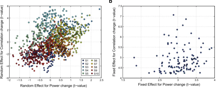
As a control analysis, we checked whether the changes in FC

across areas reflected more than just a change in HGA at the

group level. To do so, we analyzed the relationship between

changes with respect to baseline in HGA and linear correlation

across participants. Given that such across-subjects variability is

modeled by the slope-coefficient in the random terms (i.e., b

(t)

in Eq. 12), we plotted the relationship between the t-values

asso-ciated with b

(t) arising from the linear correlation analysis and

the mean t-values averaged over time (from

⫺1 s to 0.5 s around

movement onset) for the HGA modulations of the

correspond-ing BAs (

Fig. 8

a). Each participant is depicted in a different color,

and each dot is a given a pair of BAs displaying significant

in-crease in linear correlation. The plot shows that participants

dis-playing high changes in power also show high modulations in

Table 2. Statistical results of HGA analysis

ROI number Brodmann area Peak t-value Peak

time (s) Beginning (s) End (s) Duration (s)

1 40 L 14.91 ⫺0.06 ⫺0.32 0.23 0.55 2 1-2-3 L 11.78 ⫺0.06 ⫺0.31 0.26 0.57 3 5 L 11.59 ⫺0.05 ⫺0.36 0.29 0.65 4 6 R 10.66 0.09 ⫺0.43 0.17 0.6 5 29 R 10.37 ⫺0.16 ⫺0.34 ⫺0.03 0.32 6 5 R 10.3 ⫺0.16 ⫺0.34 0.22 0.56 7 31 R 10.03 ⫺0.16 ⫺0.38 0.13 0.51 8 4 L 9.94 ⫺0.04 ⫺0.36 0.26 0.61 9 6 L 9.92 ⫺0.04 ⫺0.4 0.27 0.67 10 4 R 9.52 ⫺0.19 ⫺0.34 0.18 0.51 11 31 L 9.49 ⫺0.16 ⫺0.41 0.29 0.69 12 40 R 9.46 ⫺0.3 ⫺0.36 ⫺0.11 0.25 13 24 R 9.23 ⫺0.2 ⫺0.36 0.2 0.56 14 24 L 8.65 ⫺0.15 ⫺0.36 0.24 0.6 15 7 L 8.62 0.1 ⫺0.44 0.36 0.8 16 39 R 8.61 ⫺0.27 ⫺0.5 ⫺0.11 0.39 17 7 R 8.36 ⫺0.09 ⫺0.44 0.18 0.61 18 30 R 8.29 ⫺0.16 ⫺0.36 ⫺0.04 0.32 19 8 L 8.11 ⫺0.11 ⫺0.26 0.1 0.36 20 1-2-3 R 8.01 0.11 0.02 0.17 0.15 21 29 L 8 ⫺0.16 ⫺0.27 ⫺0.03 0.25 22 32 L 7.84 ⫺0.07 ⫺0.26 0.16 0.41 23 39 L 7.84 ⫺0.07 ⫺0.39 0.17 0.56 24 1-2-3 R 7.73 ⫺0.19 ⫺0.34 ⫺0.11 0.23 25 32 R 7.32 0.09 ⫺0.23 0.15 0.38 26 9 L 7.15 ⫺0.11 ⫺0.23 ⫺0.01 0.22 27 13 L 6.96 ⫺0.11 ⫺0.23 0.21 0.44 28 19 R 6.55 ⫺0.32 ⫺0.43 ⫺0.11 0.32 29 8 R 6.31 ⫺0.2 ⫺0.23 ⫺0.03 0.2 30 41 L 6.21 ⫺0.11 ⫺0.22 ⫺0.06 0.16 31 37 L 6.19 ⫺0.33 ⫺0.35 ⫺0.25 0.1 32 19 R 6.17 0.48 0.42 0.53 0.12 33 43 L 6.14 ⫺0.16 ⫺0.19 ⫺0.04 0.16 34 30 L 6.08 ⫺0.14 ⫺0.38 0.02 0.4 35 43 L 6.04 0.16 0.11 0.21 0.1 36 30 L 5.75 ⫺0.43 ⫺0.53 ⫺0.39 0.15 37 17 R 5.73 ⫺0.22 ⫺0.36 ⫺0.07 0.29 38 18 R 5.7 ⫺0.32 ⫺0.41 ⫺0.06 0.35 39 29 L 5.6 0.1 ⫺0.02 0.11 0.13 40 19 L 5.22 ⫺0.41 ⫺0.44 ⫺0.18 0.26 41 19 L 5.14 ⫺0.13 ⫺0.16 ⫺0.06 0.11

linear correlation, and vice-versa. Indeed, the Pearson’s

correla-tion between changes in HGA and the linear correlacorrela-tion was

highly significant across participants (r

⫽ 0.4495, p ⫽ 9.33e-59).

We then tested whether such relationship was present also at the

group level. To do so, we plotted the same relationship for fixed

effects (

Fig. 8

b). In this case, the Pearson’s correlation between

changes in HGA and FC was r

⫽ 0.1483, and it was not significant

( p

⫽ 0.112). These results therefore suggest that a systematic

−1 −0.5 0 0.5 −2 0 2 4 6 8 10 12 t−value Time (s) −1 −0.5 0 0.5 1 0.01 0.0001 1e−06 1e−08 1e−10 1e−12 1e−14 1e−16 1e−18 1e−20 1e−22 1e−24 1e−26 1e−28 1e−30 1e−32 p−value Time (s) −1 −0.8 −0.6 −0.4 −0.2 0 0.2 0.4 0 10 20 30 40 50 60 70 80 90 100 Significant timepoints (% ) Time (s) BA 7 L BA 1−2−3 L BA 4 L BA 6 L BA 8 L

a

b

c

Figure 6. The time course of activation of t values (a) and associated p values (b) for different sensorimotor and premotor BAs. c, Time course of the percentage of time points showing exemplar sensorimotor and premotor areas.

Figure 7. FC between visuomotor-related BAs. a, Connectivity matrix associated with linear correlation analysis between BAs within the visuomotor-related cortical network. b, Connectivity matrix associated with significant increases in total Granger interdependence between BAs. Graphical representation of linear correlation (c), total Granger interdependence (d), and directed Granger causality graphs (e). Node color is the strength of BAs, defined as the total correlation of each BA with the rest of the network. For Granger causality, the node strengths consider both incoming and outcoming values.

relationship between HGA modulations and FC measures is

pres-ent across participants and needs to be taken into account in the

statistical analyses. Given that we analyzed fixed-effects only, our

results are therefore not contaminated by such confound.

Link communities of visuomotor networks

A critical step in the analysis of networks is the detection of

com-munities, or groups of nodes potentially corresponding to

functional subunits or modules (

Girvan and Newman, 2002

).

Communities, however, may overlap (i.e., a given node may

be-long to more than one group). Large-scale cortical networks may

be no exception. Link communities (i.e., groups of links rather

that nodes) provide an appropriate framework capturing the

re-lationships between overlapping communities while revealing

hi-erarchical organization (

Ahn et al., 2010

). We adopted such

framework for the analysis of adjacency matrices based on linear

correlation and Granger causality networks to identify functional

subnetworks.

Figure 9

a shows the partition density, which

mea-sures the quality of a link partition, as a function of dendrogram

level for both linear correlation and total Granger

interdepen-dence. Link communities were found by cutting the dendrogram

at the maximum partition density D (

Ahn et al., 2010

). The

num-ber of link communities for the linear correlation and total

Granger interdependence was 17 and 5, respectively. For each

link community, we computed its strength, defined as the sum of

node strengths within each link community with respect to the

total node strength of the entire network.

Figure 9

b shows the link

community strength and shows that the first link communities

−2 −1.5 −1 −0.5 0 0.5 1 1.5 2 2.5 −6 −4 −2 0 2 4 6

Random Effect for Power change (t−value)

Random Ef fect for C orrelation change (t −value) S1 S2 S3 S4 S5 S6 S7 S8 S9 S10 1.5 2 2.5 3 3.5 4 4 4.5 5 5.5 6 6.5 7 7.5

Fixed Effect for Power change (t−value)

Fixed Ef

fect for C

orrelation change (t

−value)

a

b

Figure 8. Relationship between changes in HGA and linear correlation. a, Across-subjects variability in HGA and linear correlation accounted by the random-effect term; each participant is depicted in a different color, and each dot is the t-value associated with the random-effect coefficients. b, Fixed-effect t-values for significant pairs of BAs.

Figure 9. Link community analysis. a, Partition density as a function of the link dendrogram cut threshold for linear correlation (black curve) and total Granger interdependence (red). The threshold at which the dendrogram is cut corresponds to the threshold where the maximum partition density was found. b, Community strength for linear correlation (black curve) and total Granger interdependence (red) as a function of link community number. Most representative link community (functional subnetwork) for (c) linear correlation and (d) total Granger interdependence graph.