The dimensionality of stability depends on disturbance type

(1)

RESEARCH OUTPUTS / RÉSULTATS DE RECHERCHE

Author(s) - Auteur(s) :

Publication date - Date de publication :

Permanent link - Permalien :

Rights / License - Licence de droit d’auteur :

Institutional Repository - Research Portal

Dépôt Institutionnel - Portail de la Recherche

researchportal.unamur.be

University of Namur

The dimensionality of stability depends on disturbance type

Radchuk, Viktoriia; DE LAENDER, Frederik; Cabral, Juliano Sarmento; Boulangeat, Isabelle;

Crawford, Michael; Bohn, Friedrich; Raedt, Jonathan De; Scherer, Cédric; Svenning, Jens

Christian; Thonicke, Kirsten; Schurr, Frank M.; Grimm, Volker; Kramer-Schadt, Stephanie

Published in:

Ecology Letters

DOI:

10.1111/ele.13226

Publication date:

2019

Document Version

Peer reviewed version

Link to publication

Citation for pulished version (HARVARD):

Radchuk, V, DE LAENDER, F, Cabral, JS, Boulangeat, I, Crawford, M, Bohn, F, Raedt, JD, Scherer, C,

Svenning, JC, Thonicke, K, Schurr, FM, Grimm, V & Kramer-Schadt, S 2019, 'The dimensionality of stability

depends on disturbance type', Ecology Letters, vol. 22, no. 4, pp. 674-684. https://doi.org/10.1111/ele.13226

General rights

Copyright and moral rights for the publications made accessible in the public portal are retained by the authors and/or other copyright owners and it is a condition of accessing publications that users recognise and abide by the legal requirements associated with these rights. • Users may download and print one copy of any publication from the public portal for the purpose of private study or research. • You may not further distribute the material or use it for any profit-making activity or commercial gain

• You may freely distribute the URL identifying the publication in the public portal ?

Take down policy

If you believe that this document breaches copyright please contact us providing details, and we will remove access to the work immediately and investigate your claim.

(2)

The dimensionality of stability depends on disturbance type

1 2

Running title: dimensionality of ecological stability 3

Viktoriia Radchuk1_{, Frederik De Laender}2_,_{Juliano Sarmento Cabral}3_{, Isabelle Boulangeat}4,5_,

4

Michael Crawford6_{, Friedrich Bohn}7_{, Jonathan De Raedt}2,8_{, Cédric Scherer}1_{, Jens-Christian}

5

Svenning4,9_{, Kirsten Thonicke}10_{, Frank Schurr}11_{, Volker Grimm}7,6,12_{, Stephanie}

Kramer-6

Schadt1,13

7 8

1 _{Department of Ecological Dynamics, Leibniz Institute for Zoo and Wildlife Research (IZW),}

Alfred-9

Kowalke-Straße 17, Berlin, Germany, radchuk@izw-berlin.de, scherer@izw-berlin.de

10

2_{Institute of Life-Earth-Environment, Namur Institute of Complex Systems, Research Unit in}

11

Environmental and Evolutionary Biology. Université de Namur, Rue de Bruxelles 61, Namur, Belgium,

12

frederik.delaender@unamur.be

13

3 _{Ecosystem Modeling,} _{Center for Computational and Theoretical Biology (CCTB), University of}

14

Würzburg, Campus Hubland Nord, Würzburg, Germany, juliano.sarmento_cabral@uni-wuerzburg.de

15

4 _{Section for Ecoinformatics and Biodiversity, Department of Bioscience, Aarhus University, Ny}

16

Munkegade 116, Aarhus, Denmark, isabelle.boulangeat@gmail.com

17

5_{Univ. Grenoble Alpes, Irstea, UR LESSEM, 2 rue de la Papeterie-BP 76, F-38402 St-Martin-d'Hères,}

18

France

19

6 _{Institute for Biochemistry and Biology, University of Potsdam, Maulbeerallee 2, Potsdam, Germany,}

20

mscrawfor@gmail.com

21

7_{Department of Ecological Modelling, Helmholtz Centre for Environmental Research – UFZ,}

22

Permoserstr. 15, Leipzig, Germany, friedrich.bohn@ufz.de

23

8_{Laboratory of Environmental Toxicology and Aquatic Ecology, Ghent University, Coupure Links 653,}

24

Ghent, Belgium, jonathan.deraedt@ugent.be

25

9 _{Center for Biodiversity Dynamics in a Changing World (BIOCHANGE), Aarhus University, Ny}

26

Munkegade 114, Aarhus, Denmark, svenning@bios.au.dk

27

10_{Research Domain 1 “Earth System Analysis”, Potsdam Institute for Climate Impact Research (PIK),}

28

Telegrafenberg A31, Potsdam, Germany, kirsten.thonicke@pik-potsdam.de

29

11_{Institute of Landscape and Plant Ecology, University of Hohenheim, August-von-Hartmann-Str. 3,}

30

Stuttgart, Germany, frank.schurr@uni-hohenheim.de

31

Mis en forme : Anglais (États-Unis) Mis en forme : Anglais (États-Unis) Mis en forme : Anglais (États-Unis) Mis en forme : Anglais (États-Unis) Mis en forme : Français (Belgique) Mis en forme : Anglais (États-Unis) Mis en forme : Anglais (États-Unis) Mis en forme : Anglais (États-Unis) Mis en forme : Anglais (États-Unis) Mis en forme : Anglais (États-Unis)

Mis en forme : Anglais (États-Unis) Mis en forme : Anglais (États-Unis) Mis en forme : Anglais (États-Unis) Mis en forme : Anglais (États-Unis) Mis en forme : Anglais (États-Unis) Mis en forme : Anglais (États-Unis) Mis en forme : Anglais (États-Unis) Mis en forme : Anglais (États-Unis) Mis en forme : Anglais (États-Unis) Mis en forme : Anglais (États-Unis) Mis en forme : Anglais (États-Unis)

(3)

12 _{German Centre for Integrative Biodiversity Research (iDiv) Halle-Jena-Leipzig, Deutscher Platz 5e,}

32

Leipzig, Germany, volker.grimm@ufz.de

33

13_{Department of Ecology, Technische Universität Berlin, Rothenburgstrasse 12, 12165 Berlin,}

34

kramer@izw-berlin.de 35

36

Corresponding author: radchuk@izw-berlin.de

37 38

This manuscript type is a Letter 39

Word count in abstract: 150 40

Word count main text: 4951 41

Word count in Glossary: 310 42 Number of references: 55 43 Number of figures: 5 44 Number of tables: 0 45

Statement of authorship: All authors discussed and agreed on the experimental design; 46

MC, FB, JDR, CS and VR run the simulations; VR performed the analyses of stability; VR wrote 47

the first draft of the manuscript and all authors contributed substantially to revisions. 48

Data accessibility statement: should the manuscript be accepted, the data supporting the 49

results will be archived in an appropriate public repository (Dryad or Figshare) and the data DOI 50

will be included at the end of the article. 51

Mis en forme : Anglais (États-Unis) Mis en forme : Anglais (États-Unis) Mis en forme : Anglais (États-Unis) Mis en forme : Anglais (États-Unis) Code de champ modifié

(4)

ABSTRACT

52

Ecosystems respond in various ways to disturbances. Quantifying ecological stability therefore 53

requires inspecting multiple stability properties, such as resistance, recovery, persistence, and 54

invariability. Correlations among these properties can reduce the dimensionality of stability, 55

simplifying the study of environmental effects on ecosystems. A key question is how the kind of 56

disturbance affects these correlations. We here investigated the effect of three disturbance types 57

(random, species-specific, local) applied at four intensity levels, on the dimensionality of 58

stability at the population and community level. We used previously parameterized models that 59

represent five natural communities, varying in species richness and the number of trophic levels. 60

We found that disturbance type but not intensity affected the dimensionality of stability and only 61

at the population level. The dimensionality of stability also varied greatly among species and 62

communities. Therefore, studying stability cannot be simplified to using a single metric and 63

multi-dimensional assessments are still to be recommended. 64

65 66

Keywords: Community model, persistence, resistance, invariability, recovery, extinction, 67

disturbance intensity, disturbance type, individual-based model 68

Mis en forme : Anglais (États-Unis)

(5)

GLOSSARY

69

State variables are variables used to quantify stability properties of a system, i.e. a 70

population or a community in the context of this study. Examples of state variables are 71

abundance (population level) and species richness or total abundance (community level). 72

Resistance is the degree to which a state variable is changed following a disturbance 73

(Pimm 1984), here measured as the difference between a perturbed and a control system at the 74

first sampling after the treatment (Hillebrand et al. 2018). 75

Recovery is the capacity of a system to return to its undisturbed state following a 76

disturbance (Ingrisch & Bahn 2018), here measured as the degree of change in a state variable of 77

a perturbed compared to a control system at the last sampling (Hillebrand et al. 2018). 78

Persistence is the existence of a system through time as an identifiable unit (Pimm 1984; 79

Grimm & Wissel 1997), measured by the time during which a system maintains the same state 80

(i.e., state variables within certain ranges) before it changes in some defined way (Donohue et al. 81

2016). 82

Invariability reflects the temporal constancy of a state variable following the 83

disturbance, usually measured as the inverse of temporal variability of a state variable (Wang et 84

al. 2017). Higher invariability indicates higher stability (Donohue et al. 2013).

85

Disturbance is a change in the biotic or abiotic environment that alters the structure and 86

dynamics of a system (Donohue et al. 2016). 87

Stability is a multidimensional concept that tries to capture the different aspects of the 88

dynamics of the system and its response to perturbations (Donohue et al. 2016). Here, we 89

consider the following stability properties: resistance, recovery, persistence, and variability. 90

Mis en forme : Anglais (États-Unis) Mis en forme : Anglais (États-Unis) Mis en forme : Anglais (États-Unis) Mis en forme : Anglais (États-Unis)

Mis en forme : Anglais (États-Unis) Mis en forme : Anglais (États-Unis) Mis en forme : Anglais (États-Unis) Mis en forme : Anglais (États-Unis) Mis en forme : Anglais (États-Unis) Mis en forme : Anglais (États-Unis) Mis en forme : Anglais (États-Unis) Mis en forme : Anglais (États-Unis)

Mis en forme : Anglais (États-Unis) Mis en forme : Anglais (États-Unis)

(6)

The dimensionality of stability (DS) depends on the strength of correlations among 91

stability properties. Low correlation corresponds to high dimensionality. If dimensionality is 92

high, a single stability measure cannot be used as a sole indicator of the overall system stability 93

(Donohue et al. 2013).

94 Mis en forme : Anglais (États-Unis)

(7)

INTRODUCTION

95

Understanding the response of populations, communities, and ecosystems to fast, human-induced 96

environmental changes is a key challenge (Carpenter et al. 2011; Higgins & Scheiter 2012; 97

Scheffer et al. 2015; DeLaender et al. 2016). However, quantifying the stability of natural 98

systems is challenging because stability is a multidimensional concept and requires measuring 99

several stability properties such as resistance, recovery, persistence, and invariability (see 100

Glossary, Pimm 1984; Grimm & Wissel 1997; Donohue et al. 2016). Correlation among these 101

properties manifests the dimensionality of stability (DS): if the stability properties strongly 102

correlate, the dimensionality is low, and vice versa (Donohue et al. 2013; Hillebrand et al. 2018, 103

Fig. 1a,b). Theory underpinning DS is still in its infancy (Donohue et al. 2013) and relevant 104

empirical evidence is only beginning to accumulate (Donohue et al. 2013; Hillebrand et al. 105

2018). A key question is whether DS depends on the kind of underlying disturbance. Donohue et 106

al. (2013) showed that when disturbed by consumer removal, DS increased in marine shore

107

communities. At present it is unclear if such conclusions can be extrapolated to other kinds of 108

disturbance. 109

There are many kinds of disturbance. Disturbance properties include: duration, spatial 110

extent, intensity, frequency, and type (Turner 2010). According to their duration, two extreme 111

classes of disturbance can be distinguished: pulse disturbances (e.g. fire or flooding) occur over a 112

short time scale, relative to the typical speed at which a system changes, and press disturbances 113

(e.g. global warming or exploitation) represent a constant, long-term change. Disturbance 114

intensity reflects how much individuals / biomass are affected by an event over a period of time

115

(Turner 2010). Disturbance frequency reflects how often disturbance events occur within a given 116

Commenté [FDL1]: There’s a space missing: ‘De Laender’, not

‘DeLaender’

Mis en forme : Anglais (États-Unis) Mis en forme : Anglais (États-Unis) Mis en forme : Anglais (États-Unis) Mis en forme : Anglais (États-Unis) Mis en forme : Anglais (États-Unis) Mis en forme : Anglais (États-Unis) Mis en forme : Anglais (États-Unis) Mis en forme : Anglais (États-Unis)

(8)

time period. Examples of disturbance types are local vs. global, and selective vs. non-selective 117

disturbances (De Laender et al. 2016). 118

Despite increasing understanding of how disturbances affect each single stability 119

property, we know little of how the kind of disturbance affects the relationships among multiple 120

stability properties, i.e. the dimensionality of stability (Donohue et al. 2013). Yet, such 121

knowledge is crucial for guiding efforts to monitor and manage natural systems. Indeed, if 122

several stability properties correlate strongly irrespective of the properties of disturbances acting 123

on them, the stability of the overall system reduces to one dimension (i.e. low DS, Fig. 1a). This 124

means that monitoring schemes could be optimized by quantifying only a few stability 125

properties. Vice versaAlternatively, if a system's stability properties are poorly correlated (i.e. 126

high dimensionality), inferring the system's overall stability requires measuring all of 127

themproperties (Fig. 1b). Therefore, management of natural systems would profit from knowing 128

how DS is influenced by different disturbance properties. For example, an increase of 129

dimensionality with disturbance intensity would undermine the main assumption for detecting 130

tipping points (Dakos et al. 2012; Dai et al. 2015) through early warning signals (e.g. coefficient 131

of variation, temporal autocorrelation), which usually manifest the variability of a system. 132

DS can be decomposed into pair-wise correlations among underlying stability properties 133

(Donohue et al. 2013; Hillebrand et al. 2018; Pennekamp et al. 2018). We generally expect 134

positive pair-wise correlations between invariability, resistance, recovery and persistence. For 135

example, at the population level invariability and persistence are expected to correlate positively 136

at the population level, because the higher the temporal constancy in population size, the more 137

likely the population is to persist (Ginzburg et al. 1982; Inchausti & Halley 2003). Similarly, at 138

Mis en forme : Anglais (États-Unis) Mis en forme : Anglais (États-Unis) Mis en forme : Anglais (États-Unis)

(9)

likely this community is to persist in its unchanged state. For arguments of why we expect other 140

stability properties to correlate positively, see Table S1 in Supporting Information. Because pair-141

wise correlations are ‘constituents’ of DS, they are expected to depend on the same factors as 142

DS: disturbance properties and the level of organization. Indeed, the sign of a pair-wise 143

correlation between stability properties was shown to change when, instead of a single 144

disturbance, two disturbance types were applied simultaneously to yeast populations (Dai et al. 145

2015). Also, pair-wise correlations measured at the community and ecosystem level differed in 146

plankton communities disturbed by reduced light availability (Hillebrand et al. 2018). 147

Understanding whether pair-wise correlations are affected similarly by across disturbances 148

irrespective ofdifferent disturbance types and study systems would facilitate more efficient 149

monitoring of the stability of natural systems. 150

Here, we used process-based, spatially-explicit models to assess how the intensity and the 151

type of disturbance affect DS at the population and community levels. Our models are well tested 152

and structurally realistic, and represent five different communities: a species-rich temperate 153

grassland community, a temperate forest, an algae community, a boreal predator-prey system, 154

and a host-pathogen system. The modelled communities varied in species richness (2 up to 86 155

species) and number of trophic levels (one or two). At both levels of organization we measured 156

four stability properties: resistance, recovery, persistence, and invariability (Glossary, Fig. 2a-c, 157

Table S2). We applied three disturbance types at four intensities. We distinguished disturbances 158

that i) affect individuals selectively depending on their species identity, ii) affect individuals 159

selectively depending on their location, and iii) affect all individuals similarly, irrespective of 160

species identity or location (Fig. 2d,e,f). We tested the following hypotheses: 161

H1: At each level of organization, DS depends on disturbance type and intensity. 162

(10)

H2: All investigated stability properties exhibit positive pairwise correlations (Table S1). 163

H3: At each level of organization, the pair-wise correlations depend on disturbance type 164

and intensity. 165

(11)

METHODS

166

Study systems 167

We used models representing the dynamics of the following communities: temperate 168

forests (Bohn et al. 2014), a marine algal community (Baert et al. 2016a), a species-rich 169

temperate grassland (May et al. 2009), a boreal predator-prey system of mustelids and voles 170

(Radchuk et al. 2016a), and a temperate host-pathogen system of classical swine fever (CSF) 171

virus affecting wild boar populations (Kramer-Schadt et al. 2009; Lange et al. 2012). All of these 172

models had previously been parameterized to mimic the conditions of the respective natural 173

communities (Table S3). All models have three aspects in common: 1) they are spatially explicit, 174

describing the location of habitat patches and movement of individuals among them; 2) they 175

include demographic stochasticity; and 3) the smallest modelled entity is the individual (except 176

for the model simulating an algae community, which is based on Lotka-Volterra equations with a 177

dispersal component; Supplementary Text T1). In addition to demographic stochasticity, two 178

models (a host-pathogen model and a model of temperate forests) also include environmental 179

stochasticity. Temperate grassland was modelled in two ways: using the original IBC-grass 180

model (May et al. 2009) and a modified version that incorporates intra-specific trait variation 181

(from now on referred to as Grassland ITV, Crawford et al. 2018). We thus used six models that 182

represented five study systems. An advantage of using models that have been previously 183

developed is bcause that those models have already been tested and verified for respective 184

natural systems. We provide short summaries of the main processes included in each model in 185

the Supplementary Methods, and more detailed descriptions of the models in the Supplementary 186

Texts T1-T5. 187

Mis en forme : Anglais (États-Unis) Mis en forme : Anglais (États-Unis) Mis en forme : Anglais (États-Unis) Mis en forme : Anglais (États-Unis) Mis en forme : Anglais (États-Unis) Mis en forme : Anglais (États-Unis) Mis en forme : Anglais (États-Unis) Mis en forme : Anglais (États-Unis) Mis en forme : Anglais (États-Unis) Mis en forme : Anglais (États-Unis) Mis en forme : Anglais (États-Unis) Mis en forme : Anglais (États-Unis) Mis en forme : Anglais (États-Unis)

(12)

188

Disturbances 189

The previously published versions of the models, parameterized to reflect a stochastic 190

quasi-equilibrium state (Nolting & Abbott 2016), were used as a control (no disturbance). We 191

implemented disturbance as a one-time (pulse) removal of individuals. We implemented three 192

types of disturbance (Fig. 2d, e, f): random disturbance affected individuals randomly, 193

irrespective of their species identity and location. This disturbance type reflects a non-selective 194

disturbance (De Laender et al. 2016). The rare species removal disturbance reflects the 195

assumption that the rarest species are most extinction-prone (Solan et al. 2004) and is applied to 196

species inversely to their population abundance ranks. This disturbance type was not possible in 197

the wild boar - virus model (Supplementary Methods). The spatially-structured disturbance 198

mimicked a localized disturbance by randomly selecting a point for the centre of the disturbance 199

and then gradually increasing the disturbance radius around this point until the disturbance 200

affected the target number of individuals (as defined by the disturbance intensity). We have 201

implemented disturbance types via removal of individuals because this is a generic process that 202

is inherent to several real-world disturbances, such as habitat fragmentation, hunting, culling and 203

pollution. Using removal of individuals allows for comparability of results among the models as 204

they differ in their processes. Therefore, removal of individuals was the best compromise among 205

the relevance of the disturbance type and comparability of results among the systems. 206

Each disturbance type was implemented at four intensities, reflecting increasing 207

proportions of the community that were removed (0.1, 0.2, 0.3 and 0.4 respectively). An upper 208

bound of intensity was chosen via preliminary tests scanning a larger range of intensities, which 209

(13)

showed that at a disturbance intensity > 0.5, all species in our 2-species systems went extinct, 210

complicating the measurements of all stability properties. 211

We ensured the comparability of the results in terms of the temporal scales among our 212

study systems by scaling the duration of the simulation runs to the average generation length of 213

all the species in the community (Pimm 1984). We used 30 average generations of the control as 214

a ‘burn-in’ phase, after which either the control or one of the disturbance type scenarios were run 215

for the next 60 generations, which was enough for majority of the species to attain either 216

previous or a new stochastic quasi-equilibrium state (based on Gelman-Rubin diagnostics, 217

Supplementary Figs. S1-S3, Supplementary Methods). The disturbance was applied in the first 218

time step immediately after the ‘burn-in’ phase. We ran 30 replicates of each of the 13 scenarios 219

(the control plus three disturbance types crossed with four levels of disturbance intensity) to 220

account for the stochasticity inherent in the models. These 30 replicates were sufficient to 221

capture effects that are due to disturbances and not merely a result of stochasticity 222

(Supplementary Methods and Figs. S4-S7). The ‘burn-in’ phase was discarded when calculating 223

the stability properties. 224

Stability properties 225

At both the community and population level, we quantified four stability properties: 226

resistance, recovery, persistence and invariability (Glossary, Fig. 2a-c, Table S2). We quantified

227

stability properties analogously at both levels of organization. At the community level as state 228

variable we used community composition, and at the population level we used abundance. We 229

here detail how stability properties were measured at the community level, for details on how it 230

was done at the population level please refer to Supplementary Methods. 231

(14)

Resistance was measured as Bray-Curtis similarity of the community composition

232

between treatment and control at the first sampling after treatment (time step 1, Hillebrand et al. 233

2018). Resistance ranges between 0 and 1 with 1 reflecting maximum resistance (100% 234

similarity between treatment and control). Recovery reflects the degree of restoration of the 235

system at the end of the time series and was measured as Bray-Curtis similarity of the 236

community composition between treatment and control at the final sampling (time step 60, 237

Hillebrand et al. 2018). Analogously to resistance, recovery ranges between 0 and 1, with 1 238

reflecting a full recovery. Persistence was measured as the time during which the community 239

composition in a treatment remains within 90% of the Bray-Curtis similarity with the 240

composition of the control community. We scaled the original persistence values (min = 1, max 241

= 60) by dividing them by their theoretically possible maximum (60), so that persistence ranges 242

from 0 (the similarity between the treatment and control is < 0.9 in the first time step) to 1 243

(maximum persistence, a system remains within 90% of similarity during the whole period). 244

Temporal invariability (Wang et al. 2017) was measured as the inverse of standard deviation of 245

residuals from the linear model regressing the Bray-Curtis similarity between the treatment and 246

control communities on time (Hillebrand et al. 2018). When temporal invariability is higher, i.e. 247

when community composition fluctuates less around the average trend, the stability is higher. In 248

Supplementary Methods we explain the choice of 1) Bray-Curtis similarity as a particularly 249

suitable state variable for measuring stability at the community level (Donohue et al. 2013; 250

Hillebrand et al. 2018) and 2) the threshold of 90% of Bray-Curtis similarity to measure 251

persistence. 252

(15)

Dimensionality of stability 253

We quantified DS using multidimensional ellipsoids based on the covariance matrices 254

among all stability properties (Donohue et al. 2013). The covariance matrices were constructed 255

using the 30 replicates per scenario (at the community level) and per species nested within each 256

scenario (at the population level). Since disturbances may affect both the volume and the shape 257

of such ellipsoids (Donohue et al. 2013, Fig. 1a-c), we considered both. We used semi-axis 258

lengths to characterize the shape of ellipsoids. The semi-axis length 𝑎𝑖 was measured as 𝑎𝑖=

259

𝜆𝑖0.5, where 𝜆𝑖 is the ith eigenvalue of the covariance matrix for a given scenario (i.e. a

260

combination of the disturbance type and intensity) at the community level and for each species 261

within each scenario at the population level. Ellipsoid volume was calculated as 𝑉 = 262

𝜋𝑛⁄2

Γ(𝑛

2+1)

∏𝑛 (𝜆0.5₎

𝑖=1 , where n is the dimensionality of the covariance matrix. Prior to the calculation

263

of the ellipsoid volume, each set of semi-axis lengths was standardized by dividing all of them 264

by the maximum length within a set, so that the maximum standardized length equalled 1. This 265

allowed us to calculate the largest volume that was theoretically possible (i.e. all of the 266

standardized semi-axis lengths are 1), which reflects a perfect spheroidal shape and, therefore, 267

high DS. By dividing the actual ellipsoid volume by the theoretical maximum, we obtained a 268

proportional volume. This proportional volume varies between 0 (a ‘cigar’-like shape of 269

ellipsoids, Fig. 1a), and 1 (a perfect sphere, Fig. 1b), reflecting low and high DS, respectively. 270

Characterization of multidimensional ellipsoids based on covariance matrices relies on the 271

assumption of linear relationships among stability properties (Supplementary Methods). In our 272

case this assumption is satisfied for most study systems and disturbance types (e.g. Figs. S8-273

S15). 274

Mis en forme : Anglais (États-Unis) Mis en forme : Anglais (États-Unis) Mis en forme : Anglais (États-Unis) Mis en forme : Anglais (États-Unis) Mis en forme : Anglais (États-Unis) Mis en forme : Anglais (États-Unis) Mis en forme : Anglais (États-Unis) Mis en forme : Anglais (États-Unis) Mis en forme : Anglais (États-Unis) Mis en forme : Anglais (États-Unis) Mis en forme : Anglais (États-Unis) Mis en forme : Anglais (États-Unis) Mis en forme : Anglais (États-Unis) Mis en forme : Anglais (États-Unis) Mis en forme : Anglais (États-Unis) Mis en forme : Anglais (États-Unis) Mis en forme : Anglais (États-Unis) Mis en forme : Anglais (États-Unis) Mis en forme : Anglais (États-Unis) Mis en forme : Anglais (États-Unis) Mis en forme : Anglais (États-Unis) Mis en forme : Anglais (États-Unis) Mis en forme : Anglais (États-Unis) Mis en forme : Anglais (États-Unis) Mis en forme : Anglais (États-Unis) Mis en forme : Anglais (États-Unis) Mis en forme : Anglais (États-Unis) Mis en forme : Anglais (États-Unis) Mis en forme : Anglais (États-Unis)

(16)

To test the effect of disturbance properties on DS (H1) we fitted generalized mixed-275

effects models (Gamma distribution) with either ellipsoid volume or semi-axis length (per each 276

rank, Fig. 1c) as a response (Supplementary Methods). As fixed effect predictors we included 277

disturbance type (as a factor) and intensity (as a continuous variable). At the community level, 278

we included study system as a random slope and at the population level, the random slope 279

structure consisted of the species nested within the study system. We tested for the significance 280

of fixed-effect terms using likelihood-ratio tests (LRT), but in our interpretations focused on 281

effect sizes, because our study is based on simulations and virtually anything can become 282

significant given enough replicates. At the community level, there was no variation in 283

persistence for at least one disturbance type in the three study systems (persistence was 0 in all 284

replicates of a rare species removal disturbance in both grassland systems and it was 1 in all 285

replicates of random disturbance and rare species removal of the algae system). This precluded 286

calculation of semi-axis lengths and ellipsoid volumes using all four stability properties (i.e. four 287

dimensions) for these study systems. Therefore, we first fitted models using all four dimensions 288

with only three study systems (forest, vole-mustelid, and wild boar-virus), and then used three 289

dimensions (excluding persistence) to fit models with all six study systems. The results from 290

both analyses are qualitatively the same. The results based on three dimensions are presented in 291

the main text, and those based on four dimensions in Fig. S16, Tables S4 and S5. 292

Pair-wise correlations 293

To test whether all pair-wise correlations among stability properties were positive (H2) 294

and affected by the disturbance properties (H3), we calculated Spearman-rank correlation for 295

each pair of stability properties obtained for each of the 13 scenarios at the community level. 296

(17)

within each scenario. Next, we transformed these Spearman-rank correlations into Fisher’s z 298

scores to improve their normality and to avoid any disproportionate influence of extreme values, 299

and used them as effect sizes in the meta-analysis (Koricheva et al. 2013). We fitted mixed-300

effects meta-analytic models (Gaussian distribution) with the fixed effects of disturbance type (a 301

factor), disturbance intensity (a continuous variable), and an interaction between them. At the 302

community level, the models included the study system and replicate as random intercepts. At 303

the population level, also species identity was included as a random intercept. All meta-analytic 304

mixed-effects models were fitted with the library metafor in R (Viechtbauer 2010). All analyses 305

were conducted in R 3.4.2 (R 2017). 306

307

(18)

RESULTS

308

Effect of disturbance properties on the dimensionality of stability 309

At the community level, neither disturbance type nor intensity affected DS (as measured 310

by semi-axis lengths, Fig. 3a & Fig. S17a; and ellipsoid volumes, Fig. 4a & Fig. S18a; Table S4). 311

However, study systems varied in their DS, as measured by semi-axis lengths (Table S6, Fig. 3a) 312

or ellipsoid volumes (Fig. 4a). While grassland and forest communities were characterized by 313

high DS (Fig. 4a), corresponding to spheroid-looking stability ellipsoids (Fig. S19a,b), vole-314

mustelid and algae communities had low DS, corresponding to a ‘cigar’-like ellipsoids. 315

At the population level, the disturbance intensity did not affect DS (Fig. S18b), while 316

disturbance type did (Table S4). Random disturbance increased DS (Fig. 4b). This was also 317

reflected in the differences among semi-axis lengths: under random disturbance, the semi-axis 318

lengths of the 1st_{rank were shorter}_{compared tothan for}_{other disturbance types, and the}

semi-319

axis lengths of the 3rd and 4th order were longer than for compared to other disturbance types 320

(Fig. 3b). At the population level, DS varied among study systems and species (Fig. 4b, Table 321

S5). 322

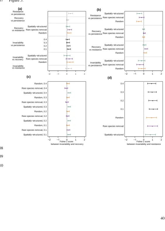
Pair-wise correlations between stability properties 323

At the community level, pair-wise correlations were on average positive (supporting H2) 324

and three out of six correlations were affected by disturbance properties (supporting H3, Fig. 5a). 325

The Correlation correlation of recovery with resistance and of recovery with invariability 326

depended on the disturbance type, with positive correlations under random disturbance and very 327

weak correlations (around 0) under spatially-structured disturbance. The Correlation correlations 328

Mis en forme : Anglais (États-Unis) Mis en forme : Anglais (États-Unis) Mis en forme : Anglais (États-Unis) Mis en forme : Anglais (États-Unis) Mis en forme : Anglais (États-Unis) Mis en forme : Anglais (États-Unis)

(19)

between invariability and persistence became weaker and approached 0 as disturbance intensity 329

increased. 330

At the population level, two pair-wise correlations were on average negative, three were 331

positive, and one correlation was close to 0 (Fig. 5b-d). All pair-wise correlations were affected 332

to a certain degree by disturbance type (Table S7). Additionally, disturbance intensity interacted 333

with disturbance type in its effect on one correlation (invariability with recovery, Fig. 5c) and 334

affected another one (invariability with resistance) in an additive way (Fig. 5d). There was no 335

coherent pattern in how disturbance type modulated different pair-wise correlations. 336

(20)

DISCUSSION

337

We tested whether the correlation structure among stability properties was affected by the 338

disturbance properties across five communities, differing in species richness and number of 339

trophic levels. Contrary to our expectation (H1), At the community level, we did not find an 340

effect of the disturbance properties on the dimensionality of stability (DS) at the community 341

level(DS, H1). At the population level, DS was higher under random disturbances. Additionally, 342

at both levels of organization DS varied largely among study systems. At the community level, 343

as expected (H2), we found generally positive correlations among different stability properties. 344

In contrast, at the population level, the sign and magnitude of correlations were highly 345

heterogeneous. Finally, pair-wise correlations at both levels depended on the disturbance 346

properties, mainly on disturbance type, supporting our hypothesis (H3), although the effect sizes 347

were smaller at the community level. 348

Dimensionality of stability at the community and population level 349

We did not find any effect of disturbance properties on DS at the community level. 350

However, our findings reveal high heterogeneity in DS among study systems. For 4 of the 6 351

study systems, community stability was a highly-dimensional concept (Fig. 4a), suggesting that 352

monitoring these systems requires measuring multiple stability properties. A promising avenue 353

for future research would be investigating whether – and what – properties of a system predict its 354

DS. At the community level, our findings indicate that such candidates of system properties as 355

species richness and number of trophic levels do not discriminate the systems with low and high 356

DS (Fig. S20a,b). Indeed, our two species-poor systems (‘vole-mustelid’ and ‘wild boar-virus’) 357

exhibited strikingly different DS (Fig. 4a). Similarly, we observed both high and low DS in 358

(21)

vs ‘wild boar-virus’). Taken together our results indicate that, although DS does not depend on 360

disturbance properties, measuring multiple stability properties is necessary until we can establish 361

whether and what system properties underlie DS. 362

Similarly to the community level, DS was highly context-dependent at the population 363

level: in addition to variation among disturbance types, we also found high heterogeneity among 364

study systems and species (Table S5), with the highest dimensionality under random disturbance. 365

Although this type of disturbance may seem of little relevance to real-world applications, it is 366

closely mimicked by the application of certain chemicals (Roessink et al. 2006; DeLaender et al. 367

2016), and therefore its effects on DS deserve further investigations. Interestingly, our findings 368

indicate that species-poor systems may generally have higher DS (Fig. S20d). Since population 369

invariability is known to be lower in species-rich systems (Gonzalez & Descamps-Julien 2004; 370

Jiang & Pu 2009; Gross et al. 2014), it is likely that species richness modulates the relations of 371

population-level invariability with other stability properties. However, as we did not 372

experimentally manipulate species richness in this study, this is a hypothesis to be tested by 373

future research. 374

Reflecting the context-dependence of DS, all pair-wise correlations between population 375

stability properties depended on the disturbance type, and additionally two out of six depended 376

on the disturbance intensity (Fig. 5b-d). These results corroborate earlier analytical derivations 377

(Harrison 1979) that showed that the relation between population resilience and resistance 378

depends both on density-dependence and on the environmental sensitivity of the population 379

growth rate. In fact, the high heterogeneity found in the meta-analytic models testing the context-380

dependence of the pair-wise correlations between population stability properties (Table S8) 381

points towards species-specific differences which may be due to differences in density 382

Code de champ modifié

(22)

dependence (as found by Harrison 1979) or any other species-specific properties (e.g. population 383

growth, carrying capacity). 384

From a monitoring perspective, the context-dependence of the correlative structure 385

among stability properties at the population level (H3) means that quantification of population 386

stability as a whole requires measurements of multiple stability properties unless the context-387

dependence of these properties was established beforehand. Even though this may sound like a 388

daunting task, it is already a well-established practice within population viability analysis 389

(Beissinger & Westphal 1998; Pe’er et al. 2013). In such studies, multiple stability properties 390

such as time to extinction, minimum viable population size, mean population size, etc. are jointly 391

reported as a rule (Pe’er et al. 2013). 392

Across-system differences in dimensionality of stability and plausible 393

mechanisms 394

We did not find any effect of disturbance type on DS at the community level but higher 395

DS was observed for random disturbances at the population level. Although these general results 396

hold across the five different study systems, the largest heterogeneity in DS was revealed among 397

study systems. As mentioned above, this heterogeneity cannot be explained by system properties 398

as species richness and number of trophic levels. Two general mechanisms behind the responses 399

of system’s DS to disturbance can be distinguished: changes in the intensity of species 400

interactions and changes in the degree of stochastic dynamics of the system. Although we have 401

not experimentally manipulated these mechanisms here, we discuss the revealed differences in 402

DS among systems in light of these mechanisms. 403

(23)

Changes in the intensity of species interactions could explain the link between 404

disturbances and DS. Indeed, previous research demonstrated that inter- and intra-specific 405

interactions affect community stability (McCann 2000; Thébault & Loreau 2005; Barabás et al. 406

2016). Moreover, the effect of changes in species interactions on DS may differ depending on 407

the primary type of interactions within a system (competitive vs. trophic), because vertical 408

diversity was shown to modulate the biodiversity – stability relationship (Reiss et al. 2009; 409

Radchuk et al. 2016b)+Wang and Brose’s Ecology Letters from last year (‘vertical diversity 410

hypothesis’). Indeed, in our simulations, the removal of a rare species removal in from 411

communities driven by competitive interactions (algae, grassland and forest systems) resulted in 412

lower DS (Table S9) both at the community and population level. The mechanism underlying the 413

lower DS in these communities after removal of rare species (Table S9) may be an increasing 414

strength of competitive interactions among the remaining species. 415

Stronger competitive interactions presumably occurring after removal of rare species, 416

may in turn lead to more deterministic dynamics of the system. The degree of dynamic system 417

behaviour may itself affect DS. Indeed, a more stochastic population dynamics likely results in 418

weaker pair-wise correlation among stability properties, thus leading to higher DS. In support of 419

this expectation, we found increased DS after a spatially-structured disturbance in systems 420

consisting of two strongly interacting species at different trophic levels (Table S9). Such two-421

species communities are presumably more prone to stochastic effects than multispecies 422

communities, and therefore exhibit the above-described behaviour. To closer inspect the relation 423

between system stochastic behaviour and DS, we used population abundance and community 424

evenness the followingas proxies of the influence of demographic stochasticity at the on 425

populations and community communitieslevel, respectively: population abundance and 426

(24)

community evenness (Supplementary Methods). Overall, we found an increase in DS under 427

higher stochasticity at both population and community levels (Fig. S21-S22). However, the 428

responses varied among disturbance types, study systems and species (for the population-level 429

DS; Figs S23-S24). Importantly, these findings have to be treated with caution because Clearly, 430

we did not experimentally vary stochasticity, as this was not the goal of our study. , and Future 431

future research in this direction is warranted. 432

The change of system behaviour from stochastic to deterministic and vice versa may also 433

be caused by dispersal. Dispersal plays an important role in stochastic community assembly 434

(Chase 2007) and has recently attracted attention in the context of metapopulation and 435

metacommunity stability (Dai et al. 2013; De Raedt et al. 2017; Gilarranz et al. 2017; Zelnik et 436

al. 2018). Further, functional diversity, in particular response diversity and correlations among

437

effect and response traits were suggested as mechanisms potentially explaining pair-wise 438

correlations between stability properties (Pennekamp et al. 2018). Additionally, some of the 439

observed differences in system responses may be due to the model type used and not especially 440

because of the system-specific characteristics. Thus, models such as the Lotka-Volterra model 441

(used for the algae community) result in more deterministic community dynamics compared to 442

individual-based models that incorporate more stochasticity at different levels and processes. 443

Indeed, the algae model showed a strikingly clear response as compared to other systems (Table 444

S9, Fig. 4a), which may be explained by deterministic system behavior. 445

Challenges and future research 446

Our study identified several challenges associated with measuring DS, . for example Amongst 447

those are: quantifying the relationships among stability properties that are non-linearly related;, 448

(25)

properties at each level of organization;, deciding on the disturbance types and intensity levels. A 450

wide variety of stability properties is used in the literature, and different approaches to 451

quantifying them are available (Grimm & Wissel 1997; Ingrisch & Bahn 2018). For example, we 452

have chosen to measure resistance at the first time step after disturbance. An alternative would be 453

to measure resistance at the time step when the response is the strongest, which, naturally, will 454

differ among species and systems. Comparison of how existing stability properties and methods 455

to measure them perform under different conditions and unification of such approaches must beis 456

an avenue for future research (Ingrisch & Bahn 2018). Further, we here focused on disturbance 457

by removing individuals mainly for the sake of comparability of results among systems and 458

models. What the implications of other disturbance types are, in particular the addition of 459

individuals (stocking) and habitat fragmentation are, and how they compare to the removal of 460

individuals, remains to be tested. 461

Further, a future research agenda on DS should include: a mechanistic (?) investigation of 462

interactions among disturbance types, developing approaches to quantify non-linear responses of 463

systems to disturbance, and non-linear trade-offs among dimensions of stability. Importantly, 464

understanding the mechanistic mechanisms underpinningsof the responses of DS requires that 465

future experiments on real and in-silico systems manipulate potential mechanisms, generally the 466

strength and sign of species interactions, and the stochasticity of the system’s dynamics (which 467

may be achieved by manipulating response diversity, dispersal abilities and environmental 468

sensitivities of the species in the community). [What I cut may be a bit too evident] Preferably, 469

such experiments would use a factorial design combining several tentative mechanisms of DS, 470

while measuring population or community dynamics at a fine temporal resolution. For such 471

experiments the use of modelling studies, as done here, seems indispensablea useful ay forward, 472

(26)

because collection of such data empirically is feasible only in micro- and mesocosm settings 473

(Baert et al. 2016b; Garnier et al. 2017; Karakoç et al. 2018; Pennekamp et al. 2018). 474

Importantly, although measuring DS was rather easy in our modelling study, empirical studies 475

may be limited because of the difficulty to measure multiple stability properties in natural 476

systems. 477

There is a large, continually growing literature on stochastic population, community and 478

metacommunity ecology, which considers relationships between (usually only two) different 479

stability properties at different levels of organisation, and includes age-, stage- and spatial 480

structure (e.g. Petchey et al. 1997; Ovaskainen & Hanski 2002; Inchausti & Halley 2003; de 481

Mazancourt et al. 2013; Arnoldi et al. 2016; Wang & Loreau 2016). We here point out avenues 482

for extending the current research and underline that both empirical and theoretical efforts are 483

needed. 484

Conclusions 485

We used process-based models developed and parameterized to reflect a range of natural 486

systems to test the effect of disturbance properties on the dimensionality of stability measured at 487

the population and community level. Our findings indicate that in the majority of cases 488

monitoring of population and community stability will require quantification of multiple stability 489

properties, and the use of a single proxy is not justified (Donohue et al. 2013; Hillebrand et al. 490

2018). Moreover, we also show that the correlations among stability properties may differ 491

depending on the level of organization, which was demonstrated only once until now by 492

Hillebrand et al. (2018),, who considered who compared the community and and ecosystem 493

levels. We believe that our study will catalyze the emerging research on the relations among 494

(27)

which in turn will lead to the development of a comprehensive theory of community and 496

population dynamics further from their equilibrium. 497

ACKNOWLEDGEMENTS

498

This manuscript was initiated at the session ‘Ecological models as tools to assess 499

persistence of ecological systems in face of environmental pressures’ organized by VR and SKS 500

at the EcoSummit 2016 conference. We are grateful to Alban Sagouis and four anonymous 501

reviewers for their feedback on the manuscript draft. CS was supported by the BioMove 502

Research Training Group of the German Research Foundation (DFG-GRK 2118/1), MC was 503

funded by DFG Priority Program 1374, “Infrastructure-Biodiversity-Exploratories” (DFG-JE 504

207/5-1) and JDR by the Research Foundation Flanders (Grant no FWO14/ASP/075). FDL 505

received support from the Fund for Scientific Research, FNRS (PDR T.0048.16). JCS considers 506

this work a contribution to his VILLUM Investigator project “Biodiversity Dynamics in a 507

Changing World” funded by VILLUM FONDEN (grant 16549). 508

509 510

(28)

LITERATURE CITED

511

Arnoldi, J.F., Loreau, M. & Haegeman, B. (2016). Resilience, reactivity and variability: 512

A mathematical comparison of ecological stability measures. J. Theor. Biol., 389, 47–59 513

Baert, J.M., Janssen, C.R., Sabbe, K. & De Laender, F. (2016a). Per capita interactions 514

and stress tolerance drive stress-induced changes in biodiversity effects on ecosystem functions. 515

Nat. Commun., 7, 12486

516

Baert, J.M., De Laender, F., Sabbe, K. & Janssen, C.R. (2016b). Biodiversity increases 517

functional and compositional resistance, but decreases resilience in phytoplankton communities. 518

Ecology, 97, 3433–3440

519

Barabás, G., J. Michalska-Smith, M. & Allesina, S. (2016). The Effect of Intra- and 520

Interspecific Competition on Coexistence in Multispecies Communities. Am. Nat., 188, E1–E12 521

Beissinger, S.R. & Westphal, M.I. (1998). On the use of demographic models of 522

population viability in endangered species management. J. Wildl. Manage., 62, 821–841 523

Bohn, F.J., Frank, K. & Huth, A. (2014). Of climate and its resulting tree growth: 524

Simulating the productivity of temperate forests. Ecol. Modell., 278, 9–17 525

Carpenter, S.R., Cole, J.J., Pace, M.L., Batt, R., Brock, W. a, Cline, T., et al. (2011). 526

Early warnings of regime shifts: a whole-ecosystem experiment. Science, 332, 1079–1082 527

Chase, J.M. (2007). Drought mediates the importance of stochastic community assembly. 528

Proc. Natl. Acad. Sci. U. S. A., 104, 17430–17434

529

Crawford, M., Jeltsch, F., May, F., Grimm, V. & Schlaegel, U. (2018). Intraspecific trait 530

variation increases species diversity in a trait-based grassland model. Oikos, 00, 1–15 531

(29)

Dai, L., Korolev, K.S. & Gore, J. (2013). Slower recovery in space before collapse of 532

connected populations. Nature, 496, 355–358 533

Dai, L., Korolev, K.S. & Gore, J. (2015). Relation between stability and resilience 534

determines the performance of early warning signals under different environmental drivers. 535

Proc. Natl. Acad. Sci., 112, 10056–10061

536

Dakos, V., Van Nes, E.H., D’Odorico, P. & Scheffer, M. (2012). Robustness of variance 537

and autocorrelation as indicators of critical slowing down. Ecology, 93, 264–271 538

DeLaender, F., Rohr, J.R., Aschahuer, R., Baird, D., Berger, U., Eisenhauer, N., et al. 539

(2016). Re-introducing environmental change drivers in biodiversity-ecosystem functioning 540

research. Trends Ecol. Evol., 31, 905–915 541

Donohue, I., Hillebrand, H., Montoya, J.M., Petchey, O.L., Pimm, S.L., Fowler, M.S., et 542

al. (2016). Navigating the complexity of ecological stability. Ecol. Lett., 19, 1172–1185

543

Donohue, I., Petchey, O.L., Montoya, J.M., Jackson, A.L., Mcnally, L., Viana, M., et al. 544

(2013). On the dimensionality of ecological stability. Ecol. Lett., 16, 421–429 545

Garnier, A., Pennekamp, F., Lemoine, M. & Petchey, O.L. (2017). Temporal scale 546

dependent interactions between multiple environmental disturbances in microcosm ecosystems. 547

Glob. Chang. Biol., 23, 5237–5248

548

Gilarranz, L.J., Rayfield, B., Liñán-Cembrano, G., Bascompte, J. & Gonzalez, A. (2017). 549

Effects of network modularity on the spread of perturbation impact in experimental 550

metapopulations. Science, 357, 199–201 551

Ginzburg, L.R., Slobodkin, L.B., Johnson, K. & Bindman, A.G. (1982). Quasiextinction 552

probabilities as a measure of impact on population growth. Risk Anal., 2, 171–181 553

(30)

Gonzalez, A. & Descamps-Julien, B. (2004). Population and community variability in 554

randomly fluctuating environments. Oikos, 106, 105–116 555

Grimm, V. & Wissel, C. (1997). Babel, or the ecological stability discussions: An 556

inventory and analysis of terminology and a guide for avoiding confusion. Oecologia, 109, 323– 557

334 558

Gross, K., Cardinale, B.J., Fox, J.W., Gonzalez, A., Loreau, M., Polley, H.W., et al. 559

(2014). Species Richness and the Temporal Stability of Biomass Production: A New Analysis of 560

Recent Biodiversity Experiments. Am. Nat., 183, 1–12 561

Harrison, G.W. (1979). Stability under environmental stress: Resistance, resilience, 562

persistence, and variability. Am. Nat., 113, 659–669 563

Higgins, S.I. & Scheiter, S. (2012). Atmospheric CO2 forces abrupt vegetation shifts 564

locally, but not globally. Nature, 488, 209–212 565

Hillebrand, H., Langenheder, S., Lebret, K., Lindström, E., Östman, Ö. & Striebel, M. 566

(2018). Decomposing multiple dimensions of stability in global change experiments. Ecol. Lett., 567

21, 21–30 568

Inchausti, P. & Halley, J. (2003). On the relation between temporal variability and 569

persistence time in animal populations. J. Anim. Ecol., 72, 899–908 570

Ingrisch, J. & Bahn, M. (2018). Towards a Comparable Quantification of Resilience. 571

Trends Ecol. Evol., 33, 251–259

572

Jiang, L. & Pu, Z. (2009). Different Effects of Species Diversity on Temporal Stability in 573

Single-Trophic and Multitrophic Communities. Am. Nat., 174, 651–659 574

(31)

predation and disturbances shape prey communities. Sci. Rep., 8, 2968 576

Koricheva, J., Gurevitch, J. & Mengersen, K. (2013). Handbook of meta-analysis in 577

ecology and evolution. Princeton University Press

578

Kramer-Schadt, S., Fernandez, N., Eisinger, D., Grimm, V. & Thulke, H.H. (2009). 579

Individual variations in infectiousness explain long-term disease persistence in wildlife 580

populations. Oikos, 118, 199–208 581

De Laender, F., Rohr, J.R., Ashauer, R., Baird, D.J., Berger, U., Eisenhauer, N., et al. 582

(2016). Reintroducing Environmental Change Drivers in Biodiversity–Ecosystem Functioning 583

Research. Trends Ecol. Evol., 31, 905–915 584

Lange, M., Kramer-Schadt, S., Blome, S., Beer, M. & Thulke, H.-H. (2012). Disease 585

severity declines over time after a wild boar population has been affected by classical swine 586

fever - legend or actual epidemiological process? Prev. Vet. Med., 106, 185–195 587

May, F., Grimm, V. & Jeltsch, F. (2009). Reversed effects of grazing on plant diversity: 588

The role of below-ground competition and size symmetry. Oikos, 118, 1830–1843 589

de Mazancourt, C., Isbell, F., Larocque, A., Berendse, F., De Luca, E., Grace, J.B., et al. 590

(2013). Predicting ecosystem stability from community composition and biodiversity. Ecol. Lett., 591

16, 617–625 592

McCann, K.S. (2000). The diversity-stability. Nature, 405, 228–233 593

Nolting, B.C. & Abbott, K.C. (2016). Balls, cups, and quasi-potentials: Quantifying 594

stability in stochastic systems. Ecology, 97, 850–864 595

Ovaskainen, O. & Hanski, I. (2002). Transient Dynamics in Metapopulation Response to 596

Perturbation. Theor. Popul. Biol., 61, 285–295 597

(32)

Pe’er, G., Matsinos, Y.G., Johst, K., Franz, K.W., Turlure, C., Radchuk, V., et al. (2013). 598

A protocol for better design, application, and communication of population viability analyses. 599

Conserv. Biol., 27, 644–656

600

Pennekamp, F., Pontarp, M., Tabi, A., Altermatt, F., Alther, R., Choffat, I., et al. (2018). 601

Biodiversity increases and decreases ecosystem stability. Nature, 563, 109–112 602

Petchey, O.L., Gonzalez, A. & Wilson, H.B. (1997). Effects on population persistence: 603

the interaction between environmental noise colour, intraspecific competition and space. Proc. R. 604

Soc. B-Biological Sci., 264, 1841–1847

605

Pimm, S.L. (1984). The complexity and stability of ecosystems. Nature, 307, 321–326 606

R. (2017). R Core Team. R: A language and environment for statistical computing. 607

Radchuk, V., Ims, R.A. & Andreassen, H.P. (2016a). From individuals to population 608

cycles: The role of extrinsic and intrinsic factors in rodent populations. Ecology, 97, 720–732 609

Radchuk, V., De Laender, F., Van den Brink, P.J. & Grimm, V. (2016b). Biodiversity 610

and ecosystem functioning decoupled: invariant ecosystem functioning despite non-random 611

reductions in consumer diversity. Oikos, 125, 424–433 612

De Raedt, J., Baert, J.M., Janssen, C.R. & De Laender, F. (2017). Non-additive effects of 613

dispersal and selective stress on structure, evenness, and biovolume production in marine diatom 614

communities. Hydrobiologia, 788, 385–396 615

Reiss, J., Bridle, J.R., Montoya, J.M. & Woodward, G. (2009). Emerging horizons in 616

biodiversity and ecosystem functioning research. Trends Ecol. Evol., 24, 505–514 617

Roessink, I., Crum, S.J.H., Bransen, F., Van Leeuwen, E., Van Kerkum, F., Koelmans, 618