Exploring the diphoton final state at the LHC at 13 TeV : searches for new particles, and the Higgs boson mass measurement with the ATLAS detector

HAL Id: tel-01717720

https://tel.archives-ouvertes.fr/tel-01717720

HAL is a multi-disciplinary open access

archive for the deposit and dissemination of sci-entific research documents, whether they are pub-lished or not. The documents may come from teaching and research institutions in France or abroad, or from public or private research centers.

L’archive ouverte pluridisciplinaire HAL, est destinée au dépôt et à la diffusion de documents scientifiques de niveau recherche, publiés ou non, émanant des établissements d’enseignement et de recherche français ou étrangers, des laboratoires publics ou privés.

mass measurement with the ATLAS detector

Kirill Grevtsov

To cite this version:

Kirill Grevtsov. Exploring the diphoton final state at the LHC at 13 TeV : searches for new particles, and the Higgs boson mass measurement with the ATLAS detector. High Energy Physics - Experiment [hep-ex]. Université Grenoble Alpes, 2017. English. �NNT : 2017GREAY047�. �tel-01717720�

THÈSE

Pour obtenir le grade de

DOCTEUR DE L

_{A COMMUNAUTÉ UNIVERSITÉ}

GRENOBLE ALPES

Spécialité : Physique Subatomique et Astroparticules

Arrêté ministériel : 25 mai 2016 Présentée par

KIRILL GREVTSOV

Thèse dirigée par Isabelle Wingerter-Seez

préparée au sein du Laboratoire Laboratoire d'Annecy-le-Vieux

de Physique des Particules

dans l'École Doctorale Physique

Exploration du canal diphoton au LHC:

recherche de nouvelles particules et

mesure de la masse du boson de Higgs

avec le détecteur ATLAS

Exploring the diphoton final state at the

LHC at 13 TeV: searches for new particles,

and the Higgs boson mass measurement

with the ATLAS detector.

Thèse soutenue publiquement le 4 juillet 2017, devant le jury composé de :

Monsieur Giovanni LAMANNA

Monsieur Fabio MALTONI

Université catholique de Louvain, Examinateur

Monsieur Bruno MANSOULIÉ

CEA-IRFU Saclay, Examinateur

Madame Lydia ROOS

Monsieur Paraskevas SPHICAS

Monsieur Guillaume UNAL

extensions of the Standard Model (SM). The diphoton final state provides a clean experimental signature with excellent invariant mass resolution and well-known smooth backgrounds.

This document presents a search for new particles with the diphoton fi-nal state at the Large Hadron Collider with the ATLAS detector. The pp collision data used were collected during 2015 and 2016 runs with a center-of-mass energy of ps=13 TeV. The total corresponding luminosity is 37 fb 1.

In this thesis, I show my contribution to the search of scalar particle. The studies of signal modeling for di↵erent mass and width hypothesis will be described in details. The estimation of selection efficiencies and statistical interpretations of results are performed. The data are consistent with the Standard Model background-only hypothesis. Limits on the production cross section times branching ratio to two photons of such resonances as a function of the resonance mass and width are presented.

The Liquid Argon electromagnetic calorimeter plays a crucial role in the diphoton analysis. The excellent energy resolution allows to reconstruct objects with high precision. The contribution to operation of LAr calorime-ter and its online software will be discussed.

The calibration of the electron and photon energy measurements with the electromagnetic calorimeter is performed. The systematic uncertainties re-lated to energy response are one of the largest contribution limiting the precision measurements of the Standard Model Higgs boson mass. An ap-proach to improve the energy response taking into account the lateral shower shape development is applied in the calibration procedure.

de r´esonances se d´esint´egrant en deux photons. La signature exp´erimentale tr`es sp´ecifique, associ´ee `a l’excellente r´esolution en masse et `a la distribution du bruit de fond bien comprise, en font un canal roi pour la recherche de nouvelle physique.

Ce document pr´esente la recherche de nouvelles particules se d´esint´egrant en une paire de photons e↵ectu´ee aupr`es du Grand Collisionneur de Hadrons (LHC) du CERN avec le d´etecteur ATLAS. L’ensemble des donn´ees de collisions de protons, accumul´ees en 2015 et 2016, `a l’´energie dans le centre de masse de 13 TeV, correspond `a 37 fb 1.

J’ai d´evelopp´e la m´ethode et la proc´edure pour d´ecrire un ´eventuel signal, en simulant des r´esonances de masses et largeurs variables. Avec ce mod`ele j’ai pu calculer l’efficacit´e de s´election et donner une interpr´etation statistique des r´esultats. Cette analyse a permis de montrer que les donn´ees collect´ees sont en accord avec les pr´edictions du mod`ele standard. Des limites sur la section efficace de production coupl´ee au rapport d’embranchement en deux photons, en fonction de la masse et de la largeur de la r´esonance consid´er´ee sont pr´esent´ees.

Le calorim`etre ´electromagn´etique de ATLAS joue un rˆole cl´e pour cette analysis di-photon. L’excellente r´esolution en ´energie permet de reconstru-ire ´electrons et photons avec une pr´ecision de l’ordre de 1% aux ´energies con-sid´er´ees. J’ai pris part au fonctionnement du calorim`etre lors du d´emarrage du run-II et d´ecris ici mes contributions.

Finalement, un des points cl´e pour la mesure de la masse du boson de Higgs est la qualit´e de la calibration de l’´energie des photons. J’ai d´evelopp´e une approche qui permet de prendre en compte l’impact du d´eveloppement lat´eral des gerbes ´electromagn´etiques sur la reconstruction de l’´energie. Cette m´ethode permettra de r´eduire l’erreur syst´ematique sur la mesure de la masse du boson de Higgs, mesur´ee par son mode de d´esint´egration en deux photons.

With a great pleasure and respect, I would like to thank my supervisor Isabelle Wingerter-Seez. Thank you for your support in difficult situations, for your wise advice and for the freedom you gave me in making decisions. I have learned a lot from you about specific things, like knowledge about the calorimeter structure and electronics, and as well as about general aspects - you gave me an idea that ”not to know something is not a crime” - and I appreciate that very much!

I would like to thank my colleagues from LAPP ATLAS group for their advices and participation. I would like to acknowledge the group leaders over my thesis: St´ephane J´ez´equel and Emmanuel Sauvan, who welcomed me at the group and helped with all organisational issues. I am grateful to Marco Delmastro for the discussions about physics, for sharing his deep knowledge about ”photon-business” and invaluable aid in career planning; to Nicolas Berger for his guidance over analysis strategy, explanations about statistics tricks and advices with coding. Marco and Nicolas, thank you for your help, your support and patience in ”hard-times” during bump-pursuing rush! I want to thank Isabelle, Marco and Thibault Guillemin for their contribution in calibration studies, their believing in my idea and help to convince other people.

As well I would like to thank people from other groups with whom I shared this exciting ”diphoton” journey. I am thankful to the conveners Tancredi Carli, Leonardo Carminati, Elisabeth Petit and German Carrillo-Montoya for their organization and support. I give my special thanks to Lydia Roos, Liron Barak, Jan Stark, Hongtao Yang, Yee Yap, Simone Mazza and other colleagues in the analysis team. Thanks to Kerstin Tackmann, Giovanni Marchiori and Chris Mayer for their help with photon-related studies. I wish to express my gratitude to Guillaume Unal for his outstanding help to understand calorimeter response and sophisticated calibration procedure, to Louis Fayard for his detailed questions on the topic, to Ruggero Turra and Bruno Lenzi for their help with calibration tools. I would like to thank Martin Aleksa for sharing his expertise in calorimeter operation and guid-ance during my participation in LAr-team.

Many thanks to Alexis Vallier, Sergii Raspopov, Zuzana Barnovska, Angela Burger, Saskia Falke, Olympia Dartsi for their friendship and support. And to Andre Rumler, who shared with me so many hours staying in a traffic jam on the way to CERN.

I would like to thank the ”rapporteurs” for this thesis, Guillaume and Paraskevas Sphicas, for their time of careful reading and commenting my

As a di↵erent type of gratitude, I would like to thank my parents, Alexey and Svetlana, who provide me a chance to choose what I want to do in my life regardless of the circumstances. And my family, my wife Polina and daughter Margarita, for their love and patience - without you there will be no point in doing all this.

Introduction 1

1 Theoretical introduction 5

1.1 Standard Model phenomenology . . . 7

1.1.1 Quantum chromo dynamics . . . 8

1.1.2 The electroweak interactions . . . 9

1.1.3 Spontaneous symmetry breaking . . . 11

1.2 Proton-proton interactions at LHC . . . 14

1.2.1 Hard process . . . 16

1.2.2 Parton density function . . . 16

1.2.3 Hadronization and fragmentation . . . 17

1.2.4 Monte Carlo generators . . . 18

1.3 Higgs physics at LHC . . . 19

1.3.1 Higgs boson production . . . 19

1.3.2 Higgs boson decay channels . . . 20

1.3.3 Higgs boson discovery and success of the Standard Model . . . . 20

1.4 Beyond Standard Model . . . 24

1.4.1 Two Higgs Doublet Model . . . 24

1.4.2 Extra dimension theory . . . 27

2 The LHC and the ATLAS Detector 29 2.1 The Large Hadron Collider (LHC) . . . 31

2.1.1 LHC Machine . . . 31

2.1.2 LHC layout and beam facility . . . 31

2.1.3 LHC magnets . . . 32

2.1.4 LHC performance . . . 33

2.1.5 The LHC upgrade plan . . . 36

2.2 ATLAS Detector . . . 39

2.2.1 Inner Detectors . . . 39

2.2.2 Calorimeters . . . 43

2.2.3 Muon System . . . 45

2.2.4 Trigger System . . . 47

2.3 The Liquid Argon Calorimeter . . . 50

2.3.2 Calorimeter structure . . . 51

2.3.3 Energy resolution of the electromagnetic calorimeter . . . 53

2.3.4 Calorimeter read-out structure . . . 54

2.3.5 Event format and bytestream . . . 60

2.4 Monte Carlo Simulation . . . 63

2.4.1 Simulation . . . 63

2.4.2 Pileup Reweighting . . . 64

3 Photons in the ATLAS Detector 67 3.1 Photon reconstruction . . . 70

3.2 Photon identification . . . 73

3.3 Photon isolation . . . 77

3.4 Photon energy calibration . . . 79

3.4.1 Training of MC-based calibration . . . 80

3.4.2 Intercalibration of the LAr calorimeter longitudinal layers . . . . 81

3.4.3 Detector non-uniformities . . . 82

3.4.4 In-situ calibration . . . 82

3.4.5 Systematic uncertainties . . . 83

4 Improvement of energy calibration in Electromagnetic calorimeter 87 4.1 Energy response in high and medium gain . . . 89

4.1.1 Impact of MVA calibration on e↵ect of the electronic gain . . . . 89

4.1.1.1 Impact of MVA calibration on Run-1 data . . . 90

4.1.1.2 The di↵erence in energy response between Data and MC in Run-2 . . . 93

4.1.2 Study of the impact of the intrinsic electronics using special data 94 4.1.3 Shower Shapes . . . 95

4.1.4 Systematics uncertainty . . . 98

4.1.4.1 Systematic uncertainty on the special run analysis . . . 99

4.1.4.2 Systematics related to shower width . . . 99

4.2 Calibration including shower width . . . 104

4.2.1 Training procedure . . . 104

4.2.2 The energy reconstruction using improved calibration . . . 106

5 Search for diphoton resonance 107 5.1 Introduction . . . 110

5.2 Data Sample and Event Selection . . . 111

5.2.1 Overview of the diphoton selections . . . 111

5.2.2 Data Samples . . . 112

5.3 Sample Composition and Acceptance . . . 117

5.3.1 Sample composition . . . 117

5.3.2 Signal acceptance and efficiency . . . 117

5.4 Signal Modeling . . . 121

5.4.1 Detector resolution . . . 121

5.4.3 Large-width signal shapes . . . 126

5.5 Background Modeling . . . 131

5.5.1 Validation of the function . . . 131

5.6 Statistical procedure . . . 135

5.6.1 Statistical model . . . 135

5.6.2 Significance . . . 136

5.6.3 Exclusion limits . . . 137

5.6.4 Combining two dataset . . . 137

5.7 Systematic uncertainties . . . 139

5.8 Results . . . 140

5.8.1 Compatibility with background-only hypothesis . . . 140

5.8.2 Cross-section limits . . . 142

5.8.3 Limits on specific models: interpretations in terms of 2HDM . . 144

5.9 Conclusions . . . 147

5.9.1 Comparison with CMS . . . 147

5.9.2 Analysis prospects . . . 151

Conclusions 153

The particle physics is the branch of physics that studies the nature of the elemen-tary particles that constitute matter and their interactions. The notion of elemenelemen-tary particles has evolved in time, following progress in experimental techniques; systems that were believed to be ”elementary” are in fact composites of smaller constituents. Our understanding of Nature evolves. Currently the dominant theory explaining ele-mentary particles and their dynamics, is called the Standard Model of particle physics. The Standard Model is an elegant mathematical framework, well tested by exper-iments. Until the 1960-s, it had an unsolved question: how do the particles gain their mass? The Brout-Englert-Higgs mechanism, was introduced into the theory to accom-modate massive W± and Z gauge bosons. It predicts the existence of a massive scalar boson - the Higgs particle, it had been searched since 1980s and remained hidden for decades, until July 2012.

The Large Hadron Collider is the world largest particle collider. On July 4th 2012, the ATLAS and CMS collaborations announced the discovery of a new particle with a mass around 126 GeV, compatible with the predicted Higgs boson, the last missing piece of the Standard Model.

Following discovery, the goal has been moved to the study of the properties of the new boson, such as the measurement of its mass and couplings to fermions and bosons. The diphoton decay channel provides a clean experimental signature, with an excellent invariant mass resolution. In my doctoral studies, I have contributed to the photon calibration procedure, attempting to reduce the systematical uncertainty to the Higgs mass measurement.

While the Standard Model is well supported by experimental observations, there are still remaining open questions: it does not explain the gravitational force and it does not provide candidates to invisible energy provided by cosmological observations. Matter-antimatter asymmetry in the universe is unexplained. Neutrinos are massless in the theory, while neutrino oscillation experiments have shown that neutrinos do have mass. To answer those questions, extensions of the Standard Model are presented, denoted as Beyond Standard Model (BSM).

There are BSM models in the extended Higgs sector [1, 2, 3, 4] where new scalar resonances are predicted. During my thesis I have searched for new heavy scalar bosons decaying into two photons using data collected by ATLAS experiment at the centre of mass energy of 13 TeV. Diphoton data collected in 2015 intrigued the physics commu-nity by the presence of a small local excess at m _{⇠750 GeV. A very strong e↵ort was} done to scrutinise carefully the detector response, the reconstruction of the events and

the statistical modelling. Data collected in 2016 do not reproduce the excess, which appears to be a statistical fluctuation. This work will be discussed in details in this thesis.

This thesis is organised as follows. The Chapter 1 will provide a brief review of the Standard Model, describing the mechanism of spontaneous symmetry braking, the properties of the Higgs production and decay modes at the LHC. An introduction to BSM models with decays to two photons in the final state will be discussed, including Two Higgs Doublet model and theories introducing gravitational force.

Chapter 2 briefly describes the LHC complex with its main parts and operation conditions. The performance of the LHC is discussed in term of the luminosity. The overview of the ATLAS detector is given together with the summary of the physics per-formance of each subdetector. The Liquid Argon (LAr) electromagnetic calorimeter is discussed in details, covering the description of the shower development in the calorime-ter, the geometrical structure of the detector, the achieved energy resolution and the overview of the read-out electronics. The format of the data taking is summarised, to introduce the software of the LAr Online system, which I was working on. The simulation of pp collision events associated to the simulation of particle interactions in the detector is presented. The adjustment of the simulation of the pileup disrtibution to reproduce the one from the data is described, as I was responsible for the procedure during my PhD.

Chapter 3 is devoted to the photon reconstruction in the ATLAS detector. The object reconstruction in the electromagnetic calorimeter associated to information from the tracker detector is presented. Further identification, isolation and energy calibration of the photon candidate is discussed. My personal contribution to the performance studies of the photon conversion is presented.

Chapter 4 introduces my contribution to the calibration of the electrons and photons energy. The linearity of the energy response at the electronics level is presented. The correlation of the observed non-linearity with the shower development in the calorimeter is studied and method for possible improvement of the energy calibration is discussed. Chapter 5 presents the search for new resonance decaying into two photons. The overview of the analysis is presented starting with the motivations and the selections of diphoton candidates, followed the decomposition of the sample into true and fake photons. The modelling of the signal and the expected backgrounds are presented, to test the compatibility of collected data with the Standard Model expectations.

In the Conclusion chapter, the search results and impact of the energy calibration on the Higgs mass measurement are summarised and further prospects are given.

Personal contribution

In the frame of my doctoral studies, I participated to many activities within the ATLAS collaboration. The work presented in this thesis has been done partly using tools and frameworks developed by ATLAS collaborators. To avoid ambiguities, my personal contributions will be listed below with the links to the corresponding sections. To make a clear di↵erence between my personal commitments and results obtained by collaboration, everywhere in the text, Figures and Tables, which have their caption over grey background correspond to material produced by colleagues. The inputs with captions without background correspond to my personal work.

I list below the technical developments and analysis where my contribution is sig-nificant:

• Section 2.3 is dedicated to the description of the LAr calorimeter, which plays a crucial role in the analysis with photons in the final state. One of the part of the qualification task to become an ATLAS author was my contribution to the operation of the LAr calorimeter. I did shifts in the ATLAS Control Room and on-call expert shifts for the LAr Online Software. I maintained the software, which reads raw data and translates it to a human readable format (Section 2.3.5). • Section 2.4 presents the simulation used in ATLAS. As an example, the compar-ison of the average number of interactions per bunch crossing (pileup) between data and simulation (Section 2.4.2). I was responsible to produce inputs for cre-ating the pileup weights, to implement tool in the analysis framework and to validate the performance of the reweighting, which are used in the entire Higgs group.

• The reconstruction of photons in the ATLAS detector is described in Chapter 3. Using the first collision data at centre of mass energy 13 TeV I analysed the per-formance of the photon reconstruction (Section 3.1). This results were presented at the 2015 EPS conference, as part of the ATLAS performance in Run-2. • Chapter 4 is devoted to calibration studies:

– The study of the energy response of the calorimeter as a function of the electronics gain and its impact of MVA-based calibration is discussed in Section 4.1.1.

– The study of the correlation of the energy response with the shower shapes in data and MC (Section 4.1.3). The systematic uncertainty related to observed dependency (Section 4.1.4.2).

– The implementation of the lateral width of the shower into the calibration training and its impact on the precision of the Higgs mass measurement are summarised in Section 4.2.

• Chapter 5 presents the search for new a resonance decaying into two photons, where I contributed in several aspects of the analysis from the beginning of Run-2, in addition I was co-editor of the first note about the 750 GeV excess [107]. I presented the analysis on behalf of the ATLAS collaboration at the international

conference HiggsHunting 2016 [108], and was responsible for the ”spin-0” analysis results from May 2016. I was responsible for the following parts of the analysis:

– The study of the cutflows, and the understanding of the dependence of the selection efficiencies with the pileup (Section 5.2.2).

– The signal parametrization: the detector resolution and the implementation of the large width description, and the corresponding systematic uncertain-ties (Section 5.4).

– The statistical interpretations: the definitions of the compatibility between datasets, the compatibility with background-only hypothesis (p0 scan), the

cross-section limits and the estimation of the global significance (Sections 5.6 and 5.8).

Theoretical introduction

Contents

1.1 Standard Model phenomenology . . . 7

1.1.1 Quantum chromo dynamics . . . 8

1.1.2 The electroweak interactions . . . 9

1.1.3 Spontaneous symmetry breaking . . . 11

1.2 Proton-proton interactions at LHC . . . 14

1.2.1 Hard process . . . 16

1.2.2 Parton density function . . . 16

1.2.3 Hadronization and fragmentation . . . 17

1.2.4 Monte Carlo generators . . . 18

1.3 Higgs physics at LHC . . . 19

1.3.1 Higgs boson production . . . 19

1.3.2 Higgs boson decay channels . . . 20

1.3.3 Higgs boson discovery and success of the Standard Model . . 20

1.4 Beyond Standard Model . . . 24

1.4.1 Two Higgs Doublet Model . . . 24

1.4.2 Extra dimension theory . . . 27

The Standard Model of Particle Physics gives a description of the known existing elementary particles and of their interactions. The electroweak symmetry breaking is a very specific mechanism introduced in the SM by Higgs-Brout-Englert-Guralnik-Hagen-Kibble in 1964. This mechanism generates the existence of a spin-0 boson called the Higgs boson. In 2012, the two LHC collaborations CMS and ATLAS announced

the discovery of the neutral boson of mass _{' 125 GeV, H(125), which had properties} compatible with the Higgs boson. Since then all measurements of the H(125) properties confirmed that it is of the nature of one Higgs boson. The LHC was designed to discover the Higgs boson, to explore physics at TeV scale and possibly discover new phenomena and to make precise measurements to confront the SM to a new domain.

The SM has so far resisted the confrontation to all existing measurements. The LHC experiments recently presented their results at the LHCP conference [18]: no significant deviation of the data with respect to SM prediction are present. This success of the SM needs to be tempered by the fact that the model has limitations and cannot explain the universe. For instance: the SM cannot explain the existence of Dark Matter and Dark Energy, the level of CP-violation in the SM is too small to explain the asymmetry of matter and anti-matter observed in the Universe.

In the following sections, I will try to make connections between the phenomenology of the Standard Model and the physics at the LHC. The introduction to the quantum field theory is presented to describe the interactions between fields in the framework of the Standard Model in the Section 1.1. The Lagrangian for the SM controls the dynamics and kinematics of the theory; the terms responsible for the interactions of the observed particles will be described. The mechanism to introduce the mass terms which are conserved in the gauge invariance of the theory is described; it is denoted as the spontaneous breaking of the symmetry which introduces a scalar boson, later called the Higgs boson. The developed mathematical framework for the Standard Model will be used to show how the model can be extended to provide predictions for particles beyond SM. The description of the proton-proton collisions, the parton interaction and the cross section of the main processes will be introduced, in Section 1.2. The production modes and decay channels of the observed Higgs boson will be discussed in Section 1.3. The theoretical motivations for models beyond SM will be introduced, and several models predicting new phenomena will be discussed in Section 1.4.

1.1

Standard Model phenomenology

The Standard Model (SM) is a common theoretical framework based on quantum field theory (QFT), which was developed to describe the nature and dynamics of the particles and their interactions. The SM includes three out of the four known inter-actions, namely: the electromagnetic interaction which is responsible for the atomic structure; the weak interaction which is responsible for the radioactive decay ( de-cay); and the strong interaction which is responsible for the atom nucleus cohesion. The gravity is not included in the theory, while possible extensions of the SM - beyond Standard Model (BSM) - propose solutions and introduce the force and its carrier, as will be discussed in Section 1.4.2.

The Standard Model mathematically describes all the observed elementary particles and force mediators with fields: scalars (spin 0), bi-spinors (spin 1/2) and vectors (spin 1). Besides spin, the particles are characterized by other quantum numbers such as the electric charge, weak isospin and colour. As the SM describes it, the matter consists in point-like fermions of spin 1/2 which interact by exchanging point-like gauge bosons of integer spin (0 or 1). These fermions comprise the charged leptons (e, µ, ⌧ ), the corre-sponding neutral neutrinos (⌫e, ⌫µ, ⌫⌧), the quarks (u, d, c, s, t, b), and the antiparticles

of each of the leptons and quarks. There are four bosons in the electroweak sector. The massless photon is the mediator of the electromagnetic interaction. The three massive W±, Z0 _{bosons carry the weak interaction. The strong interaction is mediated by}

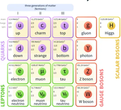
eight massless gluons. The existence of these vector bosons is the direct result of the SM gauge symmetries1. The Standard Model of elementary particles, with the three generations of matter, gauge bosons in the fourth column, and the Higgs boson in the fifth are shown on Figure 1.1.1.

Gauge invariance is the basic principle of the SM in which each interaction is de-scribed in a gauge theory. The Lie algebra of the local gauge transformations group completely determines the nature and properties of the interactions between parti-cles. The strong interaction is described by quantum chromodynamics (QCD) based on SU(3)C group, where C corresponds to the colour quantum number, quarks and

gluons are coloured objects, called partons; it is presented in Section 1.1.1. The elec-tromagnetic interaction and the weak interaction is represented by U(1)Y and SU(2)L

symmetry groups, where Y corresponds to hyper charge quantum number and L in-dicates that the coupling is only to left-handed fields. The electromagnetic and weak forces are unified to the electroweak theory, which is described in Section 1.1.2. The intensity of interactions between particles is quantified by the free parameters called couplings.

The requirement of the local gauge invariance of the Lagrangian forbids the bosonic and fermonic mass terms (will be shown later in the text), therefore all the particles are massless in the SM theory. The interaction with an extra field causes the symmetry to break, allowing mass terms and at the same time preserves the gauge invariance of the theory. The spontaneous symmetry breaking is realized by the Higgs mechanism in the electroweak theory; it will be discussed in Section 1.1.3. The Higgs boson acts as the mediator of a new class of interactions which, at the tree level, are coupled in

Figure 1.1.1: The particle content of the Standard Model, including the fermions (quarks and leptons), the gauge bosons, and the Higgs boson

proportion to the particle masses. The Higgs particle has now been observed at the LHC with mH ⇠ 125 GeV, thus making a big step towards completing the experimental

verification of the SM.

The SM is a renormalizable field theory, which means that the ultraviolet diver-gences that appear in loop diagrams can be eliminated by a suitable redefinition of the parameters already appearing in the bare Lagrangian: masses, couplings, and field normalizations.

1.1.1 Quantum chromo dynamics

The strong interaction, quantum chromodynamics (QCD), is a renormalizable gauge theory based on the group SU(3) with colour triplet quark matter fields [9, 10], described by the Lagrangian density:

L_{SU (3)} = 1 4 8 X A=1 FAµ⌫F_µ⌫A + nf X j=1 ¯ qj↵i /D↵q_j, (1.1)

here qj are the quark fields with nf di↵erent flavours, and Dµis the covariant derivative of the form: D↵_µ = @µ ↵ + igsGiµ i ↵ 2 , (1.2)

where gs is the QCD gauge coupling constant, ↵, =1,2,3 are colour indices. The

quarks transform according to the triplet representation matrices i/2. The ’s are the Gell-Mann SU(3) matrices, normalised by Tr i j = 2 ij The gluon field corresponds to Gi_µ, i = 1, ..., 8, and it enters the field strength tensor, describing the dynamics of the gluon field:

F_µ⌫i = @µGi⌫ @⌫Gµi gsfijkGjµGk⌫, (1.3)

the last term multiplies two gluon fields allows gluons to interact with each-other; the fijk(i, j, k = 1, ..., 8) are the structure functions defined by

[ i, j] = 2ifijk k (1.4)

The first term in 1.1 corresponds to three and four-point gluon self-interactions and the second to the quark interactions. QCD has the property of asymptotic freedom [11]: the coupling becomes weak at high energies or short distances (and accordingly increases at low energy/large distances). The strength of interaction between two partons in-creases with the relative distance, therefore it is not possible to observe a free parton but only color-neutral objects called hadrons. As soon as two coloured objects are pulled apart, the potential energy available will create new q ¯q pairs that neutralize the original quarks colours: this property is denoted as confinement[12]. Therefore, the decay products of the QCD process with quarks and gluons create flows of hadrons forming jets; these are the jets which are reconstructed in the detector. The dynamics of the QCD processes will be discussed in details in Section 1.2.

1.1.2 The electroweak interactions

The electromagnetic interaction describes the dynamics of the charged fermions, it is based on a local gauge transformation of the U(1) symmetry group [13], with the following properties:

• it describes the interaction of a charged particle with the photon; • the photon is massless (mass term is not gauge invariant);

• the gauge field does not have self-interactions.

The weak interaction is based on the SU(2) symmetry group, and the weak force is characterised by the following properties:

• it is capable of changing the flavour of quarks and leptons ; • it has massive force-carriers;

• it violates the parity transformation P, the charge symmetry C and the combined CP 1 _{symmetry [14].}

The maximal violation of C and P implies that the weak interaction to act di↵erently on fermions depending on the projection of the spin onto the momentum direction, and by that property they are split into left- and right-handed fermions, L and R

correspondingly. Under weak isospin SU(2) transformations the left-handed particles are weak-isospin doublets (I3 =±1₂), whereas the right-handed are singlets (I3 = 0)

-therefore the weak interaction only acts on left-handed fermion. This property implies that the right-handed neutrino is sterile, since it has no charge for any of the interactions described by the SM: no electric charge, no weak isospin, no colour.

The unification of the electromagnetic and weak interactions is presented by the electroweak theory, which is based on the SU(2)L⌦U(1)Y group gauge

transforma-tion. The SU(2)Lgroup is associated with the weak isospin I3and the gauge invariance

conditions introduces three gauge bosons W_µi, i = 1, 2, 3. The U(1)Y is associated with

the hypercharge Y and one gauge boson Bµ. The electromagnetic charge can be

re-lated to weak isospin and hypercharge through the relation Q = I3 +Y₂. Bµ couples

both to the left- and right-handed components of the fermion fields, the W_µi fields only couple to the left-handed fermions. The invariance under SU(2)L⌦U(1)Y is obtained

by the definition of two covariant derivatives, applied on left-handed and right-handed fermions in the Lagrangian describing the electroweak interaction:

Dµ,L= @µ+ ig i 2W i µ+ ig0 Y 2Bµ Dµ,R= @µ+ ig0Y 2Bµ (1.5)

The g and g0 coupling constants are the ones for SU(2)L and U(1)Y, respectively and i are the Pauli matrices. The Lagrangian of electroweak interaction can be presented

as the following: LEW = 1 4W i µ⌫Wµ⌫,i 1 4Bµ⌫B µ⌫_{+ i ¯} LD/L L+ i ¯RD/R R (1.6)

where the field strength tensors correspond to the kinematic of the bosons and are defined as:

Bµ⌫ = @µB⌫ @⌫Bµ

W_µ⌫i = @µW⌫i @⌫Wµi g✏ijkWµjW⌫k,

(1.7)

where ✏ijk are the group structure constants which for SU(2) coincides with the totally

antisymmetric Levi-Civita tensor, with ✏123= 1.

The physical bosons are linear combinations of the SU(2)L and U(1)Y fields. The

W+ and W are responsible for the charged current interactions :

W_µ±= p1 2(W

1

µ⌥ iWµ2) (1.8)

current interactions:

Aµ= Wµ3sin ✓W + Bµcos ✓W

Z_µ0= W_µ3cos ✓W Bµsin ✓W

(1.9)

where ✓W is the Weinberg angle which defines how the Bµ and Wµ3 rotate and mix to

form the observable Aµ, Zµ0 fields. The Weinberg angle can be expressed in terms of

the g and g0 coupling constants cos ✓W = p g g2_+g02.

Bosonic mass terms (1₂mXXµXµ) as well as fermionic mass terms (mi i i) would

break the local gauge invariance SU(2)L and U(1)Y. Therefore at this stage of the

Standard Model construction all the particles are massless. While the numerous ex-perimental evidences show that both fermions and bosons have a non-zero mass, a mechanism to introduce mass to the particles while preserving the local gauge invari-ance is provided by the spontaneous breaking of the symmetry.

1.1.3 Spontaneous symmetry breaking

The problem of the origin of the mass of quarks and leptons is solved by intro-ducing the Higgs-Brout-Englert-Guralnik-Hagen-Kibble mechanism [15, 16, 17]. The Higgs boson is a consequence of the electroweak symmetry breaking, which gives other particles mass through a dynamical mechanism - by introducing a new field. To give masses to the particle we define a complex SU(2)L doublet:

= p1 2 ✓ 1+ i 2 3+ i 4 ◆ = ✓ ₊ 0 ◆ , (1.10)

where + is a charged field with I3 = +1/2 and 0 is a neutral field with I3 = -1/2.

The Lagrangian to describe the dynamics of this field is written as:

L_{EW SB} = (Dµ )†(Dµ ) V ( ), (1.11)

where Dµ, the covariant derivative is given by: Dµ,L= (@µ+ig₂iWµi+ig0 Y2Bµ), is used

to ensure gauge invariance under U(1)Y⌦ SU(2)L. The symmetry breaking is obtained

through the form of the scalar potential V:

V ( ) = 1 2µ

2 † ₊1

4 (

† ₎2_{, (1.12)}

where it will be assumed that > 0, to ensure potential stability. The value of the potential V ( ) in the vacuum (no excitation) is obtained when @V_@ = 0, i.e. for:

µ2| | + | |3 = 0, (1.13)

i.e. when its module_{| | = 0 (if µ}2 _{> 0) or when| | = ±}q µ2

(if µ2_{< 0, the SU(2)} L

symmetry is broken only in this case).

state simply writes as: = p1 2 ✓ 0 ⌫ ◆ , (1.14)

This field has only a neutral and scalar component. This form of field explicitly breaks the SU(2)Linvariance (electroweak symmetry breaking, or EWSB). The

param-eter ⌫ is called the vacuum expectation value. The excitations from the ground state are given by:

= p1 2 ✓ 0 ⌫ + H(x) ◆ , (1.15)

where H is a physical scalar field, which quantum excitation is called the Higgs bo-son. This field gives rise to masses of the weak bosons W, Z - put field to term (Dµ )†(Dµ ), using definition of covariant derivative from 1.5 we obtain:

(Dµ )†(Dµ ) = ✓ @µ+ i 2g iW i µ+ i 2g 0_B µ ◆ 1 p 2 ✓ 0 ⌫ ◆ 2 = ⌫ 2 8 ⇣ g iWµi + g0Bµ⌘ ✓ 0₁ ◆ 2 = ⌫ 2 8 ✓ gW_µ1 igW_µ2 gW3 µ+ g0Bµ ◆ 2 = ⌫ 2 8  g2⇣(W_µ1)2+ (W_µ2)2⌘+ ( gW_µ3+ g0Bµ)2 (1.16)

If one use Equation 1.8, the term W_µ±W_±µ equal to the first term of Equation 1.16: (W_µ1)2+ (W_µ2)2. Using the Z from Equation 1.9 and notion for the Weinberg angle one get the second term of Equation 1.16:

Zµ= (Wµ3cos ✓W Bµsin ✓W) = 1 p g2_{+ g}02(gW 3 µ g0Bµ) (1.17)

Therefor, Equation 1.16 provides mass terms1 for the physical W± and Z0 bosons. The Aµ field quantum excitation does not gain mass, as no corresponding mass term

is found in the Lagrangian. The corresponding masses are:

m = 0, mZ = ⌫ 2 p g2_{+ g}02 mW = g⌫ 2 , mH = p 2µ2₌p_{2 ⌫}2 (1.18)

the Higgs boson obtains a mass through the same type of couplings. Since is a free parameter of the theory, the Higgs mass is not predicted by the SM.

To give masses to fermions we use the Higgs boson field to define Yukawa couplings

1 1

2mXXµX µ

yX (where X is a fermion) into the Lagrangian: L_d= yd( ¯L R) + h.c. = _p1 2yd⌫ ¯dLdR 1 p 2yd ¯ dLHdR+ h.c. (1.19)

where ydis the fermion Yukawa coupling which denotes the strength of the scalar field

coupling. The first term gives the mass of the down-type quark md= yd⌫/

p

2, while the second shows how fermions couple with strength ydto the Higgs field H. Since they

have right and left components, only the quarks and the charged leptons gain mass. A fermion X mass writes mX = yX⌫/

p

2. The neutrinos which are never observed to be right-handed are not given mass in the SM.

The U(1) symmetry and the SU(3) colour symmetry remain unbroken and therefore their carriers, photon and gluons, remain massless.

Standard Model summary

The SM describes the elementary particles and their interactions; it contains 19 free parameters that are necessary to describe the masses of the particles and the di↵erent couplings between the particles. Once the mass of the Higgs boson is measured, all the fundamental parameters of the Standard Model can be computed. This requires the precision measurement of the parameters of the Higgs boson, such as its mass and the couplings to fermions and bosons.

Figure 1.2.1: Schematic representation of a proton-proton hard scattering pro-cess [19].

1.2

Proton-proton interactions at LHC

Proton-proton collisions can be described by three types of interactions: elastic (⇠25 mb) when the incoming protons remain, di↵ractive (_{⇠10 mb) where the energy transfer} is low, and non-di↵ractive (_{⇠60 mb) when two partons from the protons interact with} a high momentum transfer. I shall describe the hard scattering interactions as it is main process via the Higgs boson or any new object would be produced. The ATLAS trigger selection is defined to select events produced by hard scattering processes. Hard scattering interactions are described by perturbative QCD. A schematic representation of a hard scattering proton-proton collision is given in Figure 1.2.1.

The hard scattering is accompanied by the interactions of the remanent partons from the proton, leading to extra activity around the objects produced by the hard scattering. This is called the Underlying Event (UE). Particles from the UE contribute to the triggered event (see Figure 1.2.2).

A second contribution, called pile-up, is superimposed to the hard scattering process at LHC. Because of the very high density of protons at the collision points, more than one proton interact when the two LHC proton bunches cross each other at the center of the experiment. For instance, the average number of interactions per bunch crossing (µ) was 23 during the 2016 data taking campaign. These pile-up events are essentially produced by soft processes and described by non-perturbative QCD e↵ects. Figure 1.2.3 shows an event display of Higgs candidate decaying to 2e2µ. The insert at the bottom shows the distribution of the 25 pile-up vertices measured by the ATLAS pixel detector.

Figure 1.2.2: Schematic representation of a proton-proton hard scattering and of the underlying event [20].

Figure 1.2.3: Event display of Higgs candidate decaying to 2e2µ [31]. The insert at the bottom shows the distribution of the 25 pile-up vertices measured by the ATLAS pixel detector.

1.2.1 Hard process

The LHC provides high energy proton-proton collisions at the energy of 6.5 TeV per beam. The factorisation theorem [21] states that hadron-hadron collision can be split into two parts: one describing structure of the hadron and interaction of the partons. Therefore the cross-section pp!X can be written as:

pp!X = PDFs⌦ hard scatter (1.20)

First term is denoted to the parton distribution functions (PDFs), they are uni-versal property of the incoming hadron, they do not depend on the hard scattering process. Parton distributions are not calculable in perturbative QCD and have to be obtained from experiment. The second term, the partonic cross section, is denoted as hard scattering, it can be computed as a perturbation series in ↵s and does not

depend on the type of incoming hadron.

pp!X =

X

q,q0

Z

dx1dx2fq(x1, Q2)fq0(x₂, Q2)⇥ ˆ_qq0_!X(x₁s, x₂s) _(1.21)

where x1 and x2 are the momentum fractions of the protons carried by the partons

q and q0 respectively and fq (fq0) represents the momentum fraction distribution of

a parton q (q0) which depends also on the four momentum of the process Q2_{. The}

partonic cross-section can be expressed as a power series expansion of the ↵s coupling

constant: ˆq ¯q!X = ˆ_|{z}0 LO + ↵_{| {z }}sˆ1 NLO + ↵_s2ˆ2 | {z } NNLO (1.22)

LO refers to the leading order, NLO to the next-to-leading order and NNLO to the next-to-next- to-leading order calculations. Figure 1.2.4 shows the predictions for some important Standard Model cross sections at p¯p and pp colliders, calculated at next-to-leading order in perturbation theory. The cross section of the QCD jet production has dominant contribution to the total cross section. The Higgs boson production cross section is about seven-eight orders of magnitude smaller then QCD jet production, three-four orders smaller than EW production of W and Z bosons and about two orders with respect to the top-quark production.

1.2.2 Parton density function

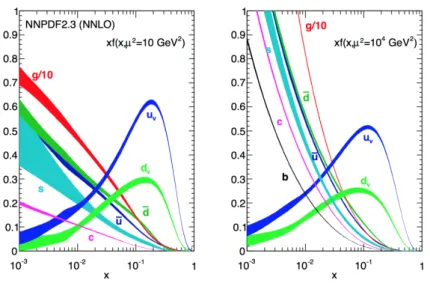
The parton distribution functions are defined as the probability of finding a parton in a proton with the momentum fraction x, at momentum transfer Q2. The set of distributions fi(x, Q2) describes how the momentum of the proton is shared between

the individual partons ( fi = valence quark, sea quarks and gluons). Figure 1.2.5

displays an example of xf (x, Q2_{) distributions for the valence quarks u and d, the sea}

quarks ¯u, ¯d, s, ¯s, b, ¯b and the gluon g for two di↵erent scales Q2 _{= 10 GeV}2 _{and 10}4

GeV2 _{. In most of the phase space the gluon PDF dominates.}

Dokshitzer-Figure 1.2.4: Main SM processes cross sections in hadronic collisions as a function ofps (center- of-mass energy) [28].

Gribov-Lipatov- Altarelli-Parisi (DGLAP) equations1. However, the PDFs themselves are not calculated perturbatively but are derived by fitting the experimental data in fixed target and collider experiments.

1.2.3 Hadronization and fragmentation

The scattering of the proton constituents leading to outgoing partons (quarks and gluons) with large transverse momenta. The partons are coloured objects and due to the confinement can’t propagate free, therefore additional q ¯q pairs will be created to build colourless hadrons. The flow of the hadrons will constitute ”jet” structure via a ”fragmentation process”. The process involves the production of hadrons and takes place at an energy scale where the QCD coupling constant is large and perturbation theory cannot be used. Fragmentation is therefore described using a QCD-motivated model with parameters that must be determined from experiment.

Figure 1.2.5: Parton distribution functions of the proton at next-to-leading order (NLO) for two di↵erent scales Q2 as predicted by the NNPDF collaboration. The band represents the 68% confidence level [29].

1.2.4 Monte Carlo generators

Monte Carlo generators produce complete events starting from a proton-proton initial state. They are used standalone or with specialized generators that improve the description of certain final states. They have many parameters, some of which are related to fundamental parameters such as the QCD coupling constant and electroweak parameters, and some of which describe the models used to parametrize long distance QCD, soft QCD, and electroweak processes.

Sherpa uses an interface to Pythia’s hadronization model and produces complete events [24]. It provides approximations for final states with large numbers of isolated jets. Sherpa generates underlying events using a simple multi-parton interaction model based on that of Pythia [25]. It can include high order LO matrix elements and also NLO computations for some processes. Sherpa allows to merge matrix elements with the parton-shower simulation [26], using di↵erent prescriptions (e.g. ME+PS@LO [27]) MC@NLO uses fundamental (hard scattering) processes evaluated at next to lead-ing order in QCD perturbation theory [30]. MC@NLO includes one loop corrections, with the consequence that events appear with negative and positive weight which must be taken into account when they are used. MC@NLO has been used for large-scale production of top, W and Z events.

1.3

Higgs physics at LHC

A new particle, with the properties consistent with the SM Higgs boson has been ob-served by the ATLAS and CMS collaborations in the mass region around 126 GeV [105, 106]. In this section, the Higgs boson production and decay modes will be discussed. The properties of the recently observed Higgs boson will be presented. The review of the parameters of the SM will be presented, comparing predicted and measured values.

1.3.1 Higgs boson production

At the LHC, the SM Higgs boson is produced in proton-proton collisions through four dominant processes: gluon gluon fusion (ggF ), vector boson fusion (VBF ), associ-ated production with a W or Z boson (VH ), or associassoci-ated production with a pair of top quarks(t¯tH). The Feynman diagrams of the processes are presented on Figure 1.3.1.

• The Higgs boson cannot couple directly to massless gluons, therefore the process is mediated by triangular loops of heavy quarks. The gluon-gluon interaction is the leading production process in pp collisions since gluons has the largest contribution in the parton density function, therefore the ggF process has largest contribution in the Higgs production. Cross sections of the ggF process are calculated at N3LO QCD and NLO EW accuracies [33].

• The VBF has the second largest cross section at the LHC. It has distinguish-able signature in the detector with two high pT jets which can be exploited at

the LHC to discriminate the VBF signal against backgrounds and other signals. The VBF cross sections are calculated at (approx.) NNLO QCD and NLO EW accuracies [34, 35].

• The associated production (VH ) corresponds to the process when the Higgs boson is radiated from an o↵-shell W± or Z weak boson from quark-antiquark annihilation. The decay products of the associated bosons (presence of lepton(s) and/or missing transverse energy) are used to tag the event. Cross sections of the VH are calculated at NNLO QCD and NLO EW accuracies [36].

• The associated production with a pair of top-quarks (ttH ) process is similar to the gluon gluon fusion process. It has the smallest cross section, an order of magnitude smaller than ggF due to the presence of two real top-quarks in the final state. The top decays lead to high jet multiplicity in the final state, leptons and transverse missing energy, which makes this production mode challenging to explore due to low signal over background ratio. Cross sections of the ttH are calculated at NLO QCD and NLO EW accuracies [37].

Values of the cross section for each process for the Higgs boson at ps =13 TeV as a function of mass are presented on Figure 1.3.2 (left).

Figure 1.3.1: Leading-order Feynman diagrams of the four main SM Higgs boson production processes with the fraction of the contribution to the total cross section. (a) gluon gluon fusion. (b) Vector Boson Fusion. (c) associated production with a vector boson. (d) associated production with a pair of top quarks.

1.3.2 Higgs boson decay channels

The Higgs boson can decay to several channels. The branching fractions are cal-culated through the computation of all the partial decay widths in the HDecay [41] and Prophecy [42] programs, including all kinematically allowed channels and all rel-evant higher-order QCD corrections to decays into quark pairs and into gluons. The branching fractions (BRs), as a function of the Higgs boson mass, are represented in Figure 1.3.2 (right) for the relevant decay modes.

The Higgs boson decays mainly to pairs of b- and c-quarks, pairs of W and Z bosons, pair of gluons and ⌧ ⌧ . Those processes has largest production rate, the final states are composed of hadronic jets from quarks and the decay products of the bosons. The diphoton channel has a considerably lower branching fraction than the other channels, but it is actual final state. For example, the branching fraction to diphoton is 2.27⇥ 10 3_{, while the branching fraction to ZZ is one order magnitude larger,}

2.619⇥ 10 2_{. To obtain the rate of ZZ ! 4e one needs to take into account the}

Z decay fraction to electrons, which is 3.36⇥ 10 2 _{for each of the Z. Therefore,}

comparing the rate of diphoton events to the one of the channel with four electrons one gets 2.27_{⇥ 10} 3 _{versus 2.95⇥ 10} 5_{. Despite the fact that the is mass-less, the}

H _! decays is possible via loop diagrams containing massive charged particles like W±, b and t - since the Higgs couplings to fermions is proportional to the mass, contribution of light fermions to the loop are neglected. The Feynman diagrams for the Higgs boson decays to a pair of photons are presented on Figure 1.3.3.

The diphoton channel played a crucial role in the discovery of the Higgs boson. This decay process will be used for search for new scalar resonances. This search is described in details in Chapter 5.

1.3.3 Higgs boson discovery and success of the Standard Model

The Higgs boson, which was predicted in 1964, has been discovered at the LHC in 2012 by the ATLAS and CMS collaborations. The measurements of the Higgs boson

[GeV] H M 120 122 124 126 128 130 H+X) [pb] → (pp σ 1 − 10 1 10 2 10 _{s= 13 TeV} LHC HIGGS XS WG 2016

H (N3LO QCD + NLO EW) →

pp

qqH (NNLO QCD + NLO EW) →

pp

WH (NNLO QCD + NLO EW) →

pp

ZH (NNLO QCD + NLO EW) →

pp

ttH (NLO QCD + NLO EW) → pp bbH (NNLO QCD in 5FS, NLO QCD in 4FS) → pp tH (NLO QCD) → pp [GeV] H M 120 121 122 123 124 125 126 127 128 129 130 Hi g gs B R + T ot al Un ce rt -4 10 -3 10 -2 10 -1 10 1 LHC HIGGS XS WG 2013 b b τ τ µ µ c c gg γ γ ZZ WW γ Z

Figure 1.3.2: Standard Model Higgs boson production cross sections atps = 13 TeV (left) and decay branching ratios (right) [39].

Figure 1.3.3: Examples of leading-order Feynman diagrams for Higgs boson de-cays to a pair of photons.

mass in the diphoton and ZZ decaying to four leptons channels corresponds to mH

= 125.09_{±0.21(stat.)±0.11(syst) GeV with the full combined Run-1 dataset of two} experiments and the combination presented on Figure 1.3.4 [43].

The SM has been successfully tested at an impressive level of accuracy and pro-vides at present our best fundamental understanding of the phenomenology of particle physics. Various experimental facilities (LEP, Tevatron, LHC) have allowed us to mea-sure the parameters of the Standard Model with incredible precision, as it is summarised in Table 1.3.1. Figure 1.3.5 (left) shows agreement of the parameters with the data. The measured couplings of the Higgs boson to fermions and bosons are in excellent agreement with the behaviour expected in the SM, as shown on Figure 1.3.5 (right).

Figure 1.3.4: Summary of Higgs boson mass measurements from the individual analyses of ATLAS and CMS and from the combined analysis H _! and H _! ZZ! 4l [43].

Quantity Measurement [GeV] Standard Model Predictions [GeV] Pull, [ ]

mt 173.34 ± 0.81 173.76 ± 0.76 -0.5

MW 80.387 ± 0.016 80.361 ± 0.006 1.6

W 2.046 ± 0.049 2.089± 0.001 -0.9

MZ 91.1876± 0.0021 91.1880 ± 0.0020 -0.2

Z 2.4952 ± 0.0023 2.4943± 0.0008 0.4

Table 1.3.1: The measurements of the Standard Model parameters, compared to the predicted values, where pull is the deviation of the measured values from predicted in terms of standard deviations [44].

Figure 1.3.5: Success of the Standard Model. Left: summary of the measured parameters of the model (W, Z, H bosons, top quark) and their dependence on the Higgs boson (MH) and top quark (mt) masses [44]. Right: Best fit values of

the couplings of fermions (Fm_⌫F) and the weak bosons (pVm_⌫V) as a function of

particle mass for the combination of ATLAS and CMS data, where ⌫ = 246 GeV is the vacuum expectation value of the Higgs field. The dashed (blue) line indicates the predicted dependence on the particle mass in the case of the SM Higgs boson. The solid (red) line indicates the best fit result to the [M, "] phenomenological model with the corresponding 68% and 95% CL bands [45].

1.4

Beyond Standard Model

Despite the fact that the SM is a very successful theory, describing particle physics phenomena at energies up to the TeV scale, and supported by all experimental observa-tions, it still has open questions in the description of Nature. The SM does not explain the gravitational force and it does not provide candidates for the dark matter and in-visible energy inferred by cosmological observations. Matter-antimatter asymmetry in the universe is unexplained.

Several new physics extensions attempt to account for these observations. Examples of extensions are supersymmetry, where each SM particle is endowed with a superpart-ner, or extra dimensions, where one or several extra spatial dimensions are added to the already existing three. The Minimal Supersymmetric Standard Model (MSSM) con-tains two Higgs doublets model and it is one of the simplest possible extensions of the SM. The MSSM predicts additional scalar particles with the similar properties as the Higgs boson. An introduction will be presented in Section 1.4.1. The original proposal for extra dimensions by Kaluza and Klein where attempts to unify electromagnetism with gravitation, will be briefly discussed in Section 1.4.2.

1.4.1 Two Higgs Doublet Model

The Two Higgs Doublet Mode (2HDM) model is a simple extension of Standard Model, where an additional Higgs doublet is added [1, 3, 4]. One of the motivations for the 2HDMs is that it can generate a baryon asymmetry in the Universe, due to the flexibility of their scalar mass spectrum and the existence of additional sources of CP violation. There has been many works on baryogenesis in the 2HDM [46].

In theories with two Higgs doublets, the Yukawa couplings are:

VY ukawa =

X

i=1,2

(Q iyiuu + Q¯ iyidd + L¯ iyei¯e + h.c.), (1.23)

where yu

i (yid) corresponds to couplings for up-type (down-type) quarks and yie is

cou-plings for charged leptons.

In the 2HDM the flavour-changing neutral currents (FCNC) are allowed at tree level, which creates a potential problem of the model, since FCNC are not observed [5]. Depending on which type of fermions couples to which doublet (by convention up-type quarks are always taken to couple to 2), one can divide two-Higgs-doublet models

into the following tupes:

• Type I: in which y1u,d,e = 0; all fermions couple to one doublet.

• Type II: in which yu

1 = yd2 = y2e = 0; the up-type quarks couple to one doublet

and the down-type quarks and leptons couple to the other.

• Type III: in which yu1 = yd1 = y2e = 0; quarks couple to one doublet and leptons

• Type IV: in which yu

1 = ye1 = y2d = 0; up-type quarks and leptons couple to one

doublet and down-type quarks couple to the other.

In the following, in order to avoid FCNC, only the types I and II are considered. This is achieved by imposing a discrete or continuous symmetry. For instance, for the Type-I 2HDM model, one assumes the symmetry of type 1! 1, where all fermions

with same quantum numbers couples to the same Higgs multiplet; in that case FCNC is absent. Also, it is assumed that CP is conserved to distinguish between scalars and pseudoscalars.

Exploiting the SM mathematical framework described in Section 1.1, we introduce a new potential V ( ) similarly to the one used in Equation 1.12. The most general scalar potential for two doublets 1 and 2 with hypercharge +1 is:

V ( ) =m2₁₁ †₁ 1+ m222 †2 2 m212( †1 2+ †2 1) + 1 2 ( † 1 1)2+ 2 2 ( † 2 2)2 + 3 †1 1 †2 2+ 4 †1 2 †2 1+ 5 h ( †₁ 2)2+ †2 1)2 i , (1.24)

where m2₁₂ and k, k = 1...5 (Higgs self-couplings) are free and real parameters.

For a region of parameter space, the minimization of this potential gives

h 1i0= 0 ⌫1 p 2 ! ,_h 2i0 = 0 ⌫2 p 2 ! , tan _⌘ ⌫2 ⌫1 (1.25)

The angle is the rotation angle which diagonalizes the mass-squared matrices of the charged scalars and of the pseudoscalars. The angle ↵ is defined to be the rotation angle which diagonalizes the mass-squared matrix of the CP even neutral scalars.

With two complex scalar SU(2) doublets there are eight fields:

a= ✓ _† a (⌫a+ ⇢a+ i⌘a)/ p 2 ◆ , a = 1, 2. (1.26)

Three of those gives mass to the W± and Z0 _{gauge bosons; the remaining five are}

physical scalar (”Higgs”) fields. There is: • the CP even neutral scalars h and H • the CP odd pseudoscalar A

• and two charged Higgs bosons H±

The two parameters ↵ and determine the interactions of the various Higgs fields with the vector bosons and (given the fermion masses) with the fermions; they are thus crucial in discussing phenomenology. Those parameters are the rotational angles which diagonalize the mass-squared matrices of the scalars.

The vacum expectation values (vev) of the doublets from Equation 1.26 can be expressed as ⌫1 = ⌫ cos , ⌫2 = ⌫ sin and

p ⌫2

2HDM I 2HDM II

hV V sin ( ↵) sin ( ↵)

hQu cos ↵/ sin cos ↵/ sin hQd cos ↵/ sin sin ↵/ cos hLe cos ↵/ sin sin ↵/ cos

HV V cos ( ↵) cos ( ↵)

HQu sin ↵/ sin sin ↵/ sin HQd sin ↵/ sin cos ↵/ cos HLe sin ↵/ sin cos ↵/ cos

Table 1.4.1: The tree-level couplings of the neutral Higgs bosons h and H to up- and down-type quarks, leptons, and massive gauge bosons relative to the SM Higgs boson couplings as func-tions of ↵ and in the two types of 2HDM [7]. 2HDM I 2HDM II hV V 1 1 hQu 1 1 hQd 1 1 hLe 1 1 HV V 0 0

HQu -1/tan -1/tan

HQd -1/tan tan

HLe -1/tan tan

Table 1.4.2: The tree-level couplings of the neutral Higgs bosons h and H to up- and down-type quarks, leptons, and massive gauge bosons relative to the SM Higgs boson couplings as functions of ↵ and in the two types of 2HDM in case of alignment limit ( ↵ = ⇡/2).

scalars are a lighter h and a heavier H, which are orthogonal combinations of ⇢1 and

⇢2:

h = ⇢1sin ↵ ⇢2cos ↵,

H = ⇢1cos ↵ ⇢2sin ↵.

(1.27)

the Standard-Model Higgs boson would be:

hSM = ⇢1cos ↵ + ⇢2sin ↵,

= h sin ( ↵) H cos ( ↵). (1.28)

The coupling of the light Higgs, h, to either W W or ZZ is the same as the Standard-Model coupling times sin ( ↵) and the coupling of the heavier Higgs, H, is the same as the Standard-Model coupling times cos ( ↵), as presented in Table 1.4.1. Therefore, in case when cos ( ↵) = 0, the so-called alignment limit, the lighter CP even h has couplings like the Higgs boson of the Standard Model, as shown in Table 1.4.2.

Diphoton resonances

Searches for heavy scalar (H) in diphoton channel in general are suppressed by large partial decay widths into W W , ZZ and t¯t. The coupling values of the second boson to the SM particles are constrained by the resonance already observed at 125 GeV. This allows to probe alignment limit of the 2HDM-type models, where the couplings of the second scalar particle to the V V are suppressed, as shown in Table 1.4.2. Under these assumptions, the second resonance is expected to have sizeable branching fractions in the final states through the up-type quarks loops [5]. In the 2HDM Type-II model

for low values of tan parameter the decay modes to bottom-type quarks (b¯b) and leptons (⌧ ⌧ ) are suppressed with respect to . This enhancement of diphoton decay channel is valid up to t¯t threshold, above which the t¯t decay mode should become dominant.

In 2015 the LHC resumed operation after a long shutdown of two years. The centre of mass energy had increased from 8 to 13 TeV, opening a new phase space to search for new resonances. As part of my PhD, I searched for a new resonance decaying to a pair of photons, as described in Chapter 5.

1.4.2 Extra dimension theory

One of the questions unsolved in the SM, is the so called ”hierarchy problem”: why the gravity is so weak (the weak force is 1024 times as strong as gravity)? Extra dimensions are proposing additional space or time dimensions beyond the standard (3 + 1) typical of our observed space-time, to solve the this problem, and were introduced in the Kaluza-Klein theory.

Figure 1.4.1: Cartoon of the RS scenario with a brane-localized SM. The warp factor, (R/z)2_{, causes energy scales to be scaled down towards the TeV brane [48].}

Warped extra dimensions, such as those proposed by the Randall-Sundrum model (RS) [47], introduce separation of two 4-D hypersurfaces (branes) by a small extra (5th) dimension. In their original model, our universe lives on one brane, the ”TeV brane” with negative energy density, the fields of the Standard Model are generally confined to this brane. There exists a second, ”Planck brane” of positive energy density sep-arated by the extra dimension, as shown on Figure 1.4.1. The energy density of the branes warps the space-time in the 5-D bulk. This causes gravity which is a weak force

corresponding to a high mass scale on the TeV brane to become a strong force corre-sponding to a low mass scale on the Planck brane. Given this space-time configuration, TeV scales are naturally generated from the Planck scale due to a geometric ”warp” factor that relates the fundamental Planck scale on one brane to the apparent scale on the other with a coupling scale ⇤⇡ defined as:

⇤⇡ = MPl exp( k⇡rc) (1.29)

where MPl = MPl/

p

8⇡ is the reduced Planck scale, and k and rc are the curvature

and compactification radius of the extra dimension, respectively. This e↵ectively solves the hierarchy problem and predicts that there should be exotic TeV-scale spin 2 states (Kaluza-Klein or KK gravitons). In the minimal RS model, gravitons are the only particles that can propagate in the bulk. These KK gravitons should have spin 2, a mass splitting between successive KK levels on the TeV scale, and a universal dimensionless coupling k/MPl to the SM fields. A striking signature of the RS model at hadron

colliders would be graviton production [49], followed by their decay to pairs of SM fermions or bosons. The decay G⇤ _! is a particularly interesting example, since observation of a resonance in the diphoton final state would rule out some possible interpretations, such as a Z0 boson.

The search for the graviton decaying to pair of photons has been performed by the ATLAS collaboration [116], using the same dataset used for the search for scalar resonance presented in Chapter 5. Di↵erent kinematic selections and treatment of the background with respect to spin-0 analysis are introduced. No significant deviation from the Standard Model background-only hypothesis is observed. Upper limits on the spin-2 RS graviton cross section times branching ratio to two photons as a function of the mass and coupling k/MPl are set.

The LHC and the ATLAS

Detector

Contents

2.1 The Large Hadron Collider (LHC) . . . 31

2.1.1 LHC Machine . . . 31

2.1.2 LHC layout and beam facility . . . 31

2.1.3 LHC magnets . . . 32

2.1.4 LHC performance . . . 33

2.1.5 The LHC upgrade plan . . . 36

2.2 ATLAS Detector . . . 39

2.2.1 Inner Detectors . . . 39

2.2.2 Calorimeters . . . 43

2.2.3 Muon System . . . 45

2.2.4 Trigger System . . . 47

2.3 The Liquid Argon Calorimeter . . . 50

2.3.1 Electromagnetic shower development . . . 50

2.3.2 Calorimeter structure . . . 51

2.3.3 Energy resolution of the electromagnetic calorimeter . . . 53

2.3.4 Calorimeter read-out structure . . . 54

2.3.5 Event format and bytestream . . . 60

2.4.1 Simulation . . . 63

2.4.2 Pileup Reweighting . . . 64

The ATLAS experiment is one of the four majour experiments at the Large Hadron Collider (LHC) at CERN. It is a general-purpose particle physics experiment run by an international collaboration involving more than 3000 physicists from 182 institutions of 38 countries. It is designed to exploit the full discovery potential and the huge range of physics opportunities that the LHC provides.

The structure of LHC machine and its performance will be discussed in Section 2.1. The description of ATLAS detector with a brief presentation of the subsystems and their role are presented in Section 2.2. A more detailed overview of the Liquid Argon (LAr) Electromagnetic calorimeter, its performance and read-out electronics are summarised in Sections 2.3.2, 2.3.3 and 2.3.4 correspondingly. The description of the general format of the data stream (Event Format) and my contribution to the tool to access and decode the raw data stream is given in Section 2.3.5. Section 2.4 is devoted to the description of the Monte Carlo simulation of the ATLAS detector and of the proton-proton physics precesses.

2.1

The Large Hadron Collider (LHC)

2.1.1 LHC Machine

The Large Hadron Collider (LHC) is the world’s largest instrument for Particle Physics research. It is a two-ring-superconducting-hadron accelerator, designed for proton-proton collisions at the center-of-mass energy ps = 14 TeV with an instanta-neous luminosity of 1034 _cm 2_s 1 _{and for heavy ions (Pb) collisions with an energy of}

2.8 TeV per nucleon and a luminosity up to 1027 _cm 2_s 1_{. The LHC is located near}

Geneva in a 27 kilometer circular tunnel, about 100 meters below ground level. The tunnel has eight straight sections, 528 m long each for experimental or utility insertions (denoted as Points), and eight arcs 2.45 km each containing the magnet system.

The LHC has performed very well; in following sections I will briefly describe the key elements of the collider for accelerating and steering the beams. The high performance accelerating cavities are used to push the beam and the magnetic field at the limit of technology - to bend the protons around the ring. Each of the parts of LHC is state of the art, technical details can be found in reference [50, 51].

2.1.2 LHC layout and beam facility

To produce collisions in the center of the LHC detectors, the two beams follow a long path through the accelerating complex, as it is presented on Figure 2.1.1. The protons are first produced by ionising hydrogen; the resulting protons are first accelerated to an energy of 750 keV. They are further accelerated in a linear accelerator, LINAC 2, to an energy of 50 MeV. The protons are split into four parts and injected into the Proton Synchrotron Booster (PSB), a 4-layer ring which accelerates them up to an energy of 1.4 GeV. In the Proton Synchrotron (PS) circular accelerator, the protons are collected to form bunches which are brought to an energy to 26 GeV. Bunches are injected to the Super Proton Synchrotron (SPS), where they are accelerated to an energy of 450 GeV. At that point, bunches are prepared for the LHC ring. Each proton gains 485 keV in one turn, and continue to ramp up to operating energy - 6.5 TeV per beam. The two beams at full intensity will consist of 2808 bunches, each of them containing 1.15_⇥1011 _protons.

The layout of LHC consists of four experimental and four utility insertions, as shown on Figure 2.1.2. The two high luminosity experiments, ATLAS [56] and CMS [57], are located at diametrically opposite straight sections, Point 1 and 5 respectively. Two more experimental insertions, caverns of ALICE [58] and LHCb [59] detectors, are located at Point 2 and Point 8, which also include the injection systems. The beams travel in opposite directions in an ultrahigh vacuum inside two separate beam pipes, Beam 1 is injected clockwise at Point 2 and Beam 2 is injected anti clockwise at Point 8. The two beams, which are share the same vacuum chamber, are squeezed and guided to the interaction point, as shown on Figure 2.1.3.

The collimation systems are important to provide stable, uniform and focused beams. Particles with a large momentum o↵set are scattered by the primary collimator (sequence of quadrupoles and dipoles) in Point 3, and particles with a large betatron