HAL Id: hal-01457986
https://hal.archives-ouvertes.fr/hal-01457986
Submitted on 6 Feb 2017
HAL is a multi-disciplinary open access
archive for the deposit and dissemination of
sci-entific research documents, whether they are
pub-lished or not. The documents may come from
teaching and research institutions in France or
abroad, or from public or private research centers.
L’archive ouverte pluridisciplinaire HAL, est
destinée au dépôt et à la diffusion de documents
scientifiques de niveau recherche, publiés ou non,
émanant des établissements d’enseignement et de
recherche français ou étrangers, des laboratoires
publics ou privés.
On the bend-number of planar and outerplanar graphs
Daniel Heldt, Kolja Knauer, Torsten Ueckerdt
To cite this version:
Daniel Heldt, Kolja Knauer, Torsten Ueckerdt. On the bend-number of planar and outerplanar graphs.
Discrete Applied Mathematics, Elsevier, 2014. �hal-01457986�
On the bend-number of planar and outerplanar
graphs
Daniel Heldt1, Kolja Knauer1, and Torsten Ueckerdt2
1
TU Berlin, Berlin, Germany
[email protected], [email protected]
2
Charles University in Prague, Prague, Czech Republic [email protected]
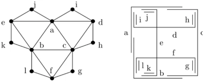
Abstract. The bend-number b(G) of a graph G is the minimum k such that G may be represented as the edge intersection graph of a set of grid paths with at most k bends. We confirm a conjecture of Biedl and Stern showing that the maximum bend-number of outerplanar graphs is 2. Moreover we improve the formerly known lower and upper bound for the maximum bend-number of planar graphs from 2 and 5 to 3 and 4, respectively.
1
Introduction
In 2007 Golumbic, Lipshteyn and Stern defined an EPG3 representation of a
simple graph G as an assignment of paths in the rectangular plane grid to the vertices of G, such that two vertices are adjacent if and only if the corresponding paths intersect in at least one grid edge, see [9]. EPG representations arise from VLSI grid layout problems [4] and as generalizations of edge-intersection graphs of paths on degree 4 trees [8]. In the same paper Golumbic et al. show that every graph has an EPG representation and propose to restrict the number of bends per path in the representation. There has been some work related to this, see [1, 2, 9, 13, 18]. A graph is a k-bend graph if it has an EPG representation, where
a a b b c c d d e e f f g g h h i i j j k k l l
Fig. 1. A 2-bend graph and an EPG representation. If a grid edge is shared by several paths we draw them close to each other.
3
each path has at most k bends. The bend-number b(G) of G is the minimum k, such that G is a k-bend graph.
Note that the class of 0-bend graphs coincides with the well-known class of interval graphs, i.e., intersection graphs of intervals on a real line. It is thus natural to view k-bend graphs as an extension of the concept of interval graphs and the bend-number as a measure of how far a graph is from being an interval-graph.
Intersection graphs of systems of intervals together with a parameter counting how many intervals are needed to represent a vertex of a given graph G have re-ceived some attention. Popular examples are the interval-number, see Harary and Trotter [12] and the track-number, see Gy´arf´as and West [11]. Extremal ques-tions for these parameters like ‘What is the maximum interval-/track-number among all graphs of a particular graph class?’ have been of strong interest in the literature. Scheinermann and West [19] show that the maximum interval-number of outerplanar graphs is 2 and of planar graphs is 3. Kostochka and West [15] prove that the maximum track-number of outerplanar graphs is 2 and Gon¸calves and Ochem [10] prove that the maximum track-number of planar graphs is 4. In [2] Biedl and Stern show that outerplanar graphs are 3-bend graphs and provide an outerplanar graph which has bend-number 2, see Fig. 1. They con-jecture that all outerplanar graphs are 2-bend graphs. We confirm this concon-jecture in Theorem 1, showing the stronger result that graphs of treewidth at most 2 are 2-bend graphs.
The major part of this paper is devoted to planar graphs. Biedl and Stern [2] show that planar graphs are 5-bend graphs but the only lower bound that they have is 2, given by the graph of Fig. 1. In Proposition 1 we provide a planar graph of treewidth 3 which has bend-number 3, thus improving the lower bound of the class of planar graphs by one. Indeed in Theorem 2 we show that every planar graph with treewidth 3 is a 3-bend graph. The main result of this article is Theorem 3. We improve the upper bound for the bend-number of general planar graphs from 5 to 4.
2
Preliminaries
We consider simple undirected graphs G with vertex set V (G) as well as edge set E(G). An EPG representation is a set of finite paths {P (u) | u ∈ V (G)}, which consist of consecutive edges of the rectangular grid in the plane. These paths are not self-intersecting (in grid edges), and P (u) ∩ P (v) 6= ∅ if and only if {u, v} ∈ E(G), i.e., only intersections at grid edges are considered. A bend of P(u) is either a horizontal grid edge followed by a vertical one or a vertical edge followed by a horizontal one in P (u).
Let us now introduce some terminology: The grid edges between two consecutive bends (or the first (last) bend and the start (end) of P (u)) are called segments. So a k-bend path consists of k + 1 segments, each of which is either horizontal or vertical. A sub-segment is a connected subset of a segment. In an EPG
rep-resentation a set of sub-segments (eventually from different segments) is called a part.
Furthermore, a vertex u is displayed, if there is at least one grid edge, which is exclusively in P (u) and in no other path. We then say that this grid edge is a private edge of P (u). An edge {u, v} ∈ E is displayed, if there is at least one grid edge in P (u) ∩ P (v), which is only contained in P (u) ∩ P (v) and not element of any other path. This grid edge is then called a private edge of P (u) ∩ P (v). We also say that a part (or sub-segment) displays the corresponding vertex or edge if it consists only of grid edges which are private edges of the respective vertex or edge.
Finally, two horizontal sub-segments in an EPG representation see each other if there is a vertical grid line crossing both sub-segments. Similarly, two vertical sub-segments see each other if there is a horizontal grid line crossing both.
3
EPG representations of graphs in terms of treewidth
In this section we consider graphs of bounded treewidth. Therefore we denote the treewidth of a graph G with tw(G) and make use of the fact, that every graph Gwith tw(G) ≤ k is a subgraph of a k-tree as well as the fact, that every k-tree admits a construction sequence, starting with a (k + 1)-clique and iteratively stacking a new vertices into k–cliques. For further definitions and more about construction sequences of graphs of bounded treewidth we refer to [3].
Theorem 1. For every graph G with tw(G) ≤ 2 we have b(G) ≤ 2.
Proof. Let ˜Gbe the 2-tree which contains G and (v1, . . . , vn) be a vertex ordering
of G implied by ˜G’s construction sequence. We construct a 2-bend representation of G along the building sequence G2 ⊂ . . . ⊂ Gn = G, where we add vertex vi
to Gi, such that the two neighbors of vi in ˜Gi form a 2-clique in ˜Gi (and not
necessarily in Gi). We maintain that Γi is a 2-bend representation of Gi, such
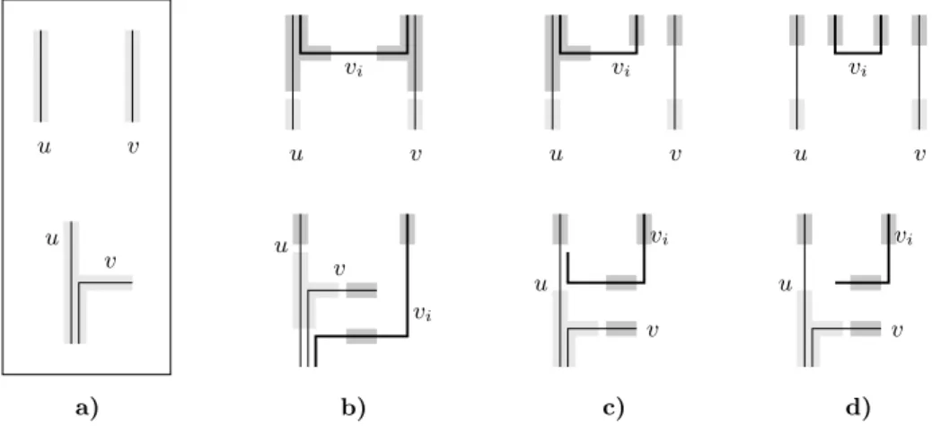
that every 2-clique in ˜Gi satisfies one of the two invariants in Fig. 2 a), i.e., for
i = 2, . . . , n and {u, v} ∈ E( ˜Gi) we have a sub-segment pu ⊆ P (u) and a part
pv⊆ P (v) such that one of the following sets of conditions holds:
(i) pv is a sub-segment, puand pvsee each other, pudisplays u, and pvdisplays
vas depicted in the top row of Fig. 2 a),
(ii) pv consists of two consecutive sub-segments pv,1, pv,2 such that there is a
bend between them, pv,2displays v, pu\pv,1displays u, and pu∩pv,1displays
{u, v} as depicted in the bottom row of Fig. 2 a).
The two possible starting representations for G2 are shown in Fig. 2 a). Now for
i≥ 2, let Γi be a 2-bend representation of Gi that satisfies our invariant.
Let {u, v} be the 2-clique that is the neighborhood of vi in ˜Gi. If vi has an
edge in Gi+1 with both, u and v, we introduce the path for vi as illustrated in
Fig. 2 b) depending on the type of the invariant for {u, v}. The parts, displaying the new 2-cliques {u, vi} and {v, vi} in ˜Gi+1, are highlighted in dark gray and
u u u u u u u u v v v v v v v v a) b) c) d) vi vi vi vi vi vi
Fig. 2. Invariants for a 2-clique and insertion rules for the path for the new vertex vi
(drawn bold). a) puand pvfor the two types of the invariant. b) Vertex vihas an edge
with both, u and v. c): Vertex vi has an edge with u and no edge with v. d): Vertex
vihas no edge with u or v.
If vi has an edge in Gi+1 with u and no edge in Gi+1 with v, we introduce the
path for vias illustrated in Fig. 2 c) depending on the type of invariant we have.
Again the parts, which display the new 2-cliques {u, vi} and {v, vi}, and the old
2-clique {u, v} in ˜Gi+1are highlighted in dark gray, and light gray, respectively.
If vihas an edge in Gi+1with v and no edge in Gi+1 with u, the roles of u and v
are basically exchanged. In case, vineither has an edge in Gi+1 with u nor with
v, we introduce the path for vi as illustrated in Fig. 2 d) depending on the type
of type of invariant for {u, v}. ut
Since every outerplanar graph G has a treewidth ≤ 2 we obtain the following corollary.
Corollary 1. For every outerplanar graph G we have b(G) ≤ 2.
This confirms a conjecture of Biedl and Stern [2], who show that the graph in Fig. 1 has no 1-bend representation. Therefore this bound cannot be further improved.
Theorem 2. For every planar graph G with tw(G) ≤ 3 we have b(G) ≤ 3. Proof. By a result of El-Mallah and Colbourn [6] G is a subgraph of a plane 3-tree ˜G. So there is a vertex ordering (v1, . . . , vn), such that ˜G3 is a triangle
{v1, v2, v3} and ˜Gi is obtained from ˜Gi−1 by connecting vito the three vertices
u, v, w of a triangle bounding an inner face of ˜Gi−1. The triangle {u, v, w} is
then not bounding an inner face of ˜Gi anymore and hence no second vertex may
be attached to it. We build a 3-bend representation of G concurrently with the building sequence G3 ⊂ · · · ⊂ Gn of G w.r.t. the vertex ordering (v1, . . . , vn).
We maintain the following invariant on the 3-bend representation Γi of Gi, for
(a) Every vertex u ∈ Γi has a horizontal and a vertical sub-segment displaying
u, and
(b) every facial triangle {u, v, w} of ˜Gi has two vertices, say u and v, of one of
the following two types:
(i) there is a sub-segment, which displays the edge {u, v} as in the left example in Fig. 3 a),
(ii) there is an entire segment s of P (v) displaying v and a sub-segment of P(u) displaying u and crossing s, see Fig. 3 a).
Moreover, we require that all the displaying parts above are pairwise disjoint and that the entire segment in every cross in (ii) cannot see displaying parts from (a). However, we need this assumption only in the case in Fig. 3 c).
u u u u u v v v v v v v v w w w w w vi vi vi vi vi
a) invariants for {u, v} of type (i) and (ii)
b) degGi(vi) = 3,
{u, v} of first type
c) degGi(vi) = 3,
{u, v} of second type
d) degGi(vi) = 2 e) degGi(vi) = 1 f ) degGi(vi) = 0
or or
Fig. 3. Building a 3-bend representation of a planar graph with tree-width 3, a vertex viis attached to the facial triangle {u, v, w} in ˜Gi−1 : In a) the two types of invariant
for {u, v} are shown. In b)–f ) it is shown how to insert the new vertex vi(drawn bold)
depending on its degree in Giand the invariant of {u, v}. The invariants for the three
new facial triangles {u, v, vi}, {u, vi, w}, and {vi, v, w} in ˜Giare highlighted.
It is not difficult to find a 3-bend representation Γ3 of the subgraph G3 of G,
which satisfies invariant (a) and (b). Indeed, by introducing three artificial outer vertices we can assume w.l.o.g. that G3 is an independent set of size three.
For i ≥ 4, the path for vertex vi is introduced to Γi−1 according to the degree
of vi in Gi and the type of invariant for the facial triangle {u, v, w} in ˜Gi−1
that vi is connected to. Fig. 3 b)–f ) shows all five cases and how to introduce
vi, which is illustrated by the bold path. Consider in particular the case that vi
has an edge with each of u, v, and w, and moreover the triangle {u, v, w} has a cross, see Fig. 3 c). Here we use that the entire v-segment cannot see the partial
w-segment in order to get a horizontal displaying sub-segment for the new path corresponding to vi.
In the figure the parts from invariant (b) displaying edges of the new facial triangles {u, v, vi}, {u, vi, w} and {vi, v, w} in ˜Gi are highlighted in dark gray.
Additionally, every path, including the new path for vi, has a horizontal and a
vertical sub-segment, which displays them. Moreover they can be chosen such that they do not see any entire segment of a cross.
For example, consider the case that vi is not adjacent to u, v, or w in Gi, see
Fig. 3 f ). Here the new facial triangles {u, vi, w} and {vi, v, w} have a cross of
an entire segment of P (vi) and a sub-segment displaying w and v, respectively.
The new facial triangle {u, v, vi} has the edge {u, v}, which still satisfies both
parts of the invariant. ut
We conclude this section showing that the bound in Theorem 2 is tight. This confirms what Biedl and Stern strongly suspected in [2].
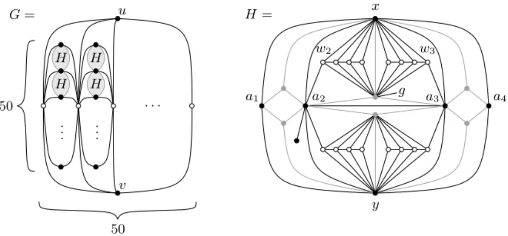
Proposition 1. There is a planar graph G with tw(G) = 3 and b(G) = 3. The graph G is depicted in the left of Fig. 4 and it is constructed in the following way: Two vertices u and v together with 50 white vertices form an induced K2,50
subgraph, i.e., a complete bipartite graph on 2 + 50 vertices. Any two consecu-tive white vertices together with 50 black vertices form another induced K2,50.
Finally, between any two consecutive black vertices the graph H is suspended, which is the 29-vertex graph depicted in the right of Fig. 4. This graph is clearly planar. Furthermore one can find a planar 3-tree containing G, i.e., G is planar and has treewidth at most 3.
G= H= H H H H x y u v 50 50 .. . ... · · · a1 a2 a3 a4 g w2 w3
Fig. 4. A planar graph G with tw(G) = 3 and b(G) = 3.
Proof. It is known [1] that b(K2,n) = 2 if n ≥ 5. Hence b(G) ≥ 2. For the sake
of contradiction let us assume that b(G) = 2 and consider a 2-bend representa-tion of G together with the induced 2-bend representarepresenta-tions of all induced K2,50
subgraphs. Furthermore, it is known [2] that in any EPG representation of K2,n
at most 12 vertices of the n-bipartition class represent their two edges using the same or consecutive segments. Moreover the 2-bend paths of u and v together have at most 12 endpoints of segments. Thus at most another 12 white vertices contain an endpoint of u or v in the interior of a segment. Hence there are two consecutive white vertices, say u0 and v0, that establish their edges with u and
v with two distinct segments of the same direction, say vertically. Both these segments are completely contained in the corresponding segment of u and v. Now the same argument can be applied to the K2,50subgraph induced by u0, v0,
and 50 black vertices. Thus there are two consecutive black vertices, which we denote by x and y, that establish their two edges with u0and v0with two distinct
segments of the same direction, each completely contained in the corresponding segment of u0and v0. Moreover, x and y intersect u0and v0 on the same segment
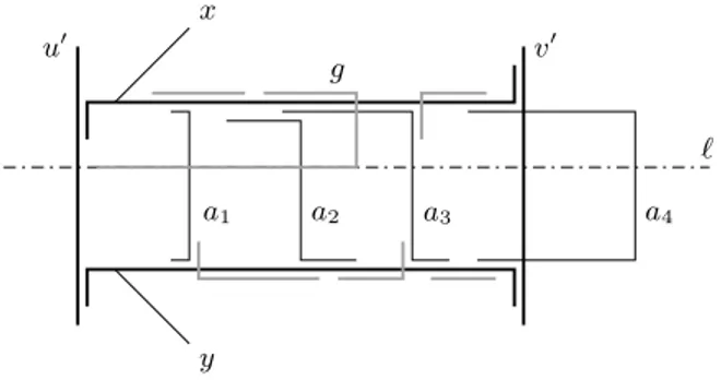
of u0 and v0, respectively. We conclude that the paths of u0, v0, x, and y are
positioned as the black bold paths in Fig. 5.
u0 v0 x y g a1 a2 a3 a4 `
Fig. 5. A detail of a hypothetical 2-bend representation of G.
Now consider the subgraph H which is suspended between x and y. W.l.o.g. we assume that the segments which display x and y are horizontal. The graph H contains, aside from x and y, a set A of four black vertices denoted by a1, a2,
a3, and a4, and a set B of six gray vertices, see the right of Fig. 4. Every vertex
in A ∪ B is adjacent to x or y, but neither to u0 nor to v0. Hence each edge
of such a vertex with x or y is established horizontally. From the adjacencies between vertices in A ∪ B it follows that the vertical segments of a1, a2, a3, and
a4 appear in order – w.l.o.g. from left to right. Moreover the edge {a2, a3} is
not established vertically since a2 has a private neighbor. W.l.o.g. assume that
{a2, a3} is established within the x-segment, see Fig. 5. Let us denote the gray
It follows that the horizontal segment of g within the x-segment is completely covered by a2and a3and hence lies strictly between a1 and a4. In consequence,
the six white vertices that are adjacent to x and g, but not to a2 or a3, intersect
gon its second horizontal segment. Let us denote the set of eight white vertices, which are common neighbors of g and x by W and the horizontal line supporting at least six edges between g and W by `. Evidently, the segment of g on ` crosses only one of {a1, a4}, but not both, say it does not cross a4, see Fig. 5.
The vertex in W that is adjacent to a2, respectively a3, is denoted by w2,
re-spectively w3. One can check that for i = 1, 2 the edge between wiand its white
neighbor is established on ` and moreover that w2 lies to the left of w3 on `.
This implies that the white vertices inside the triangle {x, g, w3} intersect the
horizontal x-segment to the right of a4. In order to establish their adjacency
with g all these three paths contain the part of ` between a3 and a4, making
them pairwise adjacent, which in G they are not – a contradiction. ut
4
4-bend representation for planar graphs
We show that the bend-number of every planar graph is at most 4, improving the recent upper bound of 5 due to Biedl and Stern [2]. Our proof is constructive and can indeed be seen as a linear-time algorithm to find a 4-bend representation of any given planar graph. We use the folklore fact that every plane triangu-lation can be constructed from a triangle by successively glueing 4-connected triangulations into inner faces. In every step our algorithm constructs a 4-bend representation Γ0 of a 4-connected triangulation G0 and incorporates it into
the already defined representation. The construction of Γ0 is based on a
well-known representation of subgraphs of 4-connected triangulations by touching axis-aligned rectangles. These are the basic steps of the algorithm:
1.) Fix some plane embedding of the given planar graph and add one vertex into each face to obtain a super-graph G that is a triangulation. If we find a 4-bend representation for G, removing the paths from it that correspond to added vertices, results in a 4-bend representation of the original graph. 2.) Construct a 4-bend representation of the outer triangle of G so that invariant
I, presented ahead, is satisfied.
3.) Let Γ0and G0 denote the so far defined 4-bend representation and the graph
that is represented, respectively. The graph G0 will always be a plane
trian-gulation, which is an induced subgraph of G. We repeat the following two steps 4.) and 5.) until we end up with a 4-bend representation Γ of the entire triangulation G.
4.) Consider a triangle ∆ which is an inner face of G0, but not of G. Let G ∆ be
the unique 4-connected triangulated subgraph of G, which contains ∆ and at least one vertex lying inside of it. (No vertex in G∆, except those in ∆,
is represented in Γ0.)
5.) Construct a 4-bend path for every vertex in G∆\∆ and add it to the
rep-resentation Γ0 so that all edges of G
4-bend representation of G0∪ G
∆. Additionally, we ensure that our invariant
is satisfied for every inner facial triangle of G0∪ G ∆.
The algorithm described above computes a 4-bend representation for every given planar graph. Moreover, steps 1.) to 3.) can easily be executed in linear time. For an efficient implementation of step 4.) we first identify all separating triangles of G, which can be in linear time [14]. The graph G∆ then arises from G by
removing all vertices in the exterior of the triangle ∆ and all vertices in the interior of every remaining separating triangle different from ∆. This can for example be done in O(|V (G∆)|) if G is stored with adjacency lists.
The crucial part is step 5.), i.e., the construction of a 4-bend representation of the 4-connected triangulation G∆. Our construction relies on a well-known geometric
representation of proper subgraphs of 4-connected plane triangulations. Actually, we need the slight strengthening in Lemma 1 below. A plane non-separating near-triangulation, NST for short, is a plane graph on at least four vertices without separating triangles such that all inner faces are triangles and the outer face is a quadrangle. For example, if G is a plane 4-connected triangulation and e = (u, w) an outer edge of G, then G\(u, w) is an NST.
Lemma 1. Let G = (V, E) be an NST. Then G can be represented as follows: (a) There is an axis-aligned rectangle R(v) for every v ∈ V .
(b) Any two rectangles are either disjoint or intersect on a line segment of non-zero length.
(c) The rectangles R(v) and R(w) have a non-empty intersection if and only if (v, w) is an edge in G.
Additionally, for every v ∈ V there is a vertical segment tv from the bottom to
the top side of R(v), such that the following holds:
(d) The segment tv lies to the right of tw for every v ∈ V and R(w) touching
the top side of R(v).
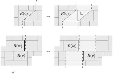
Proof. It is well-known that every NST has a representation with touching rect-angles, i.e., items (a)–(c) hold [16, 17, 20]. Moreover, those rectangles can be computed in linear time. We take such a rectangle representation and apply two modifications to it as illustrated in the top and bottom of Fig. 6, respectively. The modifications operate on the incidence relation of segments in the repre-sentation, that is, the inclusion-maximal horizontal and vertical lines. However, what follows is a more easily interpreted graphic image of the situation. For the first modification we define for every inner rectangle R(v) a line `, like the dashed one in Fig. 6. To be precise, ` consists of two vertical rays, one starting at the contact between R(v) and the leftmost rectangle touching the bottom side of R(v), and one starting at the contact between R(v) and the rightmost rectangle touching the top side of R(v). Those vertical rays are connected inside R(v), e.g., by a straight line segment. Then the plane is cut along ` and pulled apart to the left and right while extending every rectangle that has been cut by
`. As soon as the lower ray in the right part lies to the right of the upper ray in the left part we define the segment tv to lie between those two rays.
Having applied this modification to every inner rectangle, each segment tv is
spanned between the rightmost rectangle touching the top of R(v) and the left-most rectangle touching the bottom of R(v), for every v ∈ V .
R(v) R(v) R(v) R(v) R(w) R(w) tv ` `0
Fig. 6. Top: The modification at an inner rectangle and the positioning of the segment tv. Bottom: The modification at a pair R(v), R(w), with R(w) being the rightmost
rectangle touching the top of R(v).
For the second transformation another line `0 is defined for every pair of a
rect-angle R(v) and its rightmost rectrect-angle R(w) touching the top side of R(v). Again `0 contains two rays which both start in R(v) ∩ R(w). The ray emerging
down-wards starts to the left of tv and the ray going upwards starts to the right of tw.
Both rays are connected by a straight line segment contained in R(v) ∩ R(w). Similarly to the first modification, the plane is cut along `0 and pulled apart
(extending every rectangle that is cut by `0) until t
wlies to the left of tv.
Having applied this second modification to every pair of a rectangle R(v) and its right-most top neighbor R(w), condition (d) in Lemma 1 is fulfilled. Moreover, operating on the combinatorics of segments only, each modification can be done in constant time. Hence we obtain a linear-time algorithm, which completes the
proof. ut
Remark 1. There is an alternative proof of Lemma 1 that, however, involves some concepts. It is known that rectangle representations are in bijection with so-called transversal structures [7]. Given a transversal structure, one can split a vertex v into two adjacent vertices v0 and v00, distribute the neighbors of v
among v0 and v00 to have a triangulation again, and carry over the transversal
rectangle representation corresponding to the new transversal structure the right side of R(v0) coincides with the left side of R(v00). In other words, R(v0) ∪ R(v00)
is a rectangle with a vertical segment tv. This attempt directly gives a
linear-time algorithm to compute a rectangle representation satisfying items (a)–(d) in Lemma 1.
We will refer to a set of rectangles satisfying (a)–(d) in Lemma 1 as a rectangle representation of G. Rectangle representations are also known as rectangular duals. It is easily seen that every inner (triangular) face ∆ = {u, v, w} of G corresponds to a unique point in the plane given by R(u) ∩ R(v) ∩ R(w), i.e., the common intersection of the three corresponding rectangles.
Now we describe our invariant mentioned in steps 2.) and 5.) above.
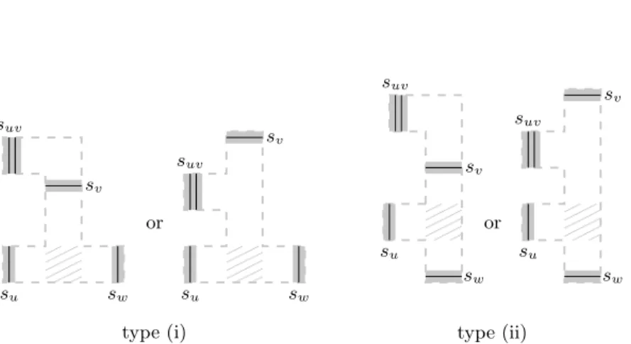
Invariant I: Let G0 be a plane triangulation. A 4-bend representation Γ0 of G0
is said to satisfy invariant I if there are mutually disjoint regions, i.e., polygonal parts of the plane, associated with the inner facial triangles of G0. For each inner
facial triangle ∆ = {u, v, w} we require that inside the region for ∆ there are segments su, sv, sw, and suv displaying u, v, w, and the edge {u, v}, respectively,
such that (up to grid-symmetry) each of the following holds.
(a) Segment su is vertical, sv is horizontal, lying to the top-right of su.
(b) Segment suv lies above su on the same grid line.
(c) Segment swlies to the right of suand not to the left of sv, and is of
one of the following types
(i) swis vertical and sees su.
(ii) swis horizontal and sees sv.
00 00 00 00 11 11 11 11 00 00 00 00 11 11 11 11 0000 00 00 11 11 11 11 00 00 00 00 11 11 11 11
type (i) type (ii) su su su su sv sv sv sv sw sw sw sw or or suv suv suv suv
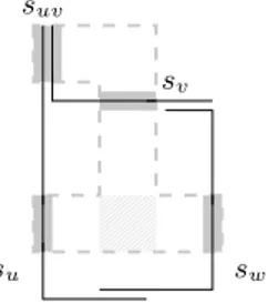
Fig. 7. The regions of type (i) and type (ii) for a triangle ∆ = {u, v, w} (up to grid-symmetry). The part of the region that can be seen by each of su, sv, and sw is
See Fig. 7 for an illustration. The regions are illustrated by the dashed line in Fig. 7. It is important that the regions in Fig. 7 may appear reflected and/or rotated by 90 degree.
Our algorithm to find a 4-bend representation of a planar graph executes steps 1.) to 5.) as described above. It is not difficult to find a 4-bend representation Γ0 of a triangle in step 2.) which satisfies invariant I, see Fig. 8.
su
sv
sw
suv
Fig. 8. An EPG representation of a triangle ∆ = {u, v, w} satisfying invariant I of type (i).
Hence we only have to take care of step 5.), which boils down to the following. Lemma 2. Let {P (u), P (v), P (w)} be a 4-bend representation of a triangle ∆ = {u, v, w} which satisfies invariant I, and G be a 4-connected triangulation whose outer triangle is ∆. Then {P (u), P (v), P (w)} can be extended to a 4-bend rep-resentation Γ of G which satisfies invariant I, such that every new 4-bend path, as well as the region for every inner face of G, lies inside the region for ∆. Moreover, such a representation can be found in linear time.
Proof. For convenience we rotate and/or flip the entire representation such that the region for ∆ is similar to one of Fig. 7, i.e., su and suv are the leftmost
segments and suv lies above su. Define G0= G \ {u, w} if the region for ∆ is of
type (i), and G0 = G \ {v, w} if the region for ∆ is of type (ii). By Lemma 1
G0 can be represented by rectangles so that conditions (a)–(d) are met. We put
this rectangle representation into the part of the region for ∆ which can be seen by each of su, sv, and sw. This part is highlighted in Fig. 7.
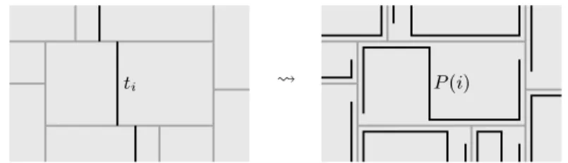
Now we explain how to replace the rectangle by a path for every vertex i 6= u, v, w in G0. We start with a snake-like 4-bend path P (i) within the rectangle
corresponding to i. To be precise, P (i) starts at the bottom-left corner of R(i), goes up to the top-left corner, where it bends and goes right up to the segment ti, which is defined in Lemma 1. Then P (i) follows along ti down to the bottom
side of R(i), where it bends and goes to the right up to the bottom-right corner and then up to the top-right corner. Afterwards, every path P (i) is shortened at both ends by some amount small enough that no edge-intersection is lost. See Fig. 9 for an illustration. Note that if R(j) touches the top side of R(i), then the
paths P (i) and P (j) do have an edge-intersection because ti lies to the right of
tj.
ti P(i)
Fig. 9. The 4-bend snake-like path P (i) within the rectangle R(i) corresponding to i.
It is not difficult to see, that these snake-like paths form a 4-bend representation of G0\{u, v, w}. The remaining edges in G0, i.e., those incident to u, v or w, are
established by extending the paths corresponding to the neighbors of u, v and w in G0. What follows is illustrated with an example in Fig. 10. Let x be the
unique4 neighbor of u and v in G. For every neighbor i 6= x of v the upper
horizontal segment of P (i) is shifted up onto the segment sv (extending the left
and the middle vertical segment of P (i)). Similarly, for every neighbor i 6= x of u the leftmost vertical segment of P (i) is shifted to the left onto the segment su (extending the upper horizontal segment of P (i)). For the case i = x, the
upper horizontal segment of P (x) is shifted up onto some horizontal line through suv. Then the leftmost vertical segment of P (x) is shifted to the left onto the
segment suv, and shortened such that it is completely contained in suv. The
paths of neighbors of w are extended according to the type of the region for ∆. If the region is of type (i), the rightmost vertical segment of P (i) for every neighbor i of w is shifted to the right onto sw. If the region is of type (ii), the
lower horizontal segment of P (i) is shifted down onto sw. Let us again refer to
Fig. 10 for an illustration.
Including the already given paths P (u), P (v), and P (w) gives a 4-bend repre-sentation Γ of G. It is easy to see that Γ is indeed representing the graph G and that the above construction can be done in linear time.
It remains to show that Γ satisfies invariant I. We have to identify a region for every inner facial triangle of G, such that each region lies within the region for ∆and all regions are pairwise disjoint. Therefore let ∆0= {u0, v0, w0} be such an
inner facial triangle. First, assume that none of {u0, v0, w0} is a vertex of ∆. This
is, ∆0 consists of inner vertices only. Then the intersection R(u0) ∩ R(v0) ∩ R(w0)
of the corresponding rectangles is a single point in the region for ∆. Moreover, exactly one of the three rectangles has its bottom-left or top-right corner at this point. Hence, the paths P (u0), P (v0) and P (w0) locally look like in one of the
cases in Fig. 11. In the figure, for each case a region for ∆0 = {u0, v0, w0} is
highlighted. Note that these regions can be chosen to be pairwise disjoint.
4
su su sv sv sw sw P(x) P(x) P(y) P(y) P(z) P(z) suv suv
type (i) type (ii)
Fig. 10. Examples of the 4-bend representation Γ contained in the region for ∆. The new regions of the three facial triangles that contain two vertices from ∆ are high-lighted. P(u0) P(u0) P(u0) P(u0) P(v0) P(v0) P(v0) P(v0) P(w0) P(w0) P(w0) P(w0)
Fig. 11. The four possibilities for an inner face ∆0= {u0, v0, w0} of G with at most one
vertex from ∆. The region for ∆0 is highlighted.
Similarly, if exactly one of {u, v, w} is a vertex in ∆0, then there is a point on the
corresponding segment (su, sv or sw) where the paths P (u0), P (v0) and P (w0)
locally look like in the previous case. Hence in this case we find a region for ∆0,
too.
Finally, exactly three inner facial triangles in G contain exactly two outer ver-tices. The regions for these three faces are defined as highlighted in Fig. 10. More formally, the region for the triangle {u, v, x} contains the segments s0
u, s0v, s0x,
and s0
uv which are contained in su, sv, the middle vertical segment of P (x), and
suv, respectively. The region for the triangle {u, w, y} contains the segments s0u,
s0
w, s0y, and s0wy, which are contained in su, sw, the lower horizontal (type (i))
or the middle vertical (type (ii)) segment of P (y), and P (y) ∩ sw, respectively.
Finally, the region for the triangle {v, w, z} contains the segments s0
and s0
wz, which are contained in sv, sw, the lower horizontal (type (i)) or the
rightmost vertical (type (ii)) segment of P (z), and P (z) ∩ sw, respectively.
All these regions are pairwise disjoint and completely contained in the region for ∆. We remark that even in case5x= y = z the above definitions of 4-bend paths and regions meet the required properties, see Fig. 12.
su su sv sv sw sw suv suv P(x) P(x)
type (i) type (ii)
Fig. 12. The case x = y = z for a type (i) region and a type (ii) region in the proof of Lemma 2.
Since G does not contain separating triangles, x, y, and z either all coincide or are pairwise distinct, which completes the proof of the lemma. ut Lemma 2 gives a construction as required in step 5.) of our algorithm. Hence, we have proved our main theorem.
Theorem 3. The bend-number of a planar graph is at most 4. Moreover, a 4-bend representation can be found in linear time.
Putting Theorem 3 and Proposition 1 together we have shown the following. Theorem 4. In an EPG representation of a planar graph 4-bend paths are al-ways sufficient and 3-bend paths are sometimes necessary, i.e., the maximum bend-number among all planar graphs is 3 or 4.
5
Conclusions
Although we could raise the previously known lower and upper bound, it remains open to determine the maximum bend-number of planar graphs.
5
Conjecture 1. There is a planar graph G, such that every EPG representation of G contains at least one path with four bends.
Another interesting class of representations is as edge-intersection graphs of ar-bitrary polygonal paths. It is straight-forward to obtain a 4-bend representation from a representation of touching >s and ⊥s [5]. What is the right answer?
References
1. Andrei Asinowski and Andrew Suk, Edge intersection graphs of systems of paths on a grid with a bounded number of bends, Discrete Appl. Math. 157 (2009), no. 14, 3174–3180.
2. Therese Biedl and Michal Stern, On edge-intersection graphs of k-bend paths in grids, Discrete Math. Theor. Comput. Sci. 12 (2010), no. 1, 1–12.
3. Hans L. Bodlaender, A partial k-arboretum of graphs with bounded treewidth, The-oret. Comput. Sci. 209 (1998), no. 1-2, 1–45.
4. Martin L. Brady and Majid Sarrafzadeh, Stretching a knock-knee layout for mul-tilayer wiring, IEEE Trans. Comput. 39 (1990), no. 1, 148–151.
5. Hubert de Fraysseix, Patrice Ossona de Mendez, and Pierre Rosenstiehl, On tri-angle contact graphs, Combin. Probab. Comput. 3 (1994), no. 2, 233–246. 6. Ehab S. El-Mallah and Charles J. Colbourn, On two dual classes of planar graphs,
Discrete Math. 80 (1990), no. 1, 21–40.
7. ´Eric Fusy, Combinatoire des cartes planaires et applications algorithmiques, PhD Thesis, 2007.
8. Martin C. Golumbic, Marina Lipshteyn, and Michal Stern, Representing edge in-tersection graphs of paths on degree 4 trees, Discrete Math. 308 (2008), no. 8, 1381–1387.
9. , Edge intersection graphs of single bend paths on a grid, Networks 54 (2009), no. 3, 130–138.
10. Daniel Gon¸calves and Pascal Ochem, On some arboricities in planar graphs, Elec-tronic Notes in Discrete Mathematics 22 (2005), 427 – 432, 7th International Col-loquium on Graph Theory.
11. Andr´as Gy´arf´as and Douglas West, Multitrack interval graphs, Proceedings of the Twenty-sixth Southeastern International Conference on Combinatorics, Graph Theory and Computing (Boca Raton, FL, 1995), vol. 109, 1995, pp. 109–116. 12. Frank Harary and William T. Trotter, Jr., On double and multiple interval graphs,
J. Graph Theory 3 (1979), no. 3, 205–211.
13. Daniel Heldt, Kolja Knauer, and Torsten Ueckerdt, Edge-intersection graphs of grid paths – the bend-number, preprint, arXiv:1009.2861v1 [math.CO], 2010. 14. Alon Itai and Michael Rodeh, Finding a minimum circuit in a graph, SIAM Journal
on Computing 7 (1978), no. 4, 413–423.
15. Alexandr V. Kostochka and Douglas B. West, Every outerplanar graph is the union of two interval graphs, Proceedings of the Thirtieth Southeastern International Conference on Combinatorics, Graph Theory, and Computing (Boca Raton, FL, 1999), vol. 139, 1999, pp. 5–8.
16. Krzysztof Ko´zmi´nski and Edwin Kinnen, Rectangular dual of planar graphs, Net-works 15 (1985), no. 2, 145–157.
17. Yen-Tai Lai and Sany M. Leinwand, An algorithm for building rectangular floor-plans, 21st Design Automation Conference (DAC ’84), 1984, pp. 663–664.
18. Bernard Ries, Some properties of edge intersection graphs of single bend path on a grid, Electronic Notes in Discrete Mathematics 34 (2009), 29 – 33, European Conference on Combinatorics, Graph Theory and Applications (EuroComb 2009). 19. Edward R. Scheinerman and Douglas B. West, The interval number of a planar graph: three intervals suffice, J. Combin. Theory Ser. B 35 (1983), no. 3, 224–239. 20. Peter Ungar, On diagrams representing maps, Journal of the London Mathematical