HAL Id: tel-01753184
https://tel.archives-ouvertes.fr/tel-01753184
Submitted on 29 Mar 2018HAL is a multi-disciplinary open access archive for the deposit and dissemination of sci-entific research documents, whether they are pub-lished or not. The documents may come from teaching and research institutions in France or abroad, or from public or private research centers.
L’archive ouverte pluridisciplinaire HAL, est destinée au dépôt et à la diffusion de documents scientifiques de niveau recherche, publiés ou non, émanant des établissements d’enseignement et de recherche français ou étrangers, des laboratoires publics ou privés.
variétales et exploitation des ressources génétiques des
plantes pour contrôler cette adaptation
Lucie Tamisier
To cite this version:
Lucie Tamisier. Adaptation des populations virales aux résistances variétales et exploitation des ressources génétiques des plantes pour contrôler cette adaptation. Sciences agricoles. Université d’Avignon, 2017. Français. <NNT : 2017AVIG0696>. <tel-01753184>
Université d’Avignon et des Pays de Vaucluse
Ecole doctorale 536 « Agrosciences et Sciences »
THESE
Pour obtenir le grade de
DOCTEUR DE L'UNIVERSITE D’AVIGNON ET DES PAYS DE VAUCLUSE
présentée et soutenue publiquement par
Lucie TAMISIER
le 7 décembre 2017
Adaptation des populations virales aux résistances
variétales et exploitation des ressources génétiques
des plantes pour contrôler cette adaptation
Thèse dirigée par Benoît MOURY et Alain PALLOIX
Jury :
Bruno Le Cam, Directeur de Recherche, INRA
Olivier Le Gall, Directeur de Recherche, INRA
Laurence Albar, Chargée de Recherche, IRD
François Delmotte, Directeur de Recherche, INRA
Julie Lederer, Chargée de Recherche, HM Clause
Benoît Moury, Directeur de Recherche, INRA
Rapporteur
Rapporteur
Examinatrice
Examinateur
Examinatrice
Directeur de thèse
1
Remerciements
Ce travail de thèse a été réalisé au sein des unités de recherche de Génétique et Amélioration des Fruits et Légumes (GAFL) et de Pathologie Végétale (PV) de l’INRA d’Avignon avec le soutien de la région PACA, du département BAP ainsi que du métaprogramme SMaCH. Cette thèse a également été soutenue par la société HM Clause à qui j’adresse mes remerciements.
Je tiens tout d’abord à remercier les membres de mon jury de thèse d’avoir accepté d’évaluer mon travail : merci à Bruno Le Cam et Olivier Le Gall pour leur travail de rapporteur. Merci également à Laurence Albar, François Delmotte et Julie Lederer d’avoir accepté d’être les examinateurs de ma thèse.
Je souhaite également remercier les membres de mon comité de thèse pour leurs remarques et leurs suggestions constructives concernant mes travaux de recherche. Merci à Charles-Eric Durel, Frédéric Fabre, FabienHalkett, Julie Lederer et Christopher Sauvage.
Mes premières pensées en écrivant ces remerciements s’adressent naturellement à Alain. Je garde de lui le souvenir d’un directeur particulièrement bienveillant et sympathique, passionné par son métier et qui savait transmettre son savoir avec enthousiasme et talent. Il aura accompagné et inspiré de nombreux jeunes chercheurs, et je sais que c’est une chance pour moi d’en avoir fait partie.
Je tiens ensuite à adresser un immense merci à Benoît. Travailler avec quelqu’un d’aussi passionnant, enthousiaste et investi a été un réel plaisir et a grandement contribué à rendre mon expérience de thèse positive et formatrice. Merci d’avoir été un directeur toujours disponible, que ce soit pour les discussions scientifiques, la participation aux manips ou les corrections de la thèse. J’ai pu bénéficier grâce à toi d’un encadrement extrêmement enrichissant et je t’en remercie sincèrement.
Je remercie également l’ensemble des techniciens avec qui j’ai eu l’occasion de travailler durant ces trois années. Marion et Ghislaine, un immense merci de m’avoir toujours soutenue dans mes grosses manips en faisant preuve d’une organisation sans faille. Cette thèse n’aurait pas pu se faire sans votre aide et je sais que j’ai eu beaucoup de chance de travailler avec des
2
le meilleur et j’espère que tu t’épanouiras dans tes nouveaux projets.
Merci également à Grégory pour toute l’aide que tu m’as apportée, notamment en début de thèse pendant les semaines d’extraction, ainsi qu’à Pauline et à Karine pour votre implication face aux montagnes de plaques ELISA. Je tiens également à remercier Nathalie, Joël et l’ensemble des équipes techniques qui s’occupent si bien des plantes. Merci aussi à Catherine et ses étiquettes qui m’ont été d’une aide précieuse pour organiser au mieux mes expériences, ainsi qu’à Patrick pour l’aide en ELISA et les conseils pour les photos.
Le génotypage des piments aura été un travail de longue haleine qui s’est bien déroulé grâce à plusieurs collègues qui m’ont permis de bénéficier de leur expertise. J’adresse donc de très grands remerciements à Renaud pour nous avoir si bien formées Marion et moi à l’extraction d’ADN, à Sylvain pour ses conseils avisés sur le GBS et le travail réalisé par son équipe sur les banques et enfin à Gautier pour m’avoir accueillie à Montpellier et pour l’aide qu’il m’a apportée sur le traitement des données.
Le séquençage des populations virales a également été le fruit d’un travail collaboratif. Merci à Catherine pour m’avoir accueillie à Toulouse et permis de participer au séquençage de mes échantillons. Un grand merci également à Frédéric et Elsa pour leur super modèle qui m’a fourni des données essentielles.
Je tiens aussi à remercier tous les membres des équipes Résistance Durable chez les Solanacées (RDS) et Virologie que j’ai côtoyés durant ma thèse. Un merci particulier à Karine et Emmanuel pour les discussions scientifiques (et les repas !) ainsi qu’à Judith pour nos échanges et son aide lors des dernières expériences. Merci aussi à nos supers secrétaires Claudine et Pascale pour tous les aspects administratifs.
J’ai également une pensée pour tous les collègues qui ont rendu mon séjour au château agréable. Je remercie notamment Joël qui partageait le bureau d’à côté et bon nombre de mes pauses café. Merci pour ton humour, ta bonne humeur permanente, tes petits tours (au sens propre) dans mon bureau, mais aussi pour tous tes conseils. Je remercie également Jean-Paul pour la disponibilité et l’efficacité dont il a fait preuve lorsque j’avais besoin d’aide en bioinformatique.
3
Un grand merci à tous les doctorants et collègues que j’ai pu côtoyer en dehors, pour tous les à-côtés, les randonnées, les concerts, les jeudis « Explo » ou encore les soirées jeux qui me laissent d’excellents souvenirs de ce séjour avignonnais. Merci à Elise, Gaëtan, Stéphanie, Zoé, Anna, Benoît, Maxime, Carole ainsi qu’à tout le groupe des doctorants de Saint Paul. Un merci tout particulier aux membres des « ratatouilles », Mariem et Isidore, pour nos sessions guitare du jeudi que j’ai tant appréciées. Enfin, je remercie évidemment mes proches pour leur soutien, et notamment les amis de longue date. Elodie, c’est toujours un plaisir de partir à l’aventure avec toi. Marion, merci pour tous ces bons moments et vivement notre prochaine escapade musicale. Arno, mille mercis pour ta joie de vivre, pour nos débats interminables et surtout pour le soutien sans faille durant ces trois ans (Rise up!). Les parents, vous êtes les meilleurs, merci pour tout.
5
Liste des abréviations
ADN: Deoxyribonucleic acid ARN: Ribonucleic acid
AUDPC: Area under the disease progress curve bp: Base pair
CMV: Cucumber mosaic virus (genus Cucumovirus)
DAS-ELISA: Double antibody sandwich enzyme-linked immunosorbent assay DIECA: Diethyldithiocarbamate
DH: Doubled haploid dpi: Days post inoculation
ddRADseq: Double digest restriction-site associated DNA sequencing eIF(iso)4E: Eukaryotic initiation factor (iso)4E
eIF4E: Eukaryotic initiation factor 4E FDR: False discovery rate
GBS: Genotyping-by-sequencing GFP: Green fluorescent protein GLM: Generalized linear models
GWAS: Genome-wide association studies
h²: Heritability
LD: Linkage disequilibrium MOI: Multiplicity of infection MQM: Multiple QTL mapping
Ne: Effective population size
6
QTL: Quantitative trait locus RB: Resistance breaking
RT-PCR: Reverse-transcription polymerase chain reaction RdRp: RNA-dependent RNA polymerase
s: Selection coefficient
SNP: Single-nucleotide polymorphism TEV: Tobacco etch virus (genus Potyvirus)
ToMV: Tomato mosaic virus (genus Tobamovirus) VA: Viral accumulation
7
Sommaire
Remerciements Liste des abréviations Introduction générale
1 5 13
Introduction ... 17
A. Playing on genetic drift to improve plant disease control strategies ... 19
1 Using evolutionary principles to take control of plant pathogen adaptation ... 19
2 Why use genetic drift to increase the durability of crop resistance to disease? ... 23
3 Measures of genetic drift in pathogen populations at different stages of the plant infection process and at different scales ... 30
3.1 Empirical and modelling approaches to measure the effective population size of plant pathogen populations ... 30
3.2 Estimates of the effective population size of plant pathogens ... 33
3.2.1 Plant inoculation ... 34
3.2.2 Plant colonization ... 39
3.2.3 Plant-to-plant transmission ... 40
4 Agricultural practices to enhance the effect of genetic drift and decrease the evolutionary potential of pathogens ... 42
4.1 Decrease of the inoculum size and increase of the founder effect at within-host scale ... 42
4.2 Intra-host bottleneck and Muller’s ratchet ... 44
4.3 Superinfection exclusion ... 46
4.4 Reduction of pathogen dispersal and survival ... 47
5 Future issues ... 48 B. Le pathosystème piment-PVY ... 61 1 Le PVY ... 61 1.1 Description générale ... 61 1.2 Génome du PVY ... 61 1.3 Origine et classification ... 61 2 Le piment ... 63
2.1 Origine géographique et diversité ... 63
2.2 Génome du piment ... 64
2.3 Résistances aux potyvirus ... 66
8
2.3.2 Les résistances quantitatives ... 68
2.3.3 La combinaison gène majeur/QTL ... 69
3 Un modèle biologique pour l’étude de la durabilité des résistances ... 71
3.1 Mécanismes d’action des QTL pour orienter l’évolution des populations virales . 71 3.2 Mesure des forces évolutives imposées par la plante aux populations virales ... 76
C. Objectifs de la thèse ... 79
Chapitre 1 : Quantitative trait loci in pepper control the effective population size of two RNA viruses at inoculation ... 81
1 Introduction ... 83
2 Results ... 84
2.1 Very few primary infection foci are initiated by two PVY variants simultaneously ... 84
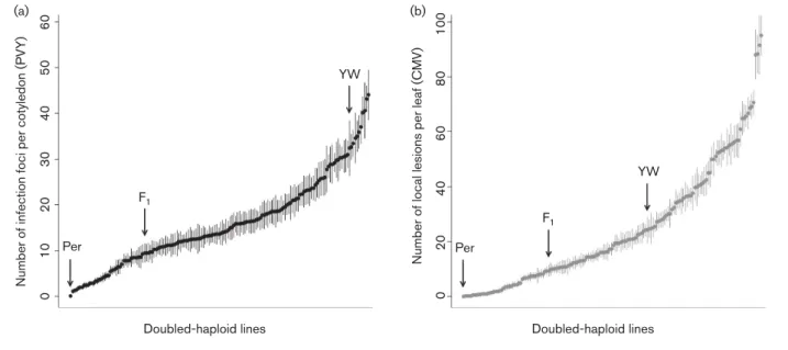
2.2 The numbers of primary infection foci and local lesions are highly heritable traits ... 84
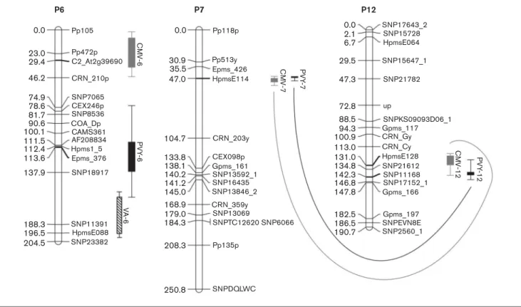
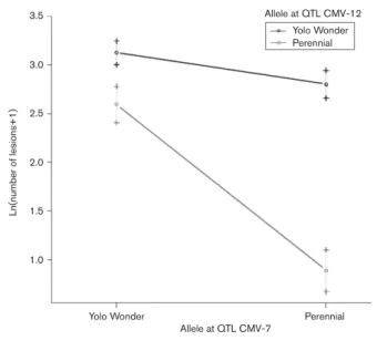
2.3 Detection of QTLs controlling the numbers of primary infection foci and local lesions for PVY and CMV ... 84
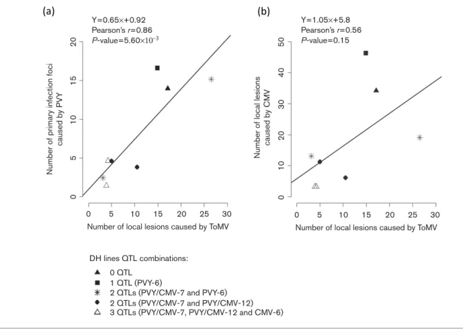
2.4 The number of infection foci induced by PVY correlates with the number of local lesions induced by ToMV ... 85
3 Discussion ... 85
3.1 Link between the number of primary infection foci or local lesions and the effective population size ... 85
3.2 Common and virus-specific QTLs control the effective population size of PVY and CMV at inoculation ... 87
3.3 Hypothesis on the mechanisms of action of the QTLs ... 88
3.4 Relationship between QTLs of effective population size and plant resistance ... 89
4 Methods ... 89
4.1 Plant and virus material ... 89
4.2 Evaluation of the Ne estimation method ... 90
4.3 Counting the primary infection foci and local lesion numbers induced by PVY, CMV and ToMV in a DH population ... 90
4.4 Statistical analyses ... 90
4.5 QTL analysis ... 90
9
Chapitre 2 : Genome-wide association mapping of QTLs implied in Potato virus Y
population sizes in the pepper germplasm ... 97
1 Introduction ... 100
2 Results ... 102
2.1 A core-collection representative of the pepper germplasm ... 102
2.2 Distribution of SNPs in the pepper genome ... 104
2.3 Population structure and kinship relationships ... 104
2.4 Variation in the number of primary infection foci and the virus accumulation among the pepper core-collection ... 107
2.5 Genome-wide association mapping of pepper resistance to PVY ... 108
3 Discussion ... 112
3.1 Benefits and limits of the pepper core-collection to perform genome-wide association ... 112
3.2 Common genetic factors control the effective population size at inoculation and the virus accumulation ... 114
4 Materials and methods ... 117
4.1 Pepper core-collection sampling ... 117
4.2 Phenotyping of the core-collection... 117
4.2.1 Number of PVY primary infection foci ... 117
4.2.2 Virus accumulation ... 117
4.3 SNP detection ... 118
4.4 Population structure and linkage disequilibrium estimations... 119
4.5 Genome-wide association study ... 119
4.6 Statistical analyses ... 120
5 Supplementary material ... 121
Chapitre 3 : Impact of genetic drift, selection and within-host accumulation on virus adaptation to its host plants ... 135
1 Introduction ... 138
2 Results ... 141
2.1 Estimates of Ne and s corresponding to a PVY composite population in 89 pepper DH lines ... 142
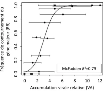
2.2 Correlation between putative explanatory variables and with the RB response variable ... 145
3 Discussion ... 150
10
3.2 Which evolutionary forces contribute most to resistance breaking? ... 151
3.3 Applied consequences to improve the durability of major-effect resistance genes ... 155
4 Materials and methods ... 156
4.1 Previous data ... 156
4.2 Analysis of composite PVY populations infecting pepper DH lines ... 157
4.3 Inference of virus Ne and s ... 159
4.4 Statistical analyses of the links between variables related to the evolution of PVY populations ... 159
5 Supplementary material ... 160
Chapitre 4 : Taking control of virus adaptation by choosing host plant genotype ... 167
1 Introduction ... 170
2 Results ... 173
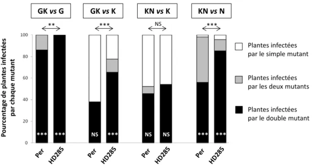
2.1 Divergent evolutionary trajectories among PVY lineages: extinction, status quo or parallel fixation of mutations ... 173
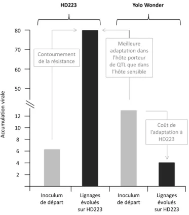
2.2 Significant increase in virus accumulation but little change in aggressiveness after experimental evolution ... 176
2.3 Validation of the impact of the two most frequent de novo mutations on virus accumulation ... 180
2.4 Contrasted effects of selection, genetic drift and initial accumulation on virus evolution ... 180
3 Discussion ... 183
3.1 Closely-related pepper lines impose divergent evolutionary trajectories to PVY ... 183
3.2 Choosing the plant traits most effective to avoid PVY adaptation ... 185
3.2.1 Relevance and precision of estimation of plant traits used to explain PVY evolutionary trajectories ... 185
3.2.2 Effects of plant traits on virus evolution ... 186
3.2.3 Agronomical perspectives ... 189
4 Materials and methods ... 190
4.1 Virus and plant material ... 190
4.2 Experimental evolution ... 191
4.3 Virus sequencing ... 192
4.4 Measures of aggressiveness and virus accumulation ... 192
4.5 Measures of virus competitiveness ... 193
11
5 Supplementary material ... 195
6 Complément d’information à l’article...201
Chapitre 5 : Discussion et perspectives ... 207
1 Synthèse des principaux résultats ... 208
2 Comparaison des approches employées ... 212
2.1 Cartographie de QTL en population biparentale et GWAS ... 212
2.2 Evolution expérimentale par passages successifs et mesure de la durabilité du gène majeur pvr23 ... 213
2.2.1 La méthodologie employée ... 213
2.2.2 Les résultats obtenus ... 217
3 Par quels mécanismes le fonds génétique contraint-il l’évolution des pathogènes ?.. 218
3.1 Effet des goulets d’étranglement sur les mutations adaptatives ... 218
3.2 Peut-on confirmer l’action du cliquet de Muller ? ... 220
4 Conséquences pour la sélection variétale et l’application en champs ... 221
5 Conclusion générale ... 225
Références bibliographiques Annexe
227 247
13
14
L'amélioration de la protection des cultures contre les agents pathogènes est un des enjeux majeurs de la recherche agronomique. Actuellement, le niveau global des pertes de production agricole engendrées par les agents pathogènes demeure élevé, des pertes allant de 26 à 40 % de la production en champs ayant été estimées selon les espèces (Oerke 2006). De plus, les risques d'émergence d'agents pathogènes sont accrus par les changements climatiques ainsi que l'augmentation des échanges commerciaux au niveau international qui favorisent l'introduction d'espèces dans de nouvelles zones géographiques (Anderson et al. 2004).
Afin de limiter les dégâts occasionnés par les bio-agresseurs, l'utilisation de pesticides a longtemps été la solution privilégiée. Cependant, l'impact néfaste de ces intrants sur la santé et l'environnement rend aujourd'hui nécessaire la mise en place de méthodes de lutte alternatives telle que la lutte génétique. Cette stratégie couramment employée consiste à sélectionner des variétés génétiquement résistantes vis-à-vis de l'agent pathogène ciblé. La principale limite de la lutte génétique est la capacité des agents pathogènes à s’adapter aux variétés résistantes. Plusieurs gènes majeurs sont ainsi devenus inefficaces après quelques années de culture seulement (McDonald and Linde 2002; García-Arenal and McDonald 2003). De plus, la sélection d'une nouvelle variété résistante n'est pas toujours possible car les gènes majeurs sont rares dans les collections variétales. Aussi, les pratiques de sélection des plantes, qui ont toujours privilégié l’efficacité de la protection, doivent maintenant prendre en compte sa durabilité afin de ne pas épuiser les ressources génétiques.
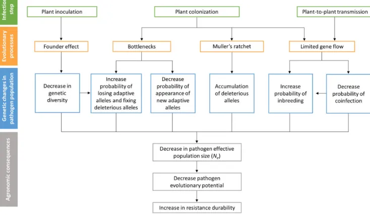
D’autres sources de résistances existent dans les ressources génétiques. Il s’agit des gènes de résistance quantitative ou QTL (Quantitative Trait Loci), qui ne font que réduire les dégâts dus aux épidémies mais qui sont beaucoup plus fréquents dans les collections variétales. Chez plusieurs pathosystèmes, la combinaison d’un gène majeur et de QTL dans une même variété a permis d’augmenter significativement la durabilité de la résistance (Palloix et al. 2009; Brun et al. 2010; Fournet et al. 2013). Les QTL ont ainsi empêché ou réduit le contournement du gène majeur en orientant l’évolution des agents pathogènes. On suppose que les QTL affecteraient l’évolution des populations de pathogènes en agissant sur différentes forces évolutives, notamment la dérive génétique et la sélection. L’association d’un gène majeur et de QTL est donc une stratégie prometteuse. En effet, l’enjeu de la durabilité deviendrait accessible en déployant des gènes de résistance en fonction non seulement de leur capacité à réduire les populations pathogènes mais aussi à orienter et contrôler leur évolution dans l’agrosystème.
15
Le sujet de cette thèse s’intègre donc dans le contexte de la durabilité des résistances variétales aux agents pathogènes et fait également appel à des concepts de biologie évolutive. Afin de comprendre au mieux les résultats présentés dans la suite de ce manuscrit, l’introduction se structurera en trois parties. Elle débutera par un article d’opinion portant sur l’intérêt d’utiliser la dérive génétique pour augmenter la durabilité des résistances aux pathogènes. Ensuite, le modèle d’étude piment (Capsicum annuum) – PVY (Potato virus Y) utilisé au cours de cette thèse sera présenté. Les résultats récemment obtenus sur la durabilité des résistances chez ce pathosystème y seront plus particulièrement développés. Enfin, les objectifs de la thèse seront énoncés.
17
19
A. Playing on genetic drift to improve plant disease control
strategies
Tamisier, L. (1,2), Fabre, F.(3), Papaïx, J. (4), Berthier, K. (2), Moury, B.(2).
(1) GAFL, INRA, 84140 Montfavet, France
(2) Pathologie Végétale, INRA, 84140 Montfavet, France
(3) UMR 1065 Santé et Agroécologie du Vignoble, INRA, Villenave d’Ornon, France (4) BioSP, INRA, 84000 Avignon, France
Keywords: genetic drift, evolutionary principles, plant disease management, effective population size
Abstract
The widespread use of monogenic resistances has proved to be an efficient method to fight against many plant diseases. However, the pathogen ability to evolve and breakdown these resistances is a major limit of this practice. Several authors have therefore highlighted the need to include evolutionary principles in the design of resistance management programs. They aim to limit pathogen evolutionary potential by playing on the evolutionary forces imposed by the pathogen environment. Among these forces, the role of selection to constrain pathogen evolution has been widely discussed. On the contrary, studies on the effects of genetic drift are scarce although it is one of the main evolutionary forces, even for plant microbe pathogens that possess huge census population sizes. In this opinion article, we argue that genetic drift should also be considered to achieve durable resistance. We discuss the benefits of genetic drift in the context of plant resistance durability, the different methods to assess its impact on pathogen population and we make proposals for its implementation in agricultural practices.
1 Using evolutionary principles to take control of plant pathogen
adaptation
In plants, major-effect resistance genes have been widely used to fight against pathogens and protect crops. These genes provide a high level of resistance against pathogens, are environmentally safe and relatively easy to use. However, the main drawback of this genetic
20
control is the ability of the pathogen to overcome the resistance gene. Indeed, the deployment of a resistance gene in the field will unavoidably exert a strong selective pressure on the pathogen population. Many pathogen microbes have high mutation rates, short generation times, huge census population sizes and they usually show high evolution rates. If a resistance-breaking pathogen variant appears by mutation, recombination or migration into the population, the strong selective pressure imposed by the major resistance gene will lead to a rapid increase of the variant frequency and eventually to its fixation in the population. As a consequence, the new pathogen population may be able to invade the population of hosts that carry the resistance gene and the resistance may become completely inefficient. A high number of examples of such resistance breakdowns exist in the literature (Parlevliet 2002). Alternative gene types or genetic constructions are therefore needed to achieve more durable resistances. Several authors have proposed to use population genetics principles to improve resistance breeding strategies (McDonald and Linde 2002; Kinkel et al. 2011; Thrall et al. 2011; Zhan et al. 2014; Brown 2015; Zhan et al. 2015). Their idea is to view the plant as an environment in which the pathogen population will evolve. In this respect, the evolutionary forces*1 that shape the pathogen population are therefore imposed by the plant itself. Indeed, the plant will select certain pathogen genotypes, will impose bottlenecks* to the pathogen population during the infection cycle, will impact the recombination rate between co-infecting pathogen variants by spatially structuring the population at the within-plant scale and will condition the fraction of possible mutations as well as their effects on pathogen fitness*. It is therefore of primary importance to understand how plant genotypes influence the evolution of pathogens during infection, because it could allow the breeding of plant cultivars preventing or limiting pathogen adaptation. Manipulating plant genetics according to selection* intensity (Brown 2015), mutation rate (Leach et al. 2001) and genetic drift* strength (Abel et al. 2015) to slow down pathogen adaptation has been discussed and experimented in several studies.
As mentioned above, plant resistance genes inherently exert selection effects on pathogen populations as far as there is some diversity in the capacity of infection of the resistance carrying plants among the pathogen population. Indeed, by definition, plant resistance reduces growth rate and potentially the within-host density of the pathogen. As soon as resistance-breaking (RB) variants, that escape the effect of the plant resistance gene, appear or are introduced into the pathogen population, differential selection effects are manifested in the resistance-carrying host plant. They can be defined as s = rRB – rWT, where rRB and rWT are the intrinsic growth rates
21
of the RB and wild-type (i.e. non-RB) pathogen variants. Multiple strategies have been proposed to use these differential selective effects to fight against crop pathogens. At the plant scale, the use of quantitative resistance* can slow down the evolution rate of the pathogens. This type of resistance confers only partial resistance and allows pathogens to accumulate in the plant and colonize it. Therefore, it decreases the competition among pathogen variants, making it a strategy potentially more durable than qualitative resistance conferred by a major gene, which, in contrast, can rapidly select and fix a RB allele in the pathogen population (Poland et al. 2009; Zhan et al. 2015). The slower action of selection on pathogens due to quantitative resistance has been observed for multiple pathosystems, such as Potato virus Y (PVY) with pepper (Quenouille et al. 2013) in the laboratory and in greenhouse as well as the barley pathogen Rhynchosporium secalis (Abang et al. 2006), and the wheat pathogens
Mycosphaerella graminicola (Zhan et al. 2002) and Phaeosphaeria nodorumin (Sommerhalder
et al. 2011) in the field. At the landscape scale, heterogeneity in the host population can impose divergent selective pressures on the pathogen population. The landscape can be represented as a heterogeneous environment with different fitness peaks. Pathogens will not be able to reach all adaptive peaks in this fitness landscape, which could increase the durability of the plant resistance genes used. Indeed, a pathogen variant able to infect multiple plant genotypes may have a lower infection efficiency than a pathogen specialized in one plant genotype of the mixture (Mundt 2002). This type of control is particularly efficient for diseases spread by spores, such as mildews and rusts. The efficiency of this strategy is more difficult to predict for pathogens like viruses, because the outcome also relies on the abundance and behavior of the vectors. Cultivar mixtures with different major resistance genes, different partial resistance genes or both can be used to impose this disruptive selection. This strategy has efficiently reduced the selection coefficient of P. nodorumin populations in the field. The genetic diversity of the pathogen population did not change during two years when evolving in a cultivar mixture of partially resistant hosts, whereas the pathogen evolution was faster in monoculture (Sommerhalder et al. 2011). Mixing resistant and susceptible cultivars has also been proposed to enhance resistance durability. One of the reasons is the dilution effect: non-RB pathogen variants will be maintained in the susceptible plant genotypes, whereas RB pathogen variants will probably be eliminated from these plants because of the fitness cost associated with the resistance breakdown. Using a mixture of susceptible and less-susceptible rice varieties to the blast disease in a large field scale, Zhu et al. (2000) have shown that the disease was reduced in both varieties and obtained 94% less severe rice blast than in monoculture. They explained it by the dilution effect of the inoculum of a strain thanks to the distance between the two varieties.
22
A significant decrease of Phytophthora infestans symptoms on potato was also obtained by mixing susceptible and resistant potato plants during two years (Garrett and Mundt 2000). Temporal patterning of the selective forces could also be applied using crop rotations. At the spatio-temporal scale, applying Red Queen* principles could help to limit the selection of pathogen variants (Zhan et al. 2015). The goal is to withdraw the crop carrying the resistance gene before the increase in frequency of the RB pathogen. The new crop will impose a negative selection on the variant, preventing its increase in the population.
Playing on the mutational trajectories accessible for the pathogen is another way to protect a major resistance gene from breakdown. Mutation can be used in two ways. First, the cost in fitness of a RB mutation can be too high for the mutation to be maintained in the population (Leach et al. 2001). In the absence of compensatory mutations, the RB strain will be removed from the population because of the action of negative selection. This is particularly true for pathogens with small genomes composed of multifunctional genes like viruses, where a small number of mutations can have strong negative impact on pathogen fitness (Carrasco et al. 2007). Indeed, plant durability is usually higher for plant resistance to viruses than to other plant pathogens because the genetic changes needed to overcome the resistance often imposed a very high fitness cost to the viruses (García-Arenal et al. 2003). The fitness cost associated to resistance-breakdown is the reason why, after a long period of deployment, some resistance genes are still effective against bacteria (Cruz et al. 2000) or viruses (Janzac et al. 2010). Second, the number of mutations needed to overcome the resistance is directly related to resistance durability (Harrison 2002). For viruses, if two or more mutations are needed to overcome the major gene, the resistance is usually considered as durable (Lecoq et al. 2004). The explanation for this outcome is that the intermediate variants, carrying one of the two mutations needed, are not necessarily fit enough to be maintained in the population and to acquire the second mutation. For example, in tobacco, the well-known N gene confers a highly durable resistance against Tobacco mosaic virus (TMV) because of the high number of mutations required to overcome the resistance (Padgett et al. 1997; Harrison 2002).
To date, the link between genetic drift and resistance durability has been less studied than for the other evolutionary forces, even is several authors have proposed to take advantage of this force to limit the emergence of adapted pathogens (Abel et al. 2015). We will see in the next section that genetic drift may, however, have a strong impact on resistance durability, and that this force should also be taken in consideration in plant disease control strategies.
23
2 Why use genetic drift to increase the durability of crop
resistance to disease?
Genetic drift is the random variation of allele frequencies from one generation to the next. Like selection, it always induces a loss of genetic diversity in the population over time. However, since genetic drift is a stochastic process, it leads to the fixation or the loss of alleles independently of their fitness effects. The population genetics parameter used to quantify the impact of genetic drift on the genetic structure of the population is the effective population size* (Ne). It is defined as the size of an ideal Wright-Fisher* population that would experience the
same amount of genetic drift as the population under study (Charlesworth 2009) (Box 1). When
Ne is small, the effect of genetic drift is strong and can overwhelm the action of selection, while
when Ne is high, the effect of genetic drift is low and selection is the predominant force. Wright
(1931) first introduced the concept of effective population size. He also demonstrated that, when population varies over time, Ne can be approximated as the harmonic mean of the effective
populations sizes over all generations. Since then, several methods have been developed to estimate Ne leading to the emergence of different concepts of Ne such as the variance effective
size, the inbreeding effective size, the eigenvalue effective size or the coalescent effective size (Ewens 1982; Crow and Denniston 1988; Caballero 1994; Nordborg and Krone 2002; Charlesworth et al. 2003; Wang 2005). For instance, the variance effective size measures the change in allele frequencies from generation to generation while the inbreeding effective size measures the rate of increase in homozygosity. These two measures are the most used, and in this article, we will essentially refer to the variance effective size. Another feature of Ne is that
it is usually much smaller than the census population size* (N). In the case of plant viruses for example, the size of a Tobacco mosaic virus (TMV) population infecting a tobacco leaf can reach between 1011 and 1012 viral particles (Gibbs et al. 2008), while Ne estimates range from
one to a few hundred particles (Zwart and Elena 2015). Since Ne is directly related to the amount
of genetic drift undergone by the population, it is more relevant to consider Ne than N when
24
Box 1. The joint effect of selection and genetic drift: illuminating example from
simulations of a Wright-Fisher model
The Wright-Fisher model occupies a central position in population genetics (Ewens 2004). It explicitly accounts for the effects of the main evolutionary forces – mutation, genetic drift and selection – on the dynamics of allele frequencies. The population considered in the Wright-Fisher model is an ideal population, which is a well-mixed, randomly-mating haploid population of finite size reproducing in discrete non-overlapping generations. The concept of ideal population is central for understanding the definition of effective population size, Ne.
Indeed, Ne is the size of an ideal population (i.e. obeying previous assumptions) that would
display the same degree of randomness in variant frequencies as the real population under study. Simulating allele frequencies over time with a Wright-Fisher model is a good way to visualize how genetic drift and selection impact evolution. Let’s consider a haploid population of constant size N with 2 alleles A and a and equal initial frequencies (p=q=0.5). In this situation,
N is equal to the effective population size (Ne). These 2 alleles can represent two virus variants
characterized by two alternative nucleotides at a given position in an RNA sequence. The allele
A has a selection coefficient s, its relative fitness being 1+s (the fitness of allele a is 1).
We simulated the dynamic of the frequencies of A using a Wright-Fisher model over an array of increasing N and s (Figure 1). Selection is a deterministic force that increases the frequency of the fittest variants at the expense of the weakest ones. Simulations highlighted that the distinctive footprint of selection is contained in the mean trajectories of variant frequency (Figure 1, compare each row). Genetic drift, unlike selection, acts equally on all variants. It is the outcome of random sampling effects between generations in finite population size (Charlesworth 2009). The distinctive footprint of genetic drift is contained in the variance of the trajectories of variant frequency, higher variance being associated to lower N (Figure 1, compare each column). These distinctive footprints can be used to jointly estimate selection and genetic drift by observing allele frequencies at several time points in independent hosts.
Classical results are illustrated throughout these simulations. First, with a neutral allele (Figure 1, a to c; first raw), the mean allele frequency remains constant: pA(t)= p. Half of A allele goes to fixation, half goes to extinction. This is a classical result: the proportion of populations expected to go to fixation for a given neutral allele is equal to its initial frequency (here 0.5).
25
The time to absorption (corresponding either to a loss or a fixation of A) increases with N as the effect of drift per generation becomes smaller. Allele A is always fixed or lost after 40 generations with N=10 (Figure 1a, d, g) whereas all the populations remained polymorph after 100 generations with the largest size considered (N=1000, Figure 1c). 5000 generations are then needed to go systematically to fixation or loss. In a haploid population, the mean time to fixation of a neutral allele depends on the population size and on its initial frequency. It is approximated by Tps(fix) = -(1/p)[2N(1-p)ln(1-p)] (Kimura and Ohta 1969). In figure 1 (a to c), the average times to fixation are 13.8 (N=10), 138 (N=100) and 1386 (N=1000) generations. Average times to fixation are quite fluctuating but are on the order of N (Rouzine et al., 2001). By contrast, average times to fixation are much less sensitive to the initial allele frequency (Figure 2a). When p is small, as for example in the case of a new variant generated by mutation, the average time to fixation of a neutral allele is 2N (Figure 2a, p=10-4). Indeed, for small p, ln(1-p)-p and the above formula provides Tps(fix) = 2N.
Figure 1: Simulations (20 replicates) of allele frequencies over 200 generations using bi-allelic Wright-Fisher model for 3 population sizes N (10, 100 and 1000) and 3 selection coefficients s (0, 0.01, 0.1). Initially the two alleles have equal frequencies. The mean trajectories correspond to the bold black lines. Probabilities of fixation (p(fix)) and extinction (p(extinct)) and the mean fixation time (Tps(fix)) are estimated after 5000 generations using 104 simulated trajectories.
(a) (b) (c)
(d) (e) (f)
26
Second, when selection and genetic drift act simultaneously, the dominant regime of evolution is controlled by the product Ns (Rouzine et al. 2001; Ewens 2004; Charlesworth 2009). If Ns<<1, then genetic drift predominates over selection and evolution is mostly stochastic (Figure 1, in particular panel (d) but also (e) and (f)). Allele dynamics behave close to neutrality. The fixation probability, close to initial allele frequencies, is almost independent of selection. So is the mean time to fixation. This is clearly illustrated in figure 2b (fixation probability) and in figure 2c (fixation time) for (s, N) pairs below the second diagonal (i.e.
Ns<1). The typical footprints of selection and genetic drift are then hard to distinguish, making
their joint inference a hard task. If Ns>>1, selection becomes effective and evolution is mostly deterministic (Figure 1, f, h, i). The beneficial allele considered almost always goes to fixation (Figure 2b for (s, N) pairs above the second diagonal (i.e. Ns>1)). The time to fixation is also considerably reduced compared to the neutral case (Figure 2c). The joint inference problem becomes much simpler in that case.
With both selection and drift, no analytical form of the mean time to fixation is available. Motoo Kimura derived an approximation of the probability of fixation of allele A as
(see Patwa and Wahl (2008) for a review).
Figure 2. (a): Expected time to fixation for a neutral allele as a function of effective population size for 3 initial frequencies. Lines converge to the dash line for which Tps(fix)=2N as initial frequency decreases. (b): Probability of fixation of a beneficial allele with selection coefficient s (x-axis) in an ideal bi-allelic Wright-Fisher population of size N (y-axis) and equal initial frequencies. (c): Same as B for the mean time to fixation when fixation occurred. Probabilities of fixation and mean fixation times are estimated after 5000 generations using 104 simulated trajectories. The gray dotted line (B and C)
separates the selection-drift space where sN<1 (below) and sN>1 (above).
(a) (b) (c)
1-exp(-2Nsp) 1-exp(-2Ns)
27
The main goal of this article is to highlight the important role of genetic drift imposed by the host on the pathogen populations and how we could use it to improve plant resistance durability. As we have seen above, a strong genetic drift will reduce the genetic variation of plant pathogen populations. Pathogen population with a high Ne (i.e. low genetic drift) have a
better ability to adapt and to potentially break down resistance genes or become resistant to antibiotics and fungicides. Consequently, we can hypothesize that a strong genetic drift will reduce the evolutionary potential* of the pathogen population and that it will avoid or slow down the adaptation of the population to the control method, leading to an increase in plant resistance durability. Both experimental studies and meta-analyses have provided evidences supporting these assumptions. Indeed, several experiments have demonstrated that the drastic reduction of population size through repetitive bottlenecks induced a strong genetic drift usually associated with a decrease of the pathogen’s fitness. These ‘mutation accumulation’ experiments consist in imposing repeatedly bottlenecks to the population through time. As a result, all mutations that are non-lethal can be randomly fixed independently of their fitness effects and without being eliminated by selection (Barrick and Lenski 2013). When these experiments are performed with asexual populations and in the absence of recombination events, a process called Muller’s ratchet* occurred (Box 2). It predicts that, since the majority of the mutations are deleterious, an irreversible accumulation of deleterious mutations will occur over time and will be responsible of a constant decrease in the mean fitness of the population. Eventually, the population may go to extinction because of a mutational meltdown (Lynch et al. 1993). The first experimental proof of this concept was provided by a famous experiment of Chao (1990). By passing the RNA bacteriophage Φ6 through a series of bottlenecks, he showed that the transferred clones had lost 78% of fitness compared to the parental clones. Since then, the Muller’s ratchet has also been proved to occur with animal RNA viruses such as the Vesicular stomatitis virus (Duarte et al. 1992) and the Foot-and-mouth disease virus (FMDV) (Escarmı́s et al. 1996). The action of Muller’s ratchet has also been demonstrated for the human immunodeficiency virus type 1 (HIV-1) (Yuste et al. 1999) and the herpes simplex virus type 1 (HSV-1) (Jaramillo et al. 2013). A loss in fitness through naturally occurring bottlenecks due to local lesions in plants has been shown for TEV (Tobacco
etch virus) as well (de la Iglesia and Elena 2007). The same results were obtained for bacteria
with Escherichia coli (Kibota and Lynch 1996) and for yeast with Saccharomyces cerevisiae (Zeyl and DeVisser 2001). Even if experiments directly testing the impact of bottlenecks on resistance durability are still needed, the multiple demonstrations that repetitive bottlenecks
28
caused a loss of evolutionary potential in the pathogen population are already a good indicator of the potential advantages of the use of genetic drift.
The problem of pathogens that evolve drug resistance in medicine field is a similar issue as plant resistance breakdown from an evolutionary viewpoint. Recently, Feder et al. (2016) have compared the HIV-1 sequences from patients treated with older drug therapies, where virus evolved rapidly and frequently acquired resistance, to HIV-1 sequences from patients treated with newer and more effective drugs, where the virus evolves slowly and rarely acquired resistance. They demonstrated that, when resistance mutation occurred, they were associated to an increase in genetic diversity with a less effective treatment and to a reduction in genetic diversity with an effective treatment. They propose that, in the case of old treatment administration, the same adaptive mutation can arise several times independently in different virus genetic backgrounds, leading to the higher genetic diversity observed, and can be predicted in a deterministic manner. In contrast, better drugs diminish the population size which decreases in turn the genetic diversity, the acquisition of drug resistance becoming partly an unlucky occurrence. These results suggest that a reduction in Ne and the increase in genetic drift
associated could be one of the mechanisms explaining the better efficacy of the new treatments. Meta-analyses on plant pathogens have also highlighted the fact that genetic drift could have a significant impact on resistance durability. Using data from 52 pathosystems, McDonald and Linde (2002) have developed a risk assessment model to estimate the risk of resistance breakdown according to the evolutionary potential of bacteria, fungi and nematodes. The evolutionary potential of the pathogens was determined by multiple criteria such as the mating system, the gene flow* intensity or the pathogen effective population size. In their model, the effective population size was a categorical variable with three levels: small, average and large. In this model, a small population size decreased the evolutionary potential of the pathogen. Even if it is an over simplification of the pathogens biology, they used it as a risk factor for crop damages and they concluded that disease management programs that maintain small pathogen population sizes are helpful to control resistance breakdown. García-Arenal and McDonald (2003) have performed the same analysis for plant viruses. They also showed that effective population size plays a role in the risk of resistance breakdown by viruses.
29
Box 2. Muller’s ratchet
This process describes the irreversible accumulation of deleterious mutations in an asexual population (Muller 1964). Every individual is sorted according to the number of deleterious mutations it carries. The class with the lowest number of deleterious mutations carries ‘n’ mutations, the class with one more deleterious mutation carries ‘n+1’ mutations etc. The appearance of a mutation will move an individual from one class to another. Selection will eliminated the classes carrying most of the deleterious mutations. Genetic drift will eliminate, by chance, the classes carried the lowest amount of mutations. In this model, there is no recombination allowed, as well as no reverse or compensatory mutations. Therefore, once eliminated by drift, the class with the lowest amount of mutations could not be recreated. Since there is no turning back, the number of deleterious mutations increases over time in a ratchet-like manner. Eventually, this irreversible accumulation of deleterious mutations can cause the extinction of the population. The speed of the ratchet is increased when the population size is small, the effect of genetic drift being stronger in small populations, when the mutation rate is high and when the negative selection against deleterious mutations is low (Gordo and Charlesworth 2000). The mechanism of Muller’s ratchet is not only useful to explain the extinction of asexual populations, but has also been used to explain the degeneration of Y chromosome, the evolution of sexual reproduction, the advantage of recombination and the limit to the genome size of asexual organisms (Charlesworth 1978; Engelstädter 2008).
Figure 3: Illustration of the Muller’s ratchet process. Each bar corresponds to a class of individuals carrying the same number of deleterious alleles. The effects of the evolutionary forces on the frequencies of these classes of individuals are drawn in red. Adapted from Lefevre et al. (2016).
30
All these results demonstrated that Ne is an important parameter to take into consideration
when studying pathogen adaptation to plant resistances. However, to take advantage of Ne, we
first need to accurately estimate it, with both empirical and mathematical approaches, and to understand its effects at different infection stages.
3 Measures of genetic drift in pathogen populations at different
stages of the plant infection process and at different scales
3.1 Empirical and modelling approaches to measure the effective population size
of plant pathogen populations
Two types of empirical approaches exist to measure Ne: direct and indirect methods. The
direct estimation method follows directly the demographic changes occurring in the population. For example, the size of a bottleneck is measured by quantifying the number of individuals that survive after the reduction of the population size. One way to measure the bottleneck size at inoculation for viruses is to use a host producing necrotic local lesions in response to the infection. In this case, the number of local lesions is a direct and easy estimation of the number of founders (Sacristán et al. 2011; Zwart and Elena 2015). This approach is not restricted to plants producing necrotic lesions. Using viruses expressing fluorescent markers, it is possible to visualize and quantify the number of primary infection foci in the inoculated leaf. Zwart et al. (2011) have demonstrated that one infection focus was caused by only one viral particle for TEV marked with GFP and mCherry in Nicotiana tabacum. The number of foci on the infected leaf is therefore also a direct estimation of Ne at inoculation. We can make the hypothesis that
this method to measure Ne could be extended to other pathogens. For example, the number of
spots caused by bacteria on a leaf could also be used as a direct assessment of the number of founders initiating the infection. For pathogens that enter into the leaf through stomata like some bacterial and fungal pathogens, the number of stomata could be correlated to the number of founders. For pathogens that penetrate the leaf only when the stomata are opened, the stomatal pore size could also be correlated to founder effect* size. However, these assumptions still need to be tested. Nevertheless, the direct estimation method is not always achievable because pathogens use a complex migration pathway within the host with overlapping generations, making the direct counting of the number of individuals contributing to the next generation impossible (Abel et al. 2015).
31
The indirect estimation method uses the genetic changes occurring in the population over time to estimate Ne. This estimation can be made on natural populations when the genetic
polymorphism is high enough, but can also be carried out experimentally. To do so, a pathogen population composed of two or more genotypes of known concentrations is inoculated into the host. The changes in genotype frequencies can then be followed at different time points thanks to specific markers. Since some models that estimate Ne assume neutrality, neutral markers are
often used to differentiate between genotypes and these genotypes are usually equally fit. Multiple types of markers have been used. For example, to study the effect of bottlenecks on viral diversity, Li and Roossinck (2004) have created an artificial CMV population of 12 restriction enzyme-bearing mutants. The genotypes can also be tagged with fluorescent markers (Miyashita and Kishino 2010), non-coding sequences (Monsion et al. 2008; Lam and Monack 2014) or can differ in one or two specific non-synonymous mutations (Fabre et al. 2012). The frequencies of each genotype can then be assessed by hybridization, real-time quantitative PCR (qPCR) or DNA sequencing (Abel et al. 2015). In virology, the observation of fluorescently labeled variants have been performed in situ (Miyashita and Kishino 2010; Bergua et al. 2014) or in protoplasts by microscopy (González-Jara et al. 2009) or flow cytometry (Tromas et al. 2014). Deep sequencing analyses of the pathogen populations probably provide the best estimations of Ne. The high sequencing depth allows an accurate estimation of the genotypes
frequencies within the population and enables the reconstruction of haplotypes (Kutnjak et al. 2017). However, the reconstruction is technically difficult to perform and requires several properties such as a sufficient amount of overlap between reads or a sufficient number of segregating polymorphic sites.
From these empirical data, a range of methods have been developed to estimate Ne. When
a combination of two pathogen genotypes have been inoculated into plants, simple mathematical models that consider the probabilities for a plant or an organ of being infected by one or both variants have been used (Sacristán et al. 2003; Betancourt et al. 2008; González-Jara et al. 2009). When hosts showed only mixed-variant infections, two methods have been employed (Zwart and Elena 2015). First, the Wright’s FST has been used to partition genetic variation within and between populations, allowing to estimate Ne between different time-points
and/or plant organs (Monsion et al. 2008; Fabre et al. 2014; Tromas et al. 2014). The second method measures the changes in variant frequencies over time, since a small Ne induces a strong
change in pathogen frequencies (Monsion et al. 2008; Fabre et al. 2014). However, these methods rely on the assumption that all variants are equally competitive, which allows to ignore
32
the effect of selection. Indeed, since both selection and genetic drift reduce the genetic diversity of the population, being able to distinguish the action of both forces on pathogen population is not an easy task, especially because the polymorphism studied is not necessarily neutral. For that reason, many methods require neutral markers to detect only the action of genetic drift (Nei and Tajima 1981; Waples 1989; Williamson and Slatkin 1999; Anderson et al. 2000; Wang 2001; Berthier et al. 2002). These methods cannot always be applied when studying pathogens with small genomes, because few sites are selectively neutral. A few methods jointly estimating selection and genetic drift are available (Table 1). Some of them make strong assumptions, like a high Ne (Ne > 5000) and a small s (s < 0.01) (Bollback et al. 2008; Malaspinas et al. 2012;
Mathieson and McVean 2013; Steinrücken et al. 2014). When studying pathogen adaptation to plant resistances, these assumptions are not always relevant because a major resistance gene imposes a strong selective pressure to the pathogen population. A strong competition between pathogen variants and high s values are therefore expected. Besides, the pathogen population undergoes narrow bottlenecks within the host, which decrease Ne to very low values. Foll et al.
(2015) have developed a method that can be applied to a wide range of Ne and s values.
However, it also requires a large proportion of neutral markers (≥ 90%). Terhorst et al.'s (2015) method can be used for non-neutral markers. It requires that allele frequencies are far from fixation or extinction, and that Ne is moderate (Ne ≈ 1000). However, it cannot estimate both
parameters simultaneously and assumes that Ne is known in order to estimated s, and vice versa.
Lacerda and Seoighe's (2014) as well as Rousseau et al’s (2017) methods can handle non-selectively neutral markers and can estimate jointly Ne and s. Lacerda and Seoighe's (2014)
method can deal with very high selection coefficients (s = 0.5) but has only been tested for small effective population size (Ne = 1000). On the opposite, Rousseau et al’s (2017) method is
effective for much lower Ne values (i.e. a few tens individuals) but has not been tested for cases
of very strong selection. This method has been developed for haploid and asexual organisms, and therefore is not suitable to all types of pathogen populations. Recently, Ali et al. (2016) have developed a method that can be applied to partially-clonal organisms like fungal pathogens. It allows the estimation of Ne during the periods of clonal reproduction and the
33 Table 1: Overview of models estimating the effective population size (Ne) and selection coefficient (s). Adapted from Malaspinas (2016)
WF: Wright-Fisher
xi: frequency of the allele i within the population
a: Only the estimations for s and for N
e are provided
b: allele frequencies are assumed to remain far from extinction and fixation
3.2 Estimates of the effective population size of plant pathogens
All the Ne estimation methods have been applied to different pathosystems and have
provided an overview of the effect of genetic drift during the infection. In this section, we will review the estimates for Ne of different pathogens and at different steps of the infection process,
from within-host infection to transmission between hosts (Table 2). The examples came mainly from the virology field because most of the Ne estimates have been done for viruses, but results
for other pathogens will be provided when available.
References Model and
approximation Assumptions Single/multiple locus Estimated parametersa Bollback et al. (2008) WF model,
diffusion approx. High Ne, small s single 2Nes Malaspinas et al.
(2012)
WF model,
diffusion approx. High Ne, small s single s Mathieson and McVean (2013) WF model, Gaussian approx. Small s, 0 << xi << 1b single s Foll et al. (2014) WF model ≥ 90% neutral
markers multiple Ne, s
Lacerda and Seoighe (2014)
WF model, Delta
method High Ne single Ne, s
Steinrücken et al. (2014)
WF model,
diffusion approx. High Ne, small s single Ne, s Terhorst et al.
(2015)
WF model,
Gaussian approx. 0 << xi << 1 multiple either Ne or s Ali et al. (2016) WF model Partially clonal
organisms multiple Nc (i.e. Ne of a partially clonal organism) Rousseau et al. (2017) WF model
Both high and/or small Ne and s
34
3.2.1 Plant inoculation
During the inoculation of a new plant, only a small fraction of the source pathogen population will be part of the inoculum and will be able to establish a new population. This strong bottleneck is called the founder effect and it contributes for a large part of the genetic drift. For viruses, several studies have estimated the number of viral particles initiating an infection. This number has proven to be very small, independently of the inoculation method. For aphid transmission, between 0.5 and 3.2 infectious particles of PVY per aphid was estimated to be inoculated on Capsicum annuum (Moury et al. 2007). Consistent values were obtained for Cucumber mosaic virus (CMV), with an average of 1 or 2 founders initiating the infection (Betancourt et al. 2008). Using mechanical inoculation, Zwart et al. (2011) estimated that between 1 and 50 TEV particles caused the infection of Nicotiana tabacum, according to the initial virion dose. Similar results were obtained by Sacristán et al. (2011) for contact transmission of TMV. They estimated that the number of founders initiating a single local lesion was one, and that the total number of founders initiating infection after a contact event transmission lies between 1 and 4. A strong genetic drift was also observed during vertical transmission of Pea seedborne mosaic virus (PSbMV), the number of founders contributing to the infection of a seedling from an infected mother plant being close to 1 (Fabre et al. 2014). Only one study has provided an estimation of the Ne at inoculation for plant bacteria. The
number of founders of Ralstonia solanacearum during root infection of tomato plants (Solanum
lycopersicum) was estimated to be approximatively 458 (Jiang et al., 2016). The same trend as
plant viruses is found for animal viruses. For example, between 5 and 42 DENV (Dengue virus) founders are able to pass the midgut cells of the mosquito host (Lequime et al. 2016). Given those results, genetic drift turns out to be a major force acting at the initiation of an infection.
35 Table 2: Estimates for the effective population size (Ne) of different pathogens and at different steps of the infection cycle. The methods used to follow the demographic (direct method) or genetic changes (indirect method) in the pathogen population and the estimation methods for Ne are indicated.
Scale
Vector/ transmission
mode
Pathogen Host Pathogen genotyping Ne estimation
method Ne estimates Reference Transmission Aphid (Myzus
persicae) Virus Potato virus Y (PVY) Capsicum annuum Competition between
viruses Probabilistic model 0.5 - 3.2
Moury et al. 2007 Aphid (Aphis gossypii) Virus Cucumber mosaic virus (CMV) Solanum lycopersicum Genotype-specific
oligonucleotide probes Probabilistic model 1 - 2
Betancourt et al. 2008
Leaf contact Virus Tobacco mosaic
virus (TMV)
Nicotiana tabacum
Genotype-specific
oligonucleotide probes Probabilistic model 1.3 -3.3
Sacristán et al. 2011 Mechanical
inoculation (leaves)
Virus Tobacco etch
virus (TEV)
Nicotiana
tabacum Fluorescent labeling
Quantification of the mean number of primary infection foci
1.20 - 47.86 Zwart et al. 2011 Mechanical inoculation (leaves)
Virus Tobacco etch
virus (TEV)
Capsicum
annuum Fluorescent labeling
Quantification of the mean number of primary infection foci
1.1 - 5.4 Zwart et al. 2011 Soil inoculation (roots) Bacteria Ralstonia solanacearum Solanum lycopersicum Antibiotic resistance
marker Probabilistic model 458
Jiang et al. 2016 Vertical transmission Virus Pea seedborne mosaic virus (PSbMV) Pisum sativum Sequencing of
polymorphic loci Probabilistic model 1
Fabre et al. 2014
36
Table 2: Continued
Scale Organ Pathogen Host Pathogen genotyping MOI estimation
method
MOI
estimates Reference Cell Bark tissue Virus Citrus tristeza
virus (CTV)
Citrus
macrophylla Fluorescent labeling Probabilistic model 1.066
Bergua et al. 2014
Indvidual leaves Virus Turnip mosaic
virus (TuMV)
Brassica
rapa Fluorescent labeling Probabilistic model 1 - 30
Gutiérrez et al. 2015
Indvidual leaves Virus
Tobacco Mosaic Virus
(TMV)
Nicotiana
tabacum Fluorescent labeling Probabilistic model 0.85 - 1.22
González-Jara et al. 2009 González-Jara et
al. 2013
Indvidual leaves Virus
Cauliflower mosaic virus (CaMV) Brassica rapa Genotype-specific
DNA inserts Probabilistic model 2 - 13
Gutiérrez et al. 2010
Indvidual leaves Virus Tobacco etch
virus (TEV)
Nicotiana
tabacum Fluorescent labeling Probabilistic model
1.001 - 1.431
Tromas et al. 2014
Inoculated leave Virus
Soil-borne wheat mosaic
virus
(SBWMV)
Chenopodium
quinoa Fluorescent labeling Probabilistic model 5.02 - 5.97
Miyashita & Kishino 2010
37 Table 2: Continued
Scale Organ Pathogen Host Pathogen
genotyping Ne estimation method Ne estimates Reference Within-host
infection Indvidual leaves Virus
Cauliflower mosaic virus (CaMV) Brassica rapa Genotype-specific DNA inserts Change in variance of neutral markers 8.8 - 131 Gutiérrez et al. 2012
Indvidual leaves Virus Tobacco etch
virus (TEV)
Nicotiana
tabacum Fluorescent labeling FST statistics 5.83 - 107.00
Tromas et al. 2014
Indvidual leaves Virus
Pea seedborne mosaic virus (PSbMV) Pisum sativum Sequencing of polymorphic loci Change in variance of neutral markers and Fst
statistics
56 - 216 Fabre et al. 2014
Pool of leaves Virus Potato virus Y (PVY)
Capsicum annuum
Variant frequencies over time using
NGS
FST statistics 1 - 4 Fabre et al. 2012
Pool of leaves Virus Potato virus Y (PVY) Capsicum annuum Sequencing of polymorphic loci Rousseau et al (2017)'s method estimating conjointly the intensities of
selection and genetic drift
13 - 1469 Rousseau et al. 2017 Tiller Virus Wheat streak mosaic virus (WSMV) Triticum
aestivum RFLP markers Probabilistic model 4
Hall et al. 2001 French & Stenger 2003
Indvidual leaves Virus
Tobacco Mosaic Virus (TMV) Nicotiana tabacum Genotype-specific oligonucleotide probes
Probabilistic model 3.1 - 5.6 Sacristán et al. 2003
Indvidual leaves Virus
Cauliflower mosaic virus (CaMV) Brassica rapa Genotype-specific DNA inserts Change in variance of neutral markers and Fst
statistics
298 - 484 Monsion et al. 2008
38
Table 2: Continued
Scale Spatio-temporal
environment Pathogen Host
Pathogen genotyping
Genetic drift
estimation method Ne estimates Reference Between-host
transmission
Multiple fields,
6-year period Fungus
Mycosphaerella graminicola
Triticum
aestivum RFLP markers Ewens (1972)'s method 3,400 - 700,000
Zhan et al. 2001
9 fields in 9 countries,
different years Fungus
Rhynchosporium commune
Hordeum spp.
Microsatellite
markers Qst/Fst statistics Not measured
Stefansson et al. 2014 Multiple sampled locations (~150km long), 1-year period Nematode Heterodera schachtii Beta vulgaris Microsatellite markers Pseudolikelihood method (Wang 2001) Moment-based method (Jorde & Ryman, 2007)
85 Jan et al. 2016