Inter-annual decrease in pulse rate and peak frequency of Southeast Pacific blue whale song types

HAL Id: hal-02073928

https://hal.archives-ouvertes.fr/hal-02073928v2

Preprint submitted on 7 Feb 2020

HAL is a multi-disciplinary open access

archive for the deposit and dissemination of

sci-entific research documents, whether they are

pub-lished or not. The documents may come from

teaching and research institutions in France or

abroad, or from public or private research centers.

L’archive ouverte pluridisciplinaire HAL, est

destinée au dépôt et à la diffusion de documents

scientifiques de niveau recherche, publiés ou non,

émanant des établissements d’enseignement et de

recherche français ou étrangers, des laboratoires

publics ou privés.

Inter-annual decrease in pulse rate and peak frequency

of Southeast Pacific blue whale song types

Franck Malige, Julie Patris, Susannah Buchan, Kathleen M. Stafford, Fannie

Shabangu, K.P. Findlay, R. Hucke-Gaete, Sergio Neira, Christopher Clark,

Hervé Glotin

To cite this version:

Franck Malige, Julie Patris, Susannah Buchan, Kathleen M. Stafford, Fannie Shabangu, et al..

Inter-annual decrease in pulse rate and peak frequency of Southeast Pacific blue whale song types. 2020.

�hal-02073928v2�

Research report, University of Toulon, DYNI team, LIS Laboratory, CNRS preprint submitted to SCIENTIFIC REPORTS in october 2019

Inter-annual decrease in pulse rate and peak frequency of Southeast

Pacific blue whale song types

Franck Malige (1,11), Julie Patris (1,11), Susannah J. Buchan (2,3,4,11), Kathleen M. Stafford (5), Fannie W. Shabangu (6,8), Ken P. Findlay (7,8), Rodrigo Hucke-Gaete (9), Sergio Neira (2), Christopher W. Clark (10), Herv´e Glotin (1,11)

1 : AMU, Universit´e de Toulon, CNRS, LIS, Marseille, DYNI team, France

2 : COPAS Sur-Austral, University of Concepci´on, Chile

3 : Centro de Estudios Avanzados en Zonas ´Aridas, Chile

4 : Woods Hole Oceanographic Institution, USA 5 : University of Washington, USA

6 : Fisheries Management, Department of Agriculture, Forestry and Fisheries, South Africa 7 : Cape Peninsula University of Technology, South Africa

8 : Mammal Research Institute Whale Unit, University of Pretoria, South Africa 9 : Universidad Austral, Chile

10 : Cornell University, USA 11 : BRILAAM, STICAmSud

Abstract

The decrease in the frequency of two southeast Pacific blue whale song types was examined over decades, using acoustic data from several different sources ranging between the Equator and Chilean Patagonia. The pulse rate of the song units as well as their peak frequency were measured using two different methods (summed auto-correlation and Fourier transform). The sources of error associated with each measurement were assessed. There was a linear

decline in both parameters for the more common song type (southeast Pacific song type n◦_{2). An abbreviated analysis}

also showed a frequency decline in the scarcer southeast Pacific song type n◦1 between 1970 to 2014, revealing that

both song types are declining at similar rates. We discussed the use of measuring both pulse rate and peak frequency to examine the frequency decline. Finally, a comparison of the rates of frequency decline with other song types reported in the literature is presented.

February 7, 2020

Introduction

Blue whale (Balaenoptera musculus) songs are the repetition of several highly stereotyped low-frequency, high energy units that compose song phrases, first described in 1971 [4]. Song units and phrases have been qualified as ’remarkably consistent’ within a song, but also between individuals [4]. Song in blue whales has been attributed to reproductive display by males [19]. Numerous, distinct songs have been identified worldwide [12], each displaying stability in the temporal and frequency characteristics of units and phrases and intervals between units or phrases. However, this global pattern has been shown to be affected by a general decreasing trend in frequency over decadal timescales [13].

This linear decline in tonal frequencies of blue whale song types is a recently described unexplained phenomena. It appears to occur worldwide, based on analyses of different regional song types, spanning five decades [13]. New studies have recently confirmed these results for Antarctic blue whale song type [6] [27] [11], for the southwest Pacific song type [16], or for different song types in the Indian ocean [7] [11] [15]. So far, no studies have examined frequency shift in southeast Pacific blue whale songs, even though these were the first blue whale songs to be identified as such [4]. A similar inter-annual frequency decrease has been recently measured for bowhead whale (Balaena mysticetus) [25] and fin whale (Balaenoptera physalus) populations [28] [11] and unidentified low frequency sounds attributed to baleen whales [10] [27].

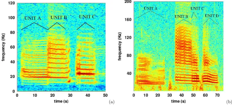
There are two blue whale song types in the southeast Pacific known as SEP1 and SEP2. SEP1 was first described almost fifty years ago [4], while SEP2 was first recorded in 1996 [24] near the Equator and described in detail as a new song type in 2014 [2]. In recent times, SEP2 has been found to be the dominant song type of southeast Pacific [3] [22]. These songs are composed of a single repeated phrase, highly stereotyped in unit composition, duration and frequency characteristics (see figure 1). SEP1 phrase is composed of 3 units [4] called A, B, C and shown in figure 1, left.

(a) (b)

Figure 1: (a) Time/frequency representation of a phrase of the SEP1 song, recorded in the Corcovado gulf, Chile, 2012 March 1st, sample rate fs=2 kHz, FFT 212 _{points, overlap of 90%, Blackman window. (b) Time/frequency} representation of a phrase of the SEP2 song, recorded off Isla Cha˜naral, Chile, 2nd February 2017, sample rate fs=48 kHz, FFT 216 _{points, overlap of 75%, Blackman window.}

SEP2 phrase is composed of 4 units [2] called A, B, C and D and shown in figure 1, right. The SEP2 phrase is usually repeated every two minutes, in a sequence lasting from some minutes to a few hours (called a song). All these features are observable only in clear recordings, with high signal to noise ratio (SNR). Units C and D are usually the loudest and together

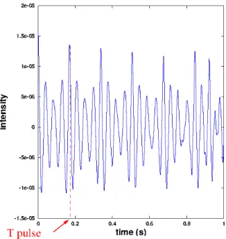
have been used as a kernel for automatic detection [3]. One of the defining characteristics of these song types is the pulsed nature

of their units, visible in figure 2 as a repetition rate at low frequency. The SEP1 units have a pulse rate fpulse around 6 pulses

per second for units B and C, and 3 pulses per second for unit A. The SEP2 units have a pulse rate fpulsearound 6 pulses per

second for units B, C and D, and 3 pulses per second for unit A (see part for measurements techniques). This pulse rate can also be seen as the frequency gap between two bands in figure 1 [29].

-0.01 0 0.01 0 0.2 0.4 0.6 0.8 1 Amplitude time (s) _(a) -0.02 -0.01 0 0.01 0.02 0 0.2 0.4 0.6 0.8 1 Amplitude time (s) _(b)

Figure 2: Extracts of units A (a) and C (b) of a SEP2 song recorded off Isla Cha˜naral, 2017 February the 2nd, in waveform.

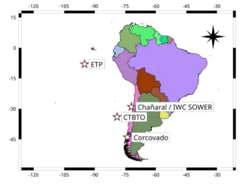
These song types have been recorded at different sites in the eastern Pacific Ocean: near the Equator, in the eastern tropical Pacific (ETP) between 1996 and 2002 [24], off the north coast of Chile in 1997-1998 by the International Whaling Commission’s Southern Ocean Whale and Ecosystem Research (IWC SOWER) program [23], in the Corcovado Gulf in the south of Chile in 2012, 2013, 2016, 2017 [3], near the Juan Fernandez archipelago off Chile in 2005, from 2007 to 2010 and from 2014 to 2016

by the Comprehensive Nuclear-Test-Ban Treaty Organization (CTBTO https://ctbto.org/) and off Isla Cha˜naral, Chile, in 2017

[20].

In this paper, we examine the frequency characteristics of the SEP song types by computing the pulse rate and peak frequency of their units to determine whether frequency decline has occurred in the last decades, using seven different data sets. We also discuss the sources of error associated with both pulse rate and peak frequency measurements.

Data collection

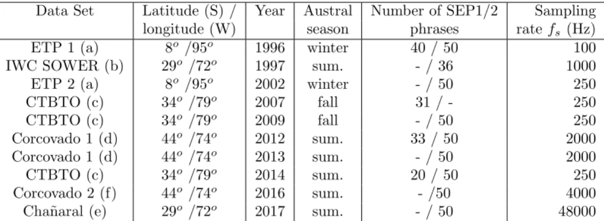
Because it is the predominant song type, we first analyzed in detail 436 SEP2 song phrases spanning 21 years (1996-2017), from 5 different locations and 7 different data sets listed in Table 1 and displayed in figure 3.

Fifty high SNR phrases were manually selected for each year. To minimize the probability of only analyzing phrases from a single song bout, phrases were taken from five different days. In the case of the SOWER data, only 36 phrases from three different days were selected, due to the short duration of the data set.

Data Set Latitude (S) / Year Austral Number of SEP1/2 Sampling

longitude (W) season phrases rate fs(Hz)

ETP 1 (a) 8o _/95o _{1996 winter 40 / 50 100}

IWC SOWER (b) 29o _/72o _{1997 sum. - / 36 1000}

ETP 2 (a) 8o _/95o _{2002 winter - / 50 250}

CTBTO (c) 34o _/79o _{2007 fall 31 / - 250} CTBTO (c) 34o _/79o _{2009 fall - / 50 250} Corcovado 1 (d) 44o _/74o _{2012 sum. 33 / 50 2000} Corcovado 1 (d) 44o _/74o _{2013 sum. - / 50 2000} CTBTO (c) 34o _/79o _{2014 sum. 20 / 50 250} Corcovado 2 (f) 44o _/74o _{2016 sum. - /50 4000}

Cha˜naral (e) 29o _/72o _{2017 sum. - / 50 48000}

Table 1: Characteristics of the data analyzed. Table includes name of the data set, references, place, season, number of phrases analyzed and sample rate of the data. References : (a) : Stafford et al. 1999[24], (b) Shabangu et al. 2018 [23], (c) CTBTO https://ctbto.org/ , (d) Buchan et al. 2015 [3], (e) Patris et al. 2017 [20], (f) : Buchan et al., unpublished The oldest data for SEP2 is 1996. For the SEP1 song type, however, first description was mentioned as far back as 1970 [4]. We were not able to have access to the raw data, however we made use of the results published in the paper, where only pulse rate, but not peak frequency is reported. Also, over all available data bases, there are fewer examples of SEP1. With these limitations, we applied the same approach for SEP2 to SEP1 examples to compute peak frequency and pulse rate and examine whether SEP1 has the same rate of decrease as SEP2. The number, location and season of the SEP1 occurrences analyzed are displayed in table 1. This allows us to examine SEP1 frequency shift over 44 years (1970-2014), which is double the time period available for SEP2, though with fewer data.

Data analysis

Methods

To estimate the frequency decrease, we measured the peak frequency and pulse rate of units of each phrase of SEP song types. Fast Fourier transform to measure the peak frequency

The spectral power density of whales’ vocalizations usually presents a set of discrete peaks. To measure the frequency trend of the song it is important to choose the peak consistently from one signal to the other. Strictly speaking, the so-called “peak frequency”

fpeak is the frequency of the peak with maximum energy ; this definition has been used for instance in [2]. However, the peak

where energy is maximum can be highly variable due to environmental effects or sensor sensitivity even though the general set of frequency peaks within a single unit is very stable at subdecadal timescales. Following [13] [6] [11], we decided to call ’peak frequency’ the frequency of the band that is on average the one with maximum energy, which in this case is around 25 Hz for the SEP song type. When maximum energy is shifted to the 32 Hz frequency band, we still measured the exact frequency of the band around 25 Hz, in order to ensure a standard metric for examining the decadal trend in the song frequencies.

For all selected units, we performed a FFT on the first 4 s of the unit by a routine in OCTAVE [5]. We measured the peak frequency as the frequency corresponding to the maximum value (in modulus) of the FFT between 23 and 26 for unit A of each song type and 22 and 27 Hz for the other units. Long term spectral averages [6] were not computed because of the complex nature of SEP songs compared, for example, to the Antarctic blue whale song type : the frequencies of different parts of the song overlap, blurring the long-term average.

Auto-correlation of the signal to measure the pulse rate

For SEP2, units are periodic, or harmonic, signals : the pulse rate (fpulse) is the fundamental frequency of these units and the

ratio fpeak

fpulse is an integer [21]. This ratio is equal to 8 for unit A and 4 for units B, C and D. For SEP1 units, we checked first that units B and C are harmonic (see section results bellow for details). In this case, the pulse rate can be accurately measured by an summed auto-correlation of the signal when the sample rate of the recording is high (see the following section, about associated uncertainties). The auto-correlation function of a signal s is

C(τ ) = limT →+∞ 1 T Z T /2 −T /2 s(t)s∗(t + τ )dt (1)

(where s∗is the complex conjugate of s). In practice, s is a real signal, time T is limited by duration Tsignalof the unit and

our signal is sampled at a frequency fs. We thus define an approximation of C(τ ) by

CTsignal,Ts(τ ) =

⌊TsignalX/Ts⌋

n=0

s(nTs)s(nTs+ τ ) (2)

where Ts= _f1_s is the sampling interval and ⌊x⌋ is the integer part of a real number x. Here, we have Tsignal= 4 s. If the

signal s is harmonic, the function C(τ ) has maximums when τ is a multiple of the period. For a description of auto-correlation techniques applied to mysticete sounds see for example [14].

For each unit, we computed the approximate auto-correlation function (using an OCTAVE dedicated routine) for τ ∈ [0 : tcorrel = 1 s] with a step of Ts (see figure 4). A low-pass filter (fifth order Butterworth with frequency cut-off at 150 Hz)

was applied before the auto-correlation to reduce high frequency noise. To obtain a maximum likelihood of the pulse frequency measurement, we performed a refinement of the correlation method [31], involving the computation of the summed auto-correlation function g(t) = t tcorrel ⌊tcorrelX/t⌋ n=1 CTsignal,Ts(nt) (3)

We computed this function for all values of t between 0 and tcorrel with a step Ts. This function has a peak for t equal to

the period. We thus measured the corresponding time Tpulseof the highest peak of the summed auto-correlation in the interval

t ∈ [0.15; 0.175] s (corresponding to frequencies between 5.71 and 6.66 Hz) which gives the frequency fpulse= _Tpulse1 .

Figure 4: Graph of the auto-correlation CTsignal,Ts(τ ) of unit C : the maximum of correlation for Tpulse ≃ 0.17 s corresponds to a frequency fpulse ≃ 6 Hz. The time Tsignal is 4 s.

Error in frequency estimation

Uncertainties arise from three main sources : the inherent error of each method (quantification error) in measuring fpulseand

fpeak, ambient noise and the intrinsic dispersion in whale vocalizations. We assessed separately these three causes of uncertainty

in the measurements.

• Uncertainties due to the method : quantification errors

Measuring peak frequency by means of a FFT cannot be more precise than the frequency step of the FFT (quantification

of the frequency). Given that useful parts of SEP units are around Tsignal= 4 s long, the highest resolution FFT that can

be computed is fs× Tsignal points. This results in a precision in frequency of _fs×Tfs

signal =

1

4 = 0.25 Hz. We note that this

uncertainty is 1/Tsignal and thus does not depend on the sampling rate fs.

On the other hand, the quantification error of the summed auto-correlation method depends strongly on fs. To estimate

fpulse, assuming that the recording device has a sample rate fs, the uncertainty in time ∆Tpulsewhen we measure Tpulse

∆Tpulse/Tpulse2 = fpulse2 ∆Tpulse≃ fpulse2 /fs. In the case of a sample rate of 48 kHz and for a measured frequency fpulse

around 6 Hz, the quantification error is ∆fpulse ≃ 10−3 Hz. But for fs = 2 kHz, we have ∆fpulse ≃ 0.05 Hz and for

fs= 100 Hz, we have ∆fpulse≃ 0.2 Hz.

We can also compute (and compare) the relative quantification error ∆f /f . For our signals, we have fpulse≃ 6 Hz and

fpeak≃ 24 Hz. The relative error of fpeakmeasurement is thus ∆fpeak/fpeak= 1/(Tsignal×fpeak) ≃ 1% for each recording.

The relative error of fpulsemeasurement depends on the sample rate: ∆fpulse/fpulse= fpulse/fs. It becomes smaller than

1% for fs greater than 400 Hz (fs = 100 Hz leads to ∆fpulse/fpulse ≃ 6%,fs = 2000 Hz leads to ∆fpulse/fpulse ≃

0.3%). Thus, pulse rate measurement has a smaller systematic relative uncertainty than peak frequency measurement for

fsgreater than 400 Hz.

• Uncertainty due to noise

To compute SNR, the following approach was used: The energy of a unit of duration Tsignalis proportional toR₀Tsignal|s(t)|2dt

[1]. We computed an approximation of the energy (where the coefficient A depends on the sampling rate but is constant for a given signal and will not appear in the SNR) :

ESEP2= A

⌊TsignalX/Ts⌋

n=0

|s(nTs)|2

We measured the energy of each unit by computing the energy E of the signal during 4 s. A band-pass filter (fifth order Butterworth with frequency band 5-50 Hz) was applied before the computation of energy. We then calculated the SNR by

estimating the energy EN of the background noise at a time selected manually before or after each SEP2 phrase, using

the same formula and during the same Tsignal. We compute SN R(dB)= 10 log10(ESEP2EN ) for each SEP2 song phrase. The

SNR varied from 1 dB to 40 dB in the 436 selected SEP2 phrases.

To check each method’s resistance to noise, we selected one song from the 14th of February 2012 in Corcovado with high SNR (around 40 dB) and we added background noise (taken from the same recording) with increasing level, resulting in a deterioration of the SNR. We then measured the peak frequency and pulse rate.

The measurement of peak frequency by means of a FFT was robust despite increasing background noise: for all levels of noise measured, the main error in the measurement comes from the quantification error. The main noises in the recordings were : short-duration (less than 1s) low frequency (less than 30-40 Hz) sounds that are especially strong in bad weather and long tonal sounds from ship motors. As the FFT is a linear process and signal to noise ratios were sufficiently high, these sounds did not prevent us from accurately measuring peak frequency. As for the measurement of the pulse rate, these noises seemed to have a higher influence on measurement, probably given that auto-correlation is a non-linear process.

By performing several measurements of fpulsefor different noise levels, we estimated the uncertainties, which were on the

order of 0.05 Hz or less, and shown as error bars in figures 5 and 6. • Intrinsic dispersion of frequencies

In theory, intrinsic dispersion is due to the difference between two different sounds emitted by two different whales; two different sounds emitted by the same whale; or two sounds emitted by the same whale but affected differently by propagation

effects. For example, in the latter case, the Doppler effect changes the received frequency by freceived = _1−v/c1 × femitted

where c is the sound speed and v is the radial speed of the whale relative to the recording device. For a typical value of v/c ≃ 1/1000, the difference in the frequency estimation is of the order of 0.1%. That is, for a frequency of 25 Hz, a difference of 0.025 Hz is obtained (see [17] for a detailed analysis). Dispersion uniquely caused by sound production (the former two cases) is extremely difficult to estimate and seems very small [8].

To estimate the intrinsic dispersion, regardless of its cause, we computed the standard deviation of results obtained for

each year for fpeak and fpulse. This standard deviation can also be affected by the two precedent sources of uncertainty

(background noise and quantification of measurements). These different causes of uncertainty can be separated theoretically. In the data, they are usually not separable. However, in some instances they appear clearly, as for instance when standard deviation is zero due to quantification errors (quantification errors are then masking the intrinsic dispersion).

• Representation of uncertainties

For each year, we computed the quantification error, the error due to noise and the standard deviation of measured values, and we chose the greater of the three values to represent errors graphically (see figures 5 and 6).

Results

Application to SEP2

As presented in the section about data analysis, we measured peak and pulse frequencies for the four units of 436 SEP2 phrases. The measure of theses frequencies for units A and B did not give precise results since theses units usually have lower SNR and are somewhat modulated in frequency (see figure 1). Only measurements of units C and D are analyzed in the following.

Shift in peak frequency

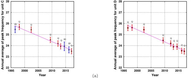
Figure 5 clearly shows the decrease in peak frequency for the two units C and D between 1996 and 2017. As found for other blue whale song types [13], the shift in frequency seems to be linear over time.

22 23 24 25 26 27 28 1995 2000 2005 2010 2015

Annual average of peak frequency for unit C

Year ID ID ID Q Q Q Q Q Q (a) 22 23 24 25 26 27 28 1995 2000 2005 2010 2015

Annual average of peak frequency for unit D

Year Q Q Q Q Q Q Q Q Q (b) Figure 5: Temporal evolution of the peak frequency of units C (a) and D (b), computed by a Fast Fourier transform of the signal. The error bars color code is : red when quantification error is the greatest source of error, blue when intrinsic dispersion is the greatest source of error. A letter corresponding to the largest source of error is given on top of each error bar. The line is the linear interpolation by least-square error of the points displayed in the graph (the coefficient of determination R2 _{being close to 0.95).}

The peak frequency of unit C dropped from 25.8 ±0.25 Hz in 1996 to 23.6 ±0.25 Hz in 2017, an average decrease of 0.10 ±0.03 Hz per year. For unit D, peak frequency dropped from 25.8 ±0.25 Hz in 1996 to 23.5 ±0.25 Hz in 2017, resulting in a decrease of 0.11 ±0.03 Hz per year. For almost all years, the main source of uncertainty was quantification error. This means that this method has reached its intrinsic limit of precision for analyzing this type of sound.

Shift in pulse rate

Figure 6 displays the pulse rate for SEP2 blue whale song type over 20 years, from 1997 to 2017. The results for 1996 were not plotted because auto-correlation methods produced unreasonable values due to the very low sample rate of these

recordings, (fs = 100 Hz). In general, the relative error for pulse rate measurements was higher than for peak frequency

measurements, although quantification errors can be reduced (typically with a higher sample rate of recording) for pulse rate measurement but not for peak frequency. Recordings with a high sample rate and high SNR usually had lower associated uncertainty (eg. years 2012 and 2013). Moreover, calculating an average reduces the uncertainty when error is introduced due to noise or intrinsic dispersion, but it usually does not reduce the error due to quantification.

The decrease also appears linear for the pulse rate. This is consistent with a harmonic signal and the fixed ratio fpeak

fpulse. The pulse rate of unit C dropped from 6.44 ±0.06 Hz in 1997 to 5.87 ±0.10 Hz in 2017, an average decrease of 0.03 ±0.01 Hz per year. For unit D, the pulse frequency dropped from 6.45 ±0.06 Hz in 1997 to 5.87 ±0.10 Hz in 2017, resulting in a decrease of 0.03 ±0.01 Hz per year.

Application to SEP1 and results

First, we checked if SEP1 units were harmonic or not by computing the values of fpeak and fpulsefor forty SEP1 phrases

with high SNR selected from the 2012 and 2014 data sets[21]. fpulsewas measured by an auto-correlation of the envelope

of the signal. We found that fpeak

fpulse = 6.23 ± 0.50 for unit A, 3.06 ± 0.09 for unit B and 4.07 ± 0.09 for unit C. We thus assumed that the peak frequency of units B and C is an integer multiple of the pulse rate (as for units of SEP2) and therefore SEP1 units B and C are also harmonic. We then measured both pulse rate (by summed auto-correlation of the signal as presented in section about data analysis) and peak frequency of 107 high SNR units B and C of SEP1 selected from four years of data (see table 1). We also took the value of the pulse rate for 1970 given in the literature [4]. We did not have access to the precise values of peak frequencies for 1970 because in this paper peak frequencies are given only at a precision of 1/3 octave. For 1996, the low sampling rate (100 Hz) did not enable us to make a precise measure of the

pulse rate. Considering than fpeak

fpulse = 3 for unit B and

fpeak

fpulse = 4 for unit C, we estimated the long term decline of fpulse combining both methods (see figure 7).

5.4 5.6 5.8 6 6.2 6.4 6.6 6.8 1995 2000 2005 2010 2015

Annual average of pulse rate for unit C

Year Q Q N ID IDQ ID N (a) 5.4 5.6 5.8 6 6.2 6.4 6.6 6.8 1995 2000 2005 2010 2015

Annual average of pulse rate for unit D

Year N Q Q Q ID_ID ID ID (b) Figure 6: Evolution of the pulse rate of units C (a) and D (b). Error bars are red when quantification error is the greatest source of error, green when error due to the noise is the greatest source of error, blue when intrinsic dispersion is the greatest source of error. A letter corresponding to the largest source of error is given on top of each error bar. The line is the linear interpolation by least-square error of the points displayed in the graph (the coefficient of determination R2 _{being close to 0.98).}

The decrease is clearly linear for pulse rate of units B and C and is of 0.029 ± 0.005 Hz/year and 0.037 ± 0.005 Hz/year respectively, which compares well with SEP2 (unit C: 0.03 ± 0.01 Hz/year and unit D: 0.03 ± 0.01 Hz/year). Interestingly, the two units B and C of the SEP1 song types are not decreasing at the same rate. In 1970, these two units were quite similar in term of frequencies [4]. Since then, the two fundamental frequencies have decreased at a different rate and each unit appear nowadays quite different in time-frequency representation, see figure 1. Although SEP1 and SEP2 have similar time and frequency characteristics, and appear to occur with the same temporal distribution [3], it remains unclear whether these songs types indicate the presence of one or two acoustic groups.

Comparison with frequency shifts in other regional song types

To compare our results with other frequency shifts that have been reported, we extracted data about peak frequency from published papers (See Table 2). Several song types do not present pulsed units. Therefore a comparison of pulse rates is not relevant in this case. Nevertheless a clarification, for each pulsed unit of each song type, of the link between the fundamental frequency and the pulse rate could enable to understand better each song type, its production and to realize better measures of frequency trends.

For the different song types, the values of the peak frequencies are very different (many of them are around 20 Hz but other are around 30 Hz and, in the north of Indian Ocean, it is near 100Hz). Thus, to compare different data, we computed the absolute values of the average decrease of the peak frequency during one year as % of the value estimated in a reference year. We chose the year 2000 as reference year and calculated, for each song type, the mean value of the peak frequency during this year, by linear interpolation. The results are presented in table 2.

The frequency decrease observed here in SEP2 song types is comparable to that of other song types reported in the table 2. Interestingly, all song types from the north and west Pacific Ocean have a greater decrease than songs from other oceans and song types from the Indian Ocean have a smaller decrease than in other oceans.

Two different decreases are given for the southeast and north Indian ocean because two different units of the same song type have been measured. Recently, the last two units of the North Indian song type has been proved to decrease at different rates as in our study about SEP1 units B and C [15]. Studies have shown that several blue whale song types have intra-annual variations[6] [16] [11]. In our case we do not have such temporal precision and we cannot see these seasonal changes, which are masked by our error bars in figures 5 and 6.

Discussion and conclusion

We observed a linear frequency shift that is very similar to other blue whale song frequency shifts in both SEP1 and SEP2 song types. We note that depending on the data, either peak frequency or pulse rate measurements can be used for these units and give similar results. Error analysis shows that for data with a high sample rate (higher than 400 Hz), the pulse rate measurement with summed auto-correlation method has the best precision. In the case where occurrences of a song type are scarce and several data sets are used, the combination of these two methods can give a better understanding of

5.5 6 6.5 7 7.5 8 8.5 1965 1975 1985 1995 2005 2015

Annual average of pulse frequency for unit B of SEP1

Year _(a) 5.5 6 6.5 7 7.5 8 8.5 1965 1975 1985 1995 2005 2015

Annual average of pulse frequency for unit C of SEP1

Year _(b)

Figure 7: Pulse rate decrease in SEP1 phrases units. In blue (circles) the measures of pulse rate by mean of a summed auto-correlation method except the value of 1970 which is taken from literature [4]. In red (crosses), the points are computed by estimation of the frequency peak (by a FFT) divided by 3 and 4 for units B and C respectively (figures (a) and (b)). The errors bars are computed as for SEP2. The line is the linear interpolation by least-square error of the points displayed in the graph.

the trend. Nevertheless, we have to be cautious with the long-term analysis of SEP1 frequencies due to the small number of SEP1 occurrences analyzed (only 5 data points).

Fin whales emit song types composed of short low frequency sounds around 20 Hz usually named “pulses” [30]. These sounds are repeated at a nearly constant rate which is also called “pulse rate” in the literature. A joint decrease of the pulse rate and peak frequency, at a different rate, has been recently noticed for fin whales songs in the northeast Pacific Ocean [28]. Decrease in peak frequency of fin whales calls in the Indian Ocean have been described by [11]. Decrease of fin whales pulse rates have also been described in north Atlantic Ocean [18] and in northeast Pacific Ocean [26]. A frequency decrease has been found in an unidentified baleen whale “spot call” [27], with sudden increase of peak frequency after some years of constant decrease. This unidentified baleen whale may be a southern right whale [27]. This similarity between blue whales and other species sound emissions trends (pulse rate and frequency decrease over years) has to be addressed, since it is undoubtedly part of the worldwide question of whales song frequency decline.

Future studies of frequency trends of song types of baleen whales should measure both peak frequency and pulse rate when it is possible. A precise value of pulse rate can be obtained whenever the signal is harmonic, the sampling rate is high enough and the SNR good. And it is specially relevant to measure it when the sound is low frequency and not long compared to the pulse duration, as in most of blue whale song types.

References

[1] Au, W., and Hastings, M. (2008). Principles of marine bioacoustics (Springer).

[2] Buchan, S., Hucke-Gaete, R., Rendell, L., and Stafford, K. (2014). “A new song recorded from blue whales in the

corcovado gulf, southern chile, and an acoustic link to the eastern tropical pacific,” Endangered Species Research 23, 241–252.

[3] Buchan, S., Stafford, K., and Hucke-Gaete, R. (2015). “Seasonal occurrence of southeast pacific blue whale songs

in southern chile and the eastern tropical pacific,” Marine Mammal Science 31(2), 440–458.

[4] Cummings, W., and Thompson, P. (1971). “Underwater sounds from the blue whale, balaenoptera musculus,”

Jour-nal of the Acoustical Society of America (50), 1193–1198.

[5] Eaton, J. W., Bateman, D., and Hauberg, S. (2009). GNU Octave version 3.0.1 manual: a

high-level interactive language for numerical computations (CreateSpace Independent Publishing Platform),

http://http://www.gnu.org/software/octave/doc/interpreterhttp://www.gnu.org/software/octave/doc/interpreter, ISBN 1441413006.

[6] Gavrilov, A., McCauley, R., and Gedamke, J. (2012). “Steady inter and intra-annual decrease in the vocalization

frequency of antarctic blue whales,” J. Acoust. Soc. Am. 131(6), 4476–4480.

[7] Gavrilov, A., McCauley, R., Salgado-Kent, C., Tripovitch, J., and Wester, C. B. (2011). “Vocal characteristics of

Song Period Frequency Decrease in % of

type studied (Hz) 2000’s value / year

Northeast Pacific (a) 1963-2008 21.9 to 15.2 0.91

Southwest Pacific (a,d) 1964-2013 25.3 to 17.5 0.81

Northwest Pacific (a) 1968-2001 23.0 to 17.9 0.86

North Atlantic (a) 1959-2004 23.0 to 17.6 0.66

Southern Ocean (a,c,e,f ) 1995-2014 28.5 to 25.8 0.50

North Indian (unit 2) (g) 2002-2012 61.5 to 59.8 0.27

North Indian (unit 3) (a,f,g) 1984-2013 116 to 99.5 0.51

Southeast Indian (unit 2) (b) 2002-2010 72.5 to 69.5 0.51

Southeast Indian (unit 3) (a) 1993-2000 19.5 to 19.0 0.38

West Indian (f ) 2007-2015 34.7 to 33.7 0.35

Southeast Pacific 1 (unit B) 1970-2014 23.1 to 19.3 0.43

Southeast Pacific 1 (unit C) 1970-2014 30.8 to 24.3 0.58

Southeast Pacific 2 (unit C) 1996-2017 25.8 to 23.6 0.44

Southeast Pacific 2 (unit D) 1996-2017 25.8 to 23.5 0.45

Table 2: Comparison of our results to other works. (a) McDonald et al. 2009 [13] (b) Gavrilov et al. 2011 [7] (c) Gavrilov et al. 2012 [6] (d) Miller et al. 2014 [16] (e) Leroy et al. 2016 [9] (f )Leroy et al. 2018 [11] (g) Miksis et al. 2018 [15]

.

[8] Hoffman, M., Garfield, N., and Bland, R. (2010). “Frequency synchronization of blue whale calls near pioneer

seamount,” The Journal of the Acoustical Society of America 128(1), 490–494 doi:10.1121/1.3446099.

[9] Leroy, E., Samaran, F., Bonnel, J., and Royer, J.-Y. (2016). “Seasonal and diel vocalization patterns of antarctic

blue whale (balaenoptera musculus intermedia) in the southern indian ocean: A multi-year and multi-site study,” PLoS ONE 11(11): e0163587. doi:10.1371/journal.pone.0163587 .

[10] Leroy, E. C., Samaran, F., Bonnel, J., and Royer, J.-Y. (2017). “Identification of two potential whale calls in the southern indian ocean, and their geographic and seasonal occurrence,” The Journal of the Acoustical Society of America 142, 1413–1427.

[11] Leroy, E. C., Royer, J.-Y., Bonnel, J., and Samaran, F. (2018). “ Long Term and Seasonal Changes of Large Whale Call Frequency in the Southern Indian Ocean,” Journal of Geophysical Research: Oceans 123, 8568–8580.

[12] McDonald, M., Mesnik, S., and Hildebrand, J. (2006). “Biogeographic characterization of blue whale song worldwide: using song to identify populations,” J. Cetacean Res. Manage. .

[13] McDonald, M., Hildebrand, J., and S.Mesnick (2009). “Worldwide decline in tonal frequencies of blue whale songs,” Endangered species research 9, 13–21.

[14] Mellinger, D., and Clark, C. W. (1997). “Methods for automatic detection of mysticete sounds,” Marine and Fresh-water Behaviour and Physiology 29: 1-4, 163–181.

[15] Miksis-Olds, J. L., Nieukirk, S. L., and Harris, D. V. (2018). “Two unit analysis of Sri Lankan pygmy blue whale song over a decade,” J. Acoust. Soc. Am. 144(6).

[16] Miller, B. S., Collins, K., Barlow, J., Calderan, S., Leaper, R., McDonald, M., Ensor, P., Olson, P., Olavarria, C., and Double, M. (2014a). “Blue whale vocalizations recorded around new zealand : 1964-2013,” J. Acoust. Soc. Am. 135(3), 1616–1623.

[17] Miller, B., Leaper, R., Calderan, S., and Gedamke, J. (2014b). “Red shift, blue shift : Doppler shifts and seasonal variation in the tonality of antarctic blue whale song,” PLoS ONE 9(9): e107740. doi:10.1371/journal.pone.0107740 .

[18] Morano, J., Salisbury, D., Rice, A., Conklin, K., Falk, K., and Clark, C. (2012). “Seasonal and geographi-cal patterns of fin whale song in the western north atlantic ocean,” J. Acoust. Soc. Am. 132(2), 1207–1212 http://dx.doi.org/10.1121/1.4730890.

[19] Oleson, E. M., Calambokidis, J., Burgess, W. C., McDonald, M. A., LeDuc, C. A., and Hildebrand, J. A. (2007). “Behavioral context of call production by eastern north pacific blue whales,” Mar Ecol Prog Ser 330, 269–284.

[20] Patris, J., Malige, F., and Glotin, H. (2017). “Construction et mise en place d’un syst`eme fixe d’enregistrement `a

large bande pour les c´etac´es “bombyx 2” isla de cha˜naral, ´et´e austral 2017,” Technical Report, LIS DYNI, Toulon

[21] Patris, J., Malige, F., Glotin, H.,Asch, M. and Buchan, S. J. (2019). “A standardized method of classifying pulsed sounds and its application to pulse rate measurement of blue whale southeast Pacific song units,” J. Acoust. Soc. Am..

[22] Saddler, M., Bocconcelli, A., Hickmott, L. S., Chiang, G., Landea-Briones, R., Bahamonde, P. A., Howes, G., Segre, P. S., and Sayigh, L. S. (2017). “Characterizing chilean blue whale vocalizations with dtags : a test of using tag accelerometers for caller identification,” Journal of Experimental Biology 220, 4119–4129 doi:10.1242/jeb.151498. [23] Shabangu, F., Stafford, K., Findlay, K., Rankin, S., Ljungblad, D., Tsuda, Y., Morse, L., Clark, C., Kato, H., and

Ensor, P. (2018). “Overview of the iwc sower cruise circumpolar acoustic survey data and analyses of antarctic blue whale calls within the dataset,” Technical report.

[24] Stafford, K. M., Nieukirk, S. L., and Fox, C. G. (1999). “Low-frequency whale sounds recorded on hydrophones moored in the eastern tropical pacific,” J. Acoust. Soc. Am. 106(6), 3687–3698.

[25] Thode, A. M., Blackwell, S. B., Conrad, A. S., Kim, K. H., and Macrander, A. M. (2017). “Decadal-scale frequency shift of migrating bowhead whale calls in the shallow beaufort sea,” J. Acoust. Soc. Am. 142(3).

[26] ˇSirovi´c, A., Oleson, E., Buccowich, J., Rice, A., and Bayless, A. R. (2017). “Fin whale song variability in southern

california and the gulf of california,” Scientific reports 7 dOI:10.1038/s41598-017-09979-4.

[27] Ward, R., Gavrilov, A., and McCauley, R. (2017). ““spot” call: A common sound from an unidentified great whale in australian temperate waters,” J. Acoust. Soc. Am. Express Letters 142 http://dx.doi.org/10.1121/1.4998608. [28] Weirathmueller, M. J., Stafford, K. M., Wilcock, W. S. D., Hilmo, R. S., Dziak, R. P., and Trehu, A. M. (2017).

“Spatial and temporal trends in fin whale vocalizations recorded in the ne pacific ocean between 2003-2013,” PLOS ONE 12(10) https://doi.org/10.1371/journal.pone.018612.

[29] Watkins, W., ed. (1968). The Harmonic interval fact or artifact in spectral analysis of pulse train, 2 (Pergamon Press-Oxford and New-York, American Museum of Natural History, New York).

[30] Watkins, W. A., Tyack, P., Moore, K. E., and Bird, J. E. (1987). “The 20-Hz signals of finback whales (Balaenoptera physalus),” J. Acoust. Soc. Am. 82(6)

[31] Wise, J., Caprio, J., and Parks, T. (1976). “Maximum likelihood pitch estimation,” in Transactions on acoustics, speech and signal processing, edited by IEEE, Vol. ASSP-24.

Acknowledgements

The authors thank the help of Explorasub diving center (Chile), Agrupaci´on tur´ıstica Cha˜naral de Aceituno (Chile),

ONG Eutropia (Chile), Valparaiso university (Chile), the international institutions and research programs CTBTO, IWC, BRILAM STIC AmSud 17-STIC-01. S.J.B. thanks support from the Center for Oceanographic Research COPAS Sur-Austral, CONICYT PIA PFB31, Biology Department of Woods Hole Oceanographic Institution, the Office of Naval Research Global (awards N62909-16-2214 and N00014-17-2606), and a grant to the Centro de Estudios Avanzados en

Zonas ´Aridas (CEAZA) “Programa Regional CONICYT R16A10003”. We thank SABIOD MI CNRS, EADM MaDICS

CNRS and ANR-18-CE40-0014 SMILES supporting this research. We are grateful to colleagues at DCLDE 2018 and SOLAMAC 2018 conferences for useful comments on the preliminary version of this work. In this work we used only the free and open-source softwares Latex, Audacity and OCTAVE.

Author contributions statement

F.M. and J.P. did most of the analysis presented. They wrote the paper with S.J.B. who contacted the authors and gathered all the recordings used. H.G participated in the redaction of the paper and in the analysis. K.S. and F.S. participated in the redaction of the manuscript. K.S, F.S, K.F, R.H-G., S.N. and C.W.C set up experiments to record blue whale vocalizations in the Southeast Pacific. All authors reviewed the manuscript.