HAL Id: tel-03209390
https://tel.archives-ouvertes.fr/tel-03209390
Submitted on 27 Apr 2021
HAL is a multi-disciplinary open access
archive for the deposit and dissemination of sci-entific research documents, whether they are pub-lished or not. The documents may come from
L’archive ouverte pluridisciplinaire HAL, est destinée au dépôt et à la diffusion de documents scientifiques de niveau recherche, publiés ou non, émanant des établissements d’enseignement et de
Hydro Power Plant Applications.
Thomas Lugand
To cite this version:
Thomas Lugand. Contribution to the Modeling and Optimization of the Double-Fed Induction Ma-chine for Pumped-Storage Hydro Power Plant Applications.. Electric power. Université de Grenoble, 2013. English. �NNT : 2013GRENT118�. �tel-03209390�
DOCTEUR DE L’UNIVERSITÉ DE GRENOBLE
Spécialité : Génie Électrique
Arrêté ministériel : 7 aout 2006
Présentée par
Thomas LUGAND
Thèse dirigée par Gérard Meunier et codirigée par Albert Foggia
préparée au sein du Laboratoire de Génie Électrique de Grenoble
(G2Elab)
et de l’École Doctorale Électronique, Électrotechnique, Automatique
et Traitement du Signal (EEATS)
Contribution to the Modeling and Optimization
of the Double-Fed Induction Machine for
Pumped-Storage Hydro Power Plant Applications
Thèse soutenue publiquement le 2 décembre 2013, devant le jury composé de :
Christophe ESPANET
Professeur à l’université de Franche-Comté, Président
Mohamed BENBOUZID
Professeur à l’université de Brest, Rapporteur
Yvan LEFEVRE
Chargé de Recherche au CNRS de Toulouse, Rapporteur
Alexander SCHWERY
Directeur R&D Électrique chez ALSTOM Renewable Power Switzerland, Examinateur
Albert FOGGIA
Professeur Émérite à Grenoble-INP, Co-Directeur de thèse
Gérard MEUNIER
I would like to thank Alexander Schwery, R&D Electrical Director at Alstom Renewable who proposed me this thesis subject and who gave me the chance to work in his department. I would like to express my sincere gratitude to Albert Foggia, Professor at Grenoble-INP and Gérard Meunier, Senior Researcher at Grenoble CNRS, for their support and for having super-vised my work.
I would like to thank all the members of the jury, Christophe Espanet, Professor at Franche-Comté University, Mohamed Benbouzid Professor at Brest University and Yvan Lefevre, Re-searcher at Toulouse CNRS for taking time to study and to review my work.
I am very grateful to my former colleague Georg Traxler-Samek as well as my colleagues from Alstom Birr, Carlos Ramirez and Glenn Ardley for their help and for sharing their experience about electrical machines.
I would like to thank Hans Werner Lorenzen, Professor at TU Munich, for his help and for sharing his experience about the double-fed induction machine.
I would like to thank Afef Lebouc, Senior Researcher at Grenoble CNRS, for sharing her expe-rience about magnetic material modeling.
I am very grateful to Daho Taghezout from the company applied magnetics for his support and advices relative to electrical machines and finite element computations.
I would like to express my sincere gratitude to my colleagues from Global Technology Centre in Alstom Birr, in particular Peter Tönnies for his help with LATEX, as well as all the personnel from Grenoble Electrical Engineering Laboratory for their support and for their kindness. I would like to thank my friends for their support and in particular Bénédicte, Bernard, Jonathan, Nathanael and Michael for the good moments in Grenoble.
Finally I would like to thank my parents and Christina for their support as well as my little Lara for the perfect timing.
List of Figures ix
List of Tables xv
Acronyms xvii
1 Introduction 1
1.1 Regulating Power by using Pumped-Storage Hydro Power Plants . . . 1
1.2 Benefits of using Variable Speed for PSP applications . . . 2
1.2.1 Better Control of the power in pumping mode . . . 3
1.2.2 Work at the best operation point in turbine mode . . . 3
1.2.3 Better tracking of the power . . . 4
1.2.4 Better stabilization after a perturbation . . . 6
1.3 Variable speed technologies . . . 6
1.3.1 The changeable/commutable salient-pole synchronous machine . . . 8
1.3.2 The salient-pole synchronous machine connected to a static converter . . 9
1.3.3 The Brushless-Double-Fed Induction Machine . . . 9
1.3.4 The Double-Fed Induction Machine . . . 12
1.3.5 Summary . . . 15
1.4 Description and motivation of the study . . . 15
1.4.1 Restriction of the study domain . . . 15
1.4.2 Definition and motivation of the study . . . 16
1.4.3 Structure of the thesis . . . 17
2 Magnetic circuit model 19 2.1 Introduction . . . 19
2.2 The analytical magnetic model . . . 19
2.2.1 The Ampere-Maxwell theorem . . . 19
2.2.2 The magnetizing voltage and flux . . . 20
2.2.3 The magnetic saturation coefficient . . . 22
2.2.4 The magnetic drop calculation . . . 25
2.2.5 Calculation of the no-load characteristics . . . 29
2.3 Validation of the method . . . 29
2.3.1 The Two-dimensional finite element model . . . 29
2.3.3 Stator and rotor teeth flux density . . . 32
2.4 Conclusion . . . 36
3 Steady-state model 37 3.1 Introduction . . . 37
3.2 Structure of the equivalent scheme . . . 37
3.2.1 The magnetizing inductance . . . 38
3.2.2 The stator and rotor resistances . . . 38
3.2.3 The stator and rotor winding leakage inductance . . . 43
3.2.4 Validation with FE method . . . 49
3.2.5 Summary . . . 53
3.3 Steady-state study . . . 54
3.3.1 Power balance . . . 54
3.3.2 Calculation of a load operation point . . . 56
3.3.3 Parametric study . . . 60
3.4 Validation by finite element computations . . . 69
3.4.1 Modeling using a magneto-harmonic application . . . 70
3.4.2 Modeling using a time stepping application . . . 73
3.4.3 Comparison of results . . . 80
3.5 Conclusion . . . 81
4 Airgap harmonics model 82 4.1 Introduction . . . 82
4.2 Rotor and stator flux density with a constant airgap . . . 83
4.2.1 Definition of the mmf of a three-phase winding . . . 83
4.2.2 Definition of the stator and rotor magneto-motive-forces . . . 87
4.3 Calculation of the airgap permeance function . . . 89
4.3.1 Definition of the airgap permeance . . . 89
4.3.2 The slot ripple harmonics . . . 89
4.3.3 Numerical computation of the permeance . . . 91
4.4 Computation of the airgap flux density . . . 99
4.4.1 Definition of the airgap flux density . . . 99
4.4.2 Impact of magnetic saturation . . . 100
4.4.3 Airgap transformation factor and airgap flux density at the bore diameter 105 4.5 Potential improvement of the method . . . 108
4.5.1 Modeling of the stator and rotor core . . . 108
4.5.2 Connection of the stator and rotor core through the airgap . . . 113
4.5.3 Solving of the system . . . 114
4.5.4 Results . . . 115
5 Applications to the study of the electromagnetic behavior 122
5.1 Introduction . . . 122
5.2 The stator voltage harmonics . . . 123
5.2.1 Finite Element studies . . . 123
5.2.2 Analytic study . . . 129
5.2.3 Effect of the slip . . . 134
5.2.4 Effect of the rotor voltage source harmonics . . . 135
5.2.5 Summary . . . 140
5.3 The electromagnetic radial forces . . . 141
5.3.1 Identification of the dangerous radial forces . . . 142
5.3.2 Application to a fractional slot winding machine . . . 155
5.3.3 Winding optimization . . . 169
5.3.4 Summary . . . 179
5.4 The parasitic dynamic torques . . . 180
5.4.1 Finite element computation of the electromagnetic torque . . . 180
5.4.2 Shaft line modal analysis . . . 188
5.4.3 Study of the start up . . . 191
5.4.4 Summary . . . 195
5.5 The iron losses in stator and rotor core . . . 196
5.5.1 State of the art . . . 196
5.5.2 Analytical model for iron losses computation . . . 197
5.5.3 Analytical calculation of the flux density loci . . . 205
5.5.4 Analytical calculation of iron losses and comparison with Finite-Element . 209 5.5.5 Summary . . . 214
5.6 Conclusion . . . 214
6 Application to the dimensioning of the double-fed induction machine 215 6.1 Introduction . . . 215
6.2 Rated characteristics and dimensioning of a double-fed induction machine . . . . 215
6.2.1 Choice of the rated characteristics . . . 215
6.2.2 Choice of the main dimensions . . . 216
6.3 Dimensioning by solving an optimization problem . . . 222
6.3.1 Definition of the objective function . . . 222
6.3.2 Definition of the constraints . . . 222
6.3.3 Definition of the optimization algorithm . . . 223
6.4 Application to the conversion of a synchronous machine to a double-fed induction machine . . . 224
6.4.1 Only the rotor is replaced . . . 225
6.4.2 The rotor and stator are both re-designed . . . 230
7 Final conclusion and perspectives 236
7.1 Final conclusion . . . 236 7.2 Perspectives . . . 237
Nomenclature 238
1.1 Global Cumulative Installed Wind Capacity 1996-2012 . . . 1
1.2 PSP structure . . . 2
1.3 World wide expansion of PSP and nuclear activity . . . 3
1.4 Salient Pole synchronous machine and turbine . . . 4
1.5 Pump characteristics example . . . 5
1.6 Pump and Turbine characteristics example . . . 5
1.7 Relative turbine efficiency for fixed and variable speed . . . 6
1.8 Power tracking in turbine mode . . . 7
1.9 Fixed and variable speed dynamic behavior . . . 7
1.10 Dahlander couplings . . . 8
1.11 Commutable SP: Three possible configurations . . . 10
1.12 Salient poles synchronous machine with converter . . . 11
1.13 DFIM with cyclo-converter . . . 12
1.14 DFIM with VSI converter . . . 13
1.15 Cross section of the two machines . . . 14
1.16 Longitudinal section of the two machines . . . 14
2.1 Magnetic circuit . . . 20
2.2 Airgap flux density at different magnetizing states . . . 22
2.3 Form factor C1 . . . 24
2.4 Pole enclosure coefficient αi . . . 24
2.5 Modified magnetic characteristic curve in the teeth . . . 27
2.6 Stator slot geometry with different sections (not real proportions) . . . 28
2.7 Two-Dimensional Finite Element (2DFE) model . . . 30
2.8 Axial overview of the stator and rotor air ducts . . . 30
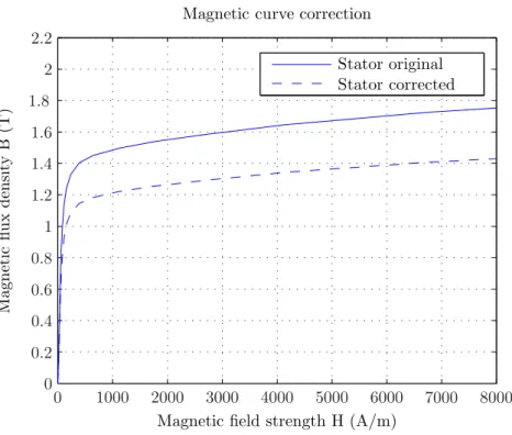
2.9 Correction of the material magnetic characteristic . . . 32
2.10 Magnetizing voltage: comparison between analytical method and FEM (design 1) 33 2.11 Magnetizing voltage: comparison between analytical method and FEM (design 2) 33 2.12 Stator flux density: comparison between analytical method and FEM (design 1) 34 2.13 Rotor flux density: comparison between analytical method and FEM (design 1) . 34 2.14 Stator flux density: comparison between analytical method and FEM (design 2) 35 2.15 Rotor flux density: comparison between analytical method and FEM (design 2) . 35 3.1 Equivalent scheme of the Double-Fed Induction Machine (DFIM) . . . 38
3.3 Slot with full bars (left) and subdivided bars (right) . . . 40
3.4 Rotor electrical frequency during startup . . . 40
3.5 Current density (left) and magnetic field (right) in a slot . . . 41
3.6 Roebel bar technology (patent: Ludwig Roebel 1912) . . . 42
3.7 Detailed slot geometry with only one conductor . . . 44
3.8 Detailed slot geometry with two conductors . . . 45
3.9 magneto-motive force (mmf) distribution of a three-phase winding . . . 46
3.10 Airgap flux leakage example . . . 47
3.11 Example of end-winding coils . . . 52
3.12 Three-dimensional finite element end-winding model . . . 52
3.13 Electrical circuit for end-winding inductance calculation . . . 53
3.14 Power exchange for Cyclo-converters (left) and VSI (right) topologies . . . 55
3.15 Load point calculation algorithm 1 . . . 58
3.16 Vector diagrams in generator mode . . . 61
3.17 Vector diagrams in motor mode . . . 61
3.18 Influence of the slip on rotor voltage . . . 62
3.19 Influence of the slip on power exchange . . . 63
3.20 Network Frequency and voltage domain . . . 64
3.21 Effect of stator voltage and frequency on rotor voltage . . . 64
3.22 Effect of stator voltage and frequency on magnetizing current . . . 65
3.23 Effect of stator voltage and frequency on rotor current . . . 65
3.24 Effect of stator voltage and frequency on stator current . . . 66
3.25 Capability diagram example: over-voltage and under-frequency . . . 67
3.26 End-regions details . . . 68
3.27 FEM: Coupling electrical circuit . . . 70
3.28 Variation of H considering B sinusoidal and magnetic saturation . . . 71
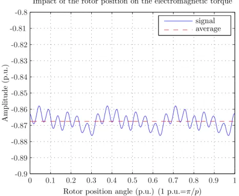
3.29 Impact of the rotor position on the electromagnetic torque . . . 72
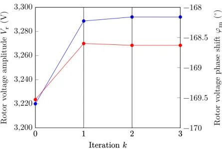
3.30 Evolution of rotor voltage during iteration process . . . 73
3.31 Control Structure for load operation . . . 76
3.32 Coupled FEM-Python simulation . . . 76
3.33 Controlled Simulation: Rotational speed . . . 77
3.34 Controlled Simulation: Electromagnetic torque . . . 78
3.35 Controlled Simulation: Rotor currents . . . 78
3.36 Controlled Simulation: Rotor currents in Park system . . . 79
3.37 Controlled Simulation: Stator currents . . . 79
3.38 Controlled Simulation: Stator currents in Park system . . . 80
4.1 Two-layer winding and coil opening . . . 83
4.2 Magneto-motive force created by one turn . . . 84
4.3 Magneto-motive-force distribution of each phase . . . 85
4.4 Magneto-motive-force spectrum of one phase . . . 86
4.6 Airgap permeance variation at one instant along two pole-pitches . . . 90
4.7 Single slot BEM model . . . 93
4.8 Single slot BEM results . . . 93
4.9 Double slotted airgap BEM model . . . 94
4.10 Double slotted airgap BEM results . . . 94
4.11 Permeance calculation model-position 1 . . . 95
4.12 Permeance calculation results-position 1 . . . 96
4.13 Permeance calculation model-position 2 . . . 96
4.14 Permeance calculation results-position 2 . . . 97
4.15 Multi-assembled reduced permeances . . . 97
4.16 Validation between the reduced and the complete models . . . 98
4.17 Airgap flux density at load without saturation . . . 100
4.18 Airgap flux density spectrum at load without saturation . . . 101
4.19 Saturated permeance . . . 102
4.20 Saturated permeance main coefficients . . . 102
4.21 Airgap flux density at no-load with saturation . . . 103
4.22 Airgap flux density spectrum at no-load with saturation . . . 104
4.23 Airgap flux density at load with saturation . . . 104
4.24 Airgap flux density spectrum at load with saturation . . . 105
4.25 Airgap transformation factor example . . . 106
4.26 Airgap flux density at load with saturation at the stator bore . . . 107
4.27 Airgap flux density at load with saturation at the rotor bore . . . 107
4.28 Simple magnetic network . . . 109
4.29 Permeance network: One slot pitch . . . 110
4.30 Permeance network: One pole pitch . . . 110
4.31 Simplified geometry for the BEM-Magnetic network calculation . . . 116
4.32 Boundary Element Method (BEM)-Magnetic network saturation state 1 . . . 116
4.33 BEM-Magnetic network saturation state 2 . . . 117
4.34 BEM-Magnetic network saturation state 3 . . . 117
4.35 BEM-FE comparison with a rough discretization . . . 118
4.36 BEM-FE comparison with a fine discretization . . . 119
4.37 BE model: Rough discretization . . . 119
4.38 BE model: Fine discretization . . . 120
5.1 FEM: Stator line-to-line voltage at rated no-load operation . . . 124
5.2 FEM: Stator line-to-line voltage spectrum at rated no-load operation . . . 125
5.3 THF weighting factors . . . 126
5.4 Voltage harmonic compatibility levels . . . 126
5.5 FEM: Effect of magnetization on slot harmonics . . . 127
5.6 FEM: Rotor phase current at rated no-load operation . . . 128
5.7 FEM: Effect of magnetization on slot harmonics . . . 128
5.9 Comparison analytical with BEM and FEM without saturation . . . 131
5.10 Comparison analytical with simple permeance formula and FEM without saturation131 5.11 Comparison analytical with BEM and FEM with saturation . . . 134
5.12 Impact of slip on rotor slot harmonics . . . 135
5.13 Impact of slip on THD (without converter harmonics) . . . 136
5.14 FEM: Coupling electrical circuit with simplified inverter . . . 136
5.15 FEM: Rotor voltages with simplified inverter . . . 137
5.16 FEM: Rotor currents with converter . . . 138
5.17 FEM: Stator voltages with converter . . . 138
5.18 FEM: Stator voltages spectrum with converter (without fundamental) . . . 139
5.19 Effect of the airgap length on the THD . . . 140
5.20 Effect of magnetic wedges on slot harmonics (zoom) . . . 141
5.21 Radial airgap magnetic flux vs time and airgap position . . . 145
5.22 Radial magnetic pressure vs time and airgap position . . . 145
5.23 Space and time harmonics of the radial magnetic pressure . . . 146
5.24 Model of the complete stator and frame . . . 146
5.25 2D FE model of the stator/frame system . . . 147
5.26 Examples stator structure eigen-modes . . . 147
5.27 Fundamental mode shape . . . 149
5.28 Vibration response . . . 154
5.29 Example of a fractional slot winding diagram . . . 156
5.30 Example of a fractional-slot winding diagram and mmf . . . 156
5.31 Stator mmf of the original winding . . . 158
5.32 Stator mmf spectrum of the original winding . . . 158
5.33 Stator mmf of the modified winding . . . 162
5.34 Stator mmf spectrum of the modified winding . . . 163
5.35 Effect of slip on force and vibration . . . 165
5.36 Effect of power factor on the vibration amplitude . . . 165
5.37 Machine M2: 2DFE geometry . . . 166
5.38 Force components 4-nodes, 100 Hz . . . 168
5.39 Evolution of vibration velocity va. power factor . . . 169
5.40 Induced fundamental voltage phasors . . . 170
5.41 Simple winding: fundamental winding coefficient evolution . . . 171
5.42 Iterative optimization results of the winding . . . 173
5.43 Iterative optimization results of the winding . . . 174
5.44 Iterative optimization results of the winding . . . 174
5.45 Iterative optimization results of the winding . . . 175
5.46 Iterative optimization results of the winding . . . 176
5.47 Iterative optimization results of the winding . . . 176
5.48 Iterative optimization results of the winding . . . 177
5.51 Iterative optimization results of the winding . . . 179
5.52 Electromagnetic torque for OP3 𝑠 = 0% . . . 182
5.53 Electromagnetic torque for OP1 𝑠 = −5% . . . 182
5.54 Shaft line as a three masses model . . . 188
5.55 Shaft line mode shapes . . . 189
5.56 Shaft line: angular position response . . . 191
5.57 Shaft line: torsion torque response . . . 192
5.58 Startup: Rotor current . . . 193
5.59 Startup: Stator current . . . 193
5.60 Startup: Mechanical speed . . . 194
5.61 Startup: Electromagnetic torque . . . 194
5.62 Startup: Electromagnetic torque (first instants) . . . 195
5.63 Sinusoidal flux density excitation . . . 198
5.64 Hysteresis cycles of typical stator and rotor materials . . . 198
5.65 Measured losses at 50 Hz for the material 𝑀 250 − 50𝐴 . . . 199
5.66 Measurement and model comparison for the material M250-50A at 50 Hz . . . . 200
5.67 Evolution of exponential coefficient 𝛼 for the material M250-50A . . . 200
5.68 Non-sinusoidal flux excitation . . . 201
5.69 Effect of non-sinusoidal flux excitation . . . 202
5.70 Identification of reversals . . . 202
5.71 Three types of excitation . . . 204
5.72 Elliptical excitation components . . . 204
5.73 Hysteresis loss correction factor . . . 206
5.74 Harmonic reduction factor due to slotting (example: 𝑝 = 7, 𝑁z= 294) . . . 207
5.75 Simnplified yoke geometry . . . 208
5.76 Magnetic flux density in the yoke (𝜈 = 𝑝,𝐵̂Y,𝜈= 1 T) . . . 209
5.77 Comparison of iron losses at no-load operation, hyper-synchronous mode . . . 211
5.78 Comparison of iron losses at load operation, hyper-synchronous mode . . . 212
5.79 Impact of magnetic wedges in iron losses under no-load operation . . . 213
6.1 Variation of mechanical and rotor active power v.s speed . . . 217
6.2 Total, copper and iron losses vs airgap depth . . . 220
6.3 Stator and rotor current density vs airgap depth . . . 221
6.4 Airgap flux density of the salient pole synchronous machine at no-load . . . 227
6.5 Airgap flux density of the double-fed induction machine at no-load . . . 228
6.6 Airgap flux density spectrum comparison at no-load . . . 228
6.7 Stator line-to-line voltages of the salient-pole synchronous machine at no-load . . 229
6.8 Stator line-to-line voltages of the double-fed induction machine at no-load . . . . 229
2.1 Machine characteristics for magnetic coefficients calculation . . . 23
3.1 Winding configuration example over two poles: 𝑞 = 3, 𝑌1= 7 . . . 45
3.2 Stator and rotor Leakage inductances elements . . . 50
3.3 Total Leakage inductances . . . 51
3.4 End-winding leakage inductance (Per Unit (p.u.)) . . . 53
3.5 Validation of a steady-state operation point . . . 80
3.6 Load points characteristics for validation . . . 80
4.1 Winding configuration example over two poles: 𝑞 = 4, 𝑌1= 10 . . . 84
4.2 Machine characteristics rotor and stator mmf calculation . . . 88
4.3 Machine characteristics for airgap permeance calculation . . . 99
4.4 Airgap permeance calculation result . . . 99
4.5 Geometry characteristics for the BEM-Magnetic network calculation . . . 115
5.1 Machine M1: load points characteristics . . . 148
5.2 Machine 𝑀1: design characteristics . . . 148
5.3 Machine M1: stator eigen-mode characteristics . . . 149
5.4 Machine 𝑀1: Calculated radial forces with analytical model . . . 150
5.5 Machine M1, OP1: Calculated radial forces with FE . . . 152
5.6 Machine M2: design characteristics . . . 157
5.7 Machine M2: load points characteristics . . . 157
5.8 Machine M2: Main electromagnetic forces . . . 159
5.9 Machine M2: stator eigen-mode characteristics . . . 160
5.10 Stator winding original configuration . . . 161
5.11 Stator winding new configuration . . . 162
5.12 Machine 𝑀2: Main electromagnetic forces for OP1, OP2and OP3with new winding164 5.13 Machine M2: Operation points for the FE study . . . 166
5.14 Characterization of the component 4-nodes, 100 Hz . . . 167
5.15 Load point characteristics for the electromagnetic torque computation . . . 181
5.16 Electromagnetic torque harmonics . . . 181
5.17 Inertia and stiffness coefficients . . . 189
5.18 Applied signals characteristics . . . 203
6.1 Example Machine Data 200-MVA Generator . . . 225
6.2 Optimization 1: variable input parameters and variation intervals . . . 225
6.3 Operation point for dimensioning . . . 226
6.4 Optimization 1 results: main input parameters . . . 226
6.5 Optimization 1 results: main output values . . . 227
6.6 Iron losses comparison at rated no-load operation (synchronous speed) . . . 230
6.7 Iron losses comparison at rated load operation (synchronous speed) . . . 231
6.8 Optimization 2: variable input parameters and variation intervals . . . 231
6.9 Optimization 2 results: main input parameters . . . 232
6.10 Optimization 2 results: main output values for the first design . . . 233
6.11 Iron losses comparison at rated load operation (hypo-synchronous speed) . . . . 233
2D Two-Dimensional
2DFE Two-Dimensional Finite Element 3D Three-Dimensional
3DFE Three-Dimensional Finite Element BDFIM Brushless Double-Fed Induction Machine
BE Boundary Element
BEM Boundary Element Method dc direct-current
DFIM Double-Fed Induction Machine FE Finite Element
FEM Finite Element method mmf magneto-motive force p.u. Per Unit
PSP Pumped-Storage Plants PWM Pulse Width Modulation RMS Root Mean Squared rpm Revolutions per minute
THD Telephone Harmonic Distortion THF Telephone Harmonic Factor VSI Voltage Switched Inverter
1.1 Regulating Power by using Pumped-Storage Hydro Power Plants
In order to respond to the increasing demand for electricity, more efficient solutions of energy production and storage have to be proposed.
Firstly, conventional sources of energy such as nuclear and gas power plants considered as the main Base-Load producers are able today to meet the principal demands of electricity. However such technologies are not able to respond quickly to sudden increases of energy demand. Solutions such as petrol or coal power plants are neither economical nor environmental-friendly. Secondly, the tendency motivated by environmental concerns is to offer alternative or com-plementary solutions to these main sources of energy. In this context wind power installation, for example, is continuously increasing as shown in Figure 1.1. Although renewable energies are viable technologies, the issue of sporadic availability, wind and solar not being constant, leads to problems for planning and regulation of power available on the network. In some cases the total supplied power might exceed the demand. This leads to a perturbation of the network frequency and can affect other elements connected to the network.
... .. 1996 . 1997 . 1998 . 1999 . 2000 . 2001 . 2002 . 2003 . 2004 . 2005 . 2006 . 2007 . 2008 . 2009 . 2010 . 2011 . 2012 . 0 . 50 . 100 . 150 . 200 . 250 . 300 . 6.1 . 7.6 . 10.2 . 13.6 . 17.4 . 23.9 . 31.1 . 39.4 . 47.6 . 59.1 . 73.9 . 93.9 . 120.6 . 158.9 . 198 . 238 . 282.6 . Gl obal Cum u lat iv e Inst all ed Wi nd Capaci ty (GW)
Figure 1.1: Global Cumulative Installed Wind Capacity 1996-2012 [GWE12]
Thirdly, electricity exchanges are today strongly governed by price and demand. This trading of energy leads to fluctuations of power and consequently instabilities of the network.
Hydro Pumped-Storage Plants (PSP) are used as network stabilizers and to achieve a balance between demand and supply. PSP are like any standard hydro power plant with motor/generator units coupled to hydro turbines. Such installations make it possible not only to deliver electricity
Maximum dam level
Maximum dam level
Minimum level
Minimum level Amount of exchanged water
Amount of exchanged water Minimum level
Minimum level
Maximum dam level
Maximum dam level
Figure 1.2: PSP structure [Sch06]
to the network but also to absorb power from the network. Electricity production is realized by providing water from an upper reservoir to a lower reservoir, mechanical power from the turbine is transformed into electricity via the motor/generator unit working as a generator. Electricity absorption is realized by pumping water from the lower reservoir to the upper reservoir. Elec-tricity in this case is transformed into stored potential energy via the motor/generator unit operating as a motor. Figure 1.2 provides an overview of a PSP structure.
In turbine operation, PSP makes it possible to fill the power gap when the demand is higher than the supply from the available energy sources. Alternately when the supply is higher than the demand, PSP in pumping operation stores the surplus energy.
Consequently PSP appears as an efficient means of energy storage and network power reg-ulation. PSP activity is continuously increasing which is directly linked to the expansion of renewable and nuclear energies, as shown in Figures 1.1 and 1.3. In order to improve the effi-ciency of PSP, variable-speed operation has been proposed. This is described in more detail in the next section.
1.2 Benefits of using Variable Speed for PSP applications
To dates conventional PSP installations have been mainly working at fixed speed. This means the turbine rotates at a fixed speed proportional to the network frequency. Such installations are equipped with a salient-pole synchronous motor/generator unit directly connected to the network via a transformer. Like standard synchronous machines, the stator consists of a three-phase winding carrying alternating current while the rotor is equipped with a simple winding, also called field winding, carrying a direct current. Figure 1.4 shows an example of such installation. Usually it is equipped with a reversible Francis-type runner, being able to work as a turbine in one direction and as a pump in the other direction. Note that, depending on the installation, generator and motor operations may also be done with a separate turbine and pump. This makes it possible to switch faster from the turbine to the pumping mode, but requires also more space than the reversible arrangement.
Figure 1.3: World wide expansion of PSP and nuclear activity [Sch+05]
In turbine operation, the active power is regulated by the opening and closing of the guide vanes. Regulation of the reactive power is done by controlling the field winding current. In motor operation the range of power variation is very limited. The only way to efficiently change the amount of power taken from the network is to change the speed of operation. For the past few years, variable-speed technology has been seriously studied as a relevant technology. With this technology it is possible to produce or absorb network power at constant frequency within a certain range of rotational speeds. In the following we describe the advantages of changing the speed of operation [SS97; Sch+05].
1.2.1 Better Control of the power in pumping mode
Pump characteristics are given as a function of Head (pressure) and Flow as shown in Figure 1.5. The operation point is obtained at the intersection between the actual head (on the graph H example) and the working speed. When considering a fixed speed, only one point exists (red circle). When the speed can be changed from 𝑁1 to 𝑁3, any operation points on the doted line can be reached. The blue circles are two accessible points and correspond to the minimum and maximum power. Depending on the head, the power can be varied over a range of thirty percent [Sch+05]. Changing the speed also makes it possible to work at the best efficiency given by the intersection (green circle) between the available head and the maximum efficiency line.
1.2.2 Work at the best operation point in turbine mode
Considering maximum and minimum operating head (𝐻max and 𝐻min) Francis-turbine design is normally optimized for pumping operation. As shown in Figure 1.6, the peak of the hill
Figure 1.4: Salient-pole synchronous motor/generator and turbine (Alstom image)
chart (in green), which is linked to the optimum operation, cannot be reached. Consequently the efficiency is limited during turbine operation. Changing the speed makes it possible to find other optimum working points for the turbine. Furthermore, the head, which is linked to the water level, is not a constant parameter over the time. The operation point of the turbine is changing and consequently the efficiency may decrease. Adjusting the speed makes it possible to work again at the best efficiency, over a range of available head.
Figure 1.7 compares, for a given installation, turbine relative efficiencies when considering fixed and variable-speed operation. In this case the relative increase of efficiency is about one percent with variable-speed operation.
1.2.3 Better tracking of the power
In turbine operation, PSP fixed-speed units only work when the demand of power is maximum, i.e. 100% of the unit-s rated power. Out of this zone, the machine is stopped. On the contrary variable-speed units make it possible to better follow the variation of the power. Consequently the power regulation is better and the number of starts/stops is reduced. Figure 1.8 highlights the possible zones of operation of both technologies and demonstrates the better tracking of the
Kavitation P max. Stability H example N 1 N synch. N 3 H min. H max. Flow H e a d η ηη ηmax.
Figure 1.5: Pump characteristics example [Sch+05]
Figure 1.7: Relative turbine efficiency for fixed and variable speed [Sch+05] power when using two variable-speed units compared to two fixed-speed units.
1.2.4 Better stabilization after a perturbation
In the case of DFIM machines (a specific type of variable-speed motor/generator unit which is described in Section 1.3.4) frequency, amplitude and phase shift of the rotor field can be regulated via an efficient control. Such machines re-stabilize the network faster after a perturbation than conventional generators. Figure 1.9 compares the behavior of fixed-speed and variable-speed units after a network voltage-drop perturbation.
1.3 Variable speed technologies
Given the theory of rotating magnetic fields [Cha80], stator and rotor magnetic fields must always rotate synchronously. This is expressed by:
𝑓s= 𝑓r+ 𝑓m (1.1)
where, 𝑓s is the stator frequency, 𝑓r is the rotor frequency and 𝑓m is the mechanical frequency. The mechanical frequency is related to the rotational speed 𝑛 expressed in Revolutions per minute (rpm),
𝑓m= 𝑛 ⋅ 𝑝
60 (1.2)
where 𝑝 is the number of pole pairs . When changing the speed i.e 𝑓m, 𝑓s or 𝑓rhas to be adapted. However, 𝑓s is set by the network and is constant and 𝑓r is equal to zero for fixed-speed units, as the current is direct-current1. Changing the rotational speed is consequently not possible
time 100 % 140 % 200 % 70 % time 100 % 140 % 200 % 70 % time 100 % 140 % 200 % 70 % time 100 % 140 % 200 % 70 % time 100 % 140 % 200 % 70 % time 100 % 140 % 200 % 70 % time 100 % 140 % 200 % 70 % time 100 % 140 % 200 % 70 %
Two fixed speed units
Two variable speed units
N e tw o rk p o w e r N e tw o rk p o w e r
Figure 1.8: Power tracking in turbine mode [Sch06]
0 speed [p.u.] 1 0.94 1 Time [s] 1 Time [s] speed [p.u.] 1 0.94 0
Figure 1.10: Dahlander couplings (left: 2 ⋅ 𝑝 pole-pairs), (right: 𝑝 pole-pairs), [Cha80] with a conventional installation and other technologies have to be proposed. There are several variable-speed technologies. Following is a review of the most common existing technologies.
1.3.1 The changeable/commutable salient-pole synchronous machine
For this configuration the rotor is supplied with direct-current (dc) current so that the rotor frequency is zero. Therefore the stator frequency is directly linked to the rotational speed by the relation:
𝑓s= 𝑛 ⋅ 𝑝
60 (1.3)
As the stator frequency is fixed by the network frequency, changing speed can only be done by changing the number of poles. The poles of a synchronous machine are connected in series, and the polarity is reversed between adjacent poles. By changing the connections, i.e. the polarities, different numbers of poles can be obtained. Figure 1.10 shows a simple change of connection in order to half the number of poles, and the corresponding airgap magnetic field. Finally two different numbers of poles are obtained and consequently two different speeds.
In hydraulic applications, identical or different rotor-pole shapes can be used. In order to reduce design complexity and keep acceptable performance (vibrations, losses) only two types of poles are chosen, and only two different number of poles are available. The first configuration in Figure 1.11, shows a ten-pole rotor with two different pole configurations, ten and height poles, and the corresponding airgap magnetic field. Changing connections modifies the distribution of the air-gap flux density and consequently affects the harmonic content. Using two different poles shape makes it possible to reduce the parasitic harmonics. In one case, all the poles are magnetized (second configuration), in the other case (third configuration) two poles are deactivated. The stator winding also needs to be modified. The number of stator poles must always be equal to the number of rotor poles. One solution is to install two independent stator windings, each with a different number of poles. Also, each stator phase could be separated into different sections and a different number of stator poles obtained by changing the connections [Xua76]. To operate as a pump, the machine needs to be started and taken to the operating speed. This can be done by several means: [Cha80; Can67]
sec-machine is taken to the operating speed by increasing gradually its turbine mechanical speed. The main machine accelerates in motor mode to the operational speed in synchro-nism with the secondary machine.
• Asynchronous start: Salient-pole synchronous machines are normally equipped with a damper-bar cage. This cage damps airgap harmonics responsible for losses and parasitic forces. It damps electromagnetic-torque oscillations and small speed variations. The damper winding can also be used for asynchronous start, but it needs to be designed specifically for this application.
• Variable frequency start: This is similar to back-to-back start, the difference being that the stator winding is supplied by a static frequency converter instead of the secondary machine. By increasing the stator frequency, the machine is progressively taken to synchronous speed.
Pole-changing technology gives the possibility to run at two different speeds. The disadvantages are clearly the complexity of the rotor and stator designs. One must also pay attention to the parasitic field harmonics created by the stator and rotor windings which lead to extra-losses on the stator, heating on the rotor surface and parasitic electromagnetic forces which cause noise and vibrations.
1.3.2 The salient-pole synchronous machine connected to a static converter
If the number of poles is constant, and supplied with dc current, modifying the rotor mechanical speed requires that the stator/terminal frequency be changed. However, the terminal frequency must equal the network frequency. In order to satisfy this rule, a frequency converter makes the interface between the machine and the network. An example of configuration is shown in Figure 1.12:
Such installations are mainly reserved for 50 MVA and smaller applications as the size and price of the converter depend on the exchanged power. When designing such machines, one must consider the current harmonics due to the converter. On the machine side these could lead to additional losses and electromagnetic forces causing vibrations and noise. On the grid side, these could result in pollution of the network, leading to additional losses in the transmission lines or perturbation of other connected elements (transformers, generators etc...). However such technology does not require any major design changes of the standard synchronous machine. Furthermore, technical improvement and cost decreases of power-electronic converter should lead to a rapid development of such technology.
1.3.3 The Brushless-Double-Fed Induction Machine
The main principle is to couple mechanically and electrically two induction machines by the rotor. One stator is connected to the network (power winding) and the other is connected to the network via a converter (command winding). This technology, also called tandem machine, requires a lot of place, and a condensed version using only one induction machine has been proposed.
(a) Commutable SP machines: Configuration 1
(b) Commutable SP machines: Configuration 2
(c) Commutable SP machines: Configuration 3
Field winding Terminal
Network
Converter
Figure 1.12: Salient poles synchronous machine with converter [Sch06]
The rotor has a squirrel-cage and the stator has two decoupled windings, one connected to the network (power winding) and one connected to the network via a converter (command winding). Brushless Double-Fed Induction Machine (BDFIM) is more and more debated in the literature. Liao [Lia96] presents the technology and compares this machine to the traditional squirrel-cage machine and makes from it a serious alternative to DFIM (see next section) for variable speed applications. Williamson [SFW97; SF97] presents the principles of modeling of the machine as well as design rules and explains how to choose the characteristics of the stator and rotor windings. Pozza [Poz+02] presents the principles of construction of an analytical model based on the extended model of the induction machine, details a control strategy and validates the model via measurements. Carlson [Car+06; McM+06] compares a BDFIM to a DFIM machine of same power. The losses are higher in the BDFIM. Although the rotor technology appears easier and cheaper than for the DFIM, the stator is more complex. This is due to the fact that two independent windings might have to share the same slots, which lead to higher slot dimensions, harmonics or insulation problems. Furthermore the efficiency of the machine might be lower due to the losses in the squirrel-cage rotor. One advantage of this technology is the absence of slip-rings which reduces periodic maintenance. Starting of the machine can be done by using the existing converter. The main disadvantage of the technology is the absence of industrial tests. For the moment such technology is limited to small power units such as small wind generators.
1.3.4 The Double-Fed Induction Machine
For this configuration, the stator is similar to that of a conventional synchronous machine and directly connected to the network. The rotor is equipped with a three-phase winding connected to the network via a converter. As opposed to the technology described in section 1.3.2, the converter of DFIM must only be designed for a fraction of the nominal power. This amount of power is directly linked to the admissible speed range of the machine, which is generally about ±10% of the synchronous speed. DFIM have been mainly used until now with cyclo-converters, as shown in Figure 1.13. Disadvantages of cyclo-converters are due to the fact that because of the use of thyristors the converter can only absorb reactive power and that the output frequency cannot be more than one third of the input frequency. This prevents the use of the converter for start-up in pump operation. An additional converter is therefore needed. Technical improvements of power electronics made possible a new generation of high-power converter Voltage Switched Inverter (VSI) as shown in Figure 1.14. Such technology corrects most of the disadvantages of cyclo-converter technology by enabling start, control of the reactive power on the rotor side, a strong reduction of parasitic current harmonics and a reduction of the needed installation volume (only one transformer for example).
Figure 1.13: DFIM with cyclo-converter [Sch+05]
Figure (1.15) and Figure (1.16) compare a conventional synchronous machine with a DFIM. One can observe the non-negligible place covered by the slip ring system in the case of the DFIM. Note that in the presented case, both machines present similar dimensions. However the DFIM will usually be larger than an equivalently rated salient-pole synchronous machine. More details about DFIM dimensioning are given in Chapter 6.
The main challenge of this technology is the complexity of the rotor due to mechanical and insulation issues as explained by the following points.
Figure 1.14: DFIM with VSI converter [Sch+05]
I. The rotor winding overhang
The rotor bars are similar to stator bars, one part installed in the core and the other part extending outside both ends of the core. In the core part, the bars are maintained in the slot by the slot wedges. Because of centrifugal forces during normal operation or worse in the case of over-speed, the overhang requires particular attention. Furthermore, in the case of faults such as short-circuits, the bars are subjected to very large forces. The overhang must always withstand such faults in order to avoid deformation or breaking. Several technologies exist to carry out this task, the most common being the use of glass tape epoxy to secure the overhang conductors. Although this solution is effective, it makes it difficult for maintenance operations such as inspection or replacement of bars. Another solution consists of using bolts [SV96].
II. The rotor bar insulation system
As described previously, the rotor is supplied by a frequency converter. Because of the Pulse Width Modulation (PWM) command, the output voltage contains high frequency (1 kHz) pulses. Depending on the impedance of the cable between the converter and the rotor terminals and of the rotor-winding, an over-voltage can appear at the rotor terminals. Furthermore, each pulse produces a high variation of voltage with time or high d𝑉 /d𝑡. These parasitic behaviors can lead to significant stresses of the winding insulation. Consequently the rotor bar insulation system must be designed to withstand these dielectric stresses.
III. Rotor lamination power losses
The rotor is composed of laminated steel which may be subjected to significant power losses. In synchronous operation, the main magnetic field in the rotor does not oscillate. The induced power losses in the lamination are essentially due to the harmonics created by the stator winding and by the airgap permeance harmonics and these losses are generally small. When not at synchronous speed, the rotor magnetic field is traveling with respect to the rotor. Therefore, in addition to the latter losses, other larger losses due to the flux varying at the slip frequency
(a) Double-Fed Induction Machine (b) Salient Pole Synchronous Machine
Figure 1.15: Cross section of the two machines (from Alstom design tool)
1000.0 996.0 1003.5 Ø 9966 Ø 5400 Ø 5854 997.8 1003.2
(a) Double-Fed Induction Machine
191.0 187.7 194.4 Ø 10000 Ø 5400 Ø 5900 Ø 7009 188.8 194.2
(b) Salient Pole Synchronous Machine
(𝑓s− 𝑓m) occur in the laminations. Normally, the lamination steel in the rotor is chosen to withstand the high mechanical stress. This choice cannot be done without a degradation of the material magnetic characteristics. Consequently the rotor lamination material has a larger specific loss than the stator lamination material. This must be considered when evaluating the losses and the cooling requirements of rotor.
IV. The rotor slip-ring and brushes
The slip-ring and carbon-brush systems are the interface between the converter and the three-phase winding of the rotor. The carbon-brush wear is strongly dependent on temperature and humidity and is subject to periodic maintenance.
1.3.5 Summary
Nevertheless knowledge acquired in the development of large conventional alternators i.e. 10 MVA to 800 MVA make it possible to overcome the previously listed difficulties. Large installations using DFIM have already been commissioned; the first one in 1987 by the Kansai Electric Power Company of Osaka Japan - a 18.5 MW motor-generator from Toshiba Corporation, then larger ones in 1993 (2×400 MW) from Hitachi were installed in Ohkawachi for commercial applications [Gre94; NK88]. Since then the interest for such technology has been growing gradually due to the major breakthrough in the power electronics. In 2003 one of the largest European hydro power plant (4 × 265 MW), Goldisthal, was commisioned. Two of the four generators are DFIM and provided by Siemens was commissioned. In 2015 and 2017 ALSTOM Renewable Power will put into operation the power plants at Linth Limmern (4 × 250 MW) and Nant de Drance (6 × 157 MW) in Switzerland using VSI converters.
1.4 Description and motivation of the study
1.4.1 Restriction of the study domainPrevious part described the actual solutions for developing motors/generator units able to run at variable speed. All these technologies present advantages and disadvantages. In order to select the most appropriate solutions for PSP applications, it is important to list the today required criteria:
• power of converter should be reduced in order to limit its size and its price • the output power is in the range 10 MVA to 500 MVA
• knowledge acquired in stator design of standard salient poles alternator should be appli-cable to the chosen machine
• a variation of ±10% of the reference speed should be accessible
Adjustable-pole machines can not be chosen because of the point 4. Although Synchronous machines with frequency converters satisfy the points 2, 3 and 4, the point 1 is not any more
respected when dealing with high output power alternators (more than 50 MVA). BDFIM and DFIM are the only machines able to respect the four rules. However BDFIM development remains today still limited and is mainly reserved for small power applications such as windmills. Furthermore DFIM has the advantage to have an identical stator to a conventional synchronous machine. This is particularly interesting during refurbishment of old PSP when considering the upgrade of a fixed-speed standard machine to a variable speed unit; in this case only the rotor needs to be changed. Finally the DFIM has been chosen and will be mainly analyzed in this thesis. The considered input/output power is in the range of 10 MVA to 500 MVA, the synchronous speed is in the range 200 rpm to 600 rpm.
1.4.2 Definition and motivation of the study
Motors/generators dedicated to hydraulic applications have long been studyied in the past. The available papers concern more particularly the synchronous machines and treat about their design and their optimization. The main analyzed subjects are the following:
• computation of equivalent circuit parameters [Can83; Ram03]
• Three-Dimensional Finite Element (3DFE) computation of end winding inductances and losses in the end regions [Tra03; Ric97; Sil94; ALP08]
• computation of iron losses [TA09; Ran+09] • computation of losses in the damper bars [TLS10]
• computation of radial electromagnetic forces [WK60; TLU12] • computation of stator voltage shape [KXS06; TSS03]
• computation of temperatures and cooling air-flow [TZS10]
Studies about the DFIM focus mainly on windmill generators and are often dedicated to control implementation and stability studies [Rob04; Pet05]. Regarding hydraulic applications the literature is also very rich in articles regarding control infrastructure and network studies. Schafer and Simond [SS97] compare the DFIM to the synchronous machine and show the bene-fits given in terms of network regulation and dynamic response. Hodder [Hod04] simulates the complete infrastructure of a hydraulic varspeed installation including the network and machine transformer and the converter. He shows the advantages of using a VSI instead of a cyclo-converter because of the lower harmonic distortion and the possibility to control the reactive power via the rotor. The control is based on a two-axis modeling of the machine and a de-coupling of the d and q axis in order to control the speed and the reactive power. Pannatier [Pan10] studies different control strategies and simulates the interaction of the machine with other components of the network such as thermal power plants or wind farms. He also presents a strategy to startup a DFIM and to synchronize it on the network. Besides control and stability topics, some studies [Lor97; Mil10] deal with the steady-state equations using the equivalent-scheme of the squirrel-cage induction motor in which a rotor voltage source is added. Lorenzen wrote several studies about the induction machine and the DFIM. In particular he worked on
iron-losses calculation [Lor96b] and describes with Herzog [LH93] the DFIM modeling principles. Witt [Wit98] worked also on the problem of the operation point determination considering the effect of saturation on the equivalent-circuit parameters. Furthermore Lorenzen wrote about the radial electromagnetic forces occurring in the DFIM [Lor09] and on the analytical determination of the stator core eigen-frequencies [Lor11]. The DFIM design tool used in Alstom is mainly based on the original tool DASM developed by Lorenzen. Muller-Feugga [Mul06] contributed to the validation of the design tool by carrying out 2DFE computations.
The object of this thesis is to review the principles of modeling and electromagnetic design of the DFIM dedicated to hydraulic applications.
Firstly, due to its topology, the design of DFIM requires special attention. Like any standard electrical machines, the total airgap magnetic field of a DFIM is the result of the interaction between stator and rotor magnetic fields. In addition to the main or working field, several para-sitic harmonics are superimposed. These harmonics are due to the distribution of the rotor and stator conductors in the slots. Furthermore the airgap of the DFIM is constant but modulated by the stator and rotor teeth which lead to extra harmonics called airgap permeance harmomics; this is even more crucial since the airgap of such machine is in general small. These harmonics are responsible in one hand for additional power losses on the stator and rotor magnetic core which must be considered when designing the cooling system of the machine. On the other hand, they create parasitic radial or tangential electromagnetic forces which by interacting with the stator or the shaft eigen-frequencies may create noise and vibration.
Secondly, due to fact that the speed can be varied the evaluation of the machine performance has to be done for the full range of speed. Change of speed leads to a shift of some of the rotor field harmonics frequencies. Consequently electromagnetic forces component frequencies can slip so that the risk to match an eigen-frequency from the stator or the shaft line becomes more important. Furthermore as explained in part 1.3.4, out of the synchronous speed, the rotor sees an alternating magnetic flux which is accountable for non negligible power losses.
Thirdly, the rotor winding of a DFIM is supplied with a VSI converter piloted by PWM command. Such command is generally responsible for extra harmonics in the rotor currents and consequently on the air gap field. It is important to quantify the effect of such modulation on the performance of the machine.
Finally, all these elements lead to the necessity to develop models to better understand the electromagnetic behavior of the DFIM. We will use for this the existing Alstom tool on which we propose improvements based on new modeling techniques and validations with Finite Element (FE) simulations. Such model will help to evaluate and finally to optimize the design of such machines.
1.4.3 Structure of the thesis
Chapter 2 presents the magnetic modeling of the DFIM based on a simple magnetic permeance network. The obtained simplified magnetic network is validated by carrying out 2DFE simula-tion. The developed model makes it possible to consider later the electromagnetic behavior on
the performance of the machine.
Chapter 3 defines an equivalent model of the machine for steady-state operation studies. Parameters of the model are obtained from analytical calculations based on the geometry of the machine. In particular the calculation of the stator and rotor leakage inductance is described according to the existing studies in the literature. 2DFE and 3DFE are used to validate the obtained results. The effect of magnetic saturation on the values of the circuit parameters is obtained by applying the results of the magnetic permeance model described in Chapter 2. Finally the load-point calculation is described and the results are validated by carrying out magneto-harmonic and time-stepping FE simulations. So as to efficiently perform these latter computations, an approach based on the regulation of the DFIM is described. It makes it possible to simulate any steady-state load conditions of the machine and also allows to either model the rotor power supply by standard sinusoidal voltage sources or by a simplified VSI. The developed method can be used to compute parasitic radial forces, dynamic torques or iron losses as it is shown in Chapter 5.
Chapter 4 deals with the problem of airgap flux density harmonics. Although Chapter 3 presents an accurate modeling of the DFIM, it considers that the airgap magnetic field varies sinusoidally. FE computations results have shown the necessity to complete this simplified approach by including additional harmonics such as the winding and the airgap permeance harmonics. The main originality is to use a modeling based on the BEM in order to consider efficiently the double-slotted airgap. The effect of saturation is included by applying a modula-tion of the airgap permeance based on the results of Chapter 3. This simplified approach makes it possible to deal with the saturation of the magnetic circuit on the main harmonics such as the fundamental wave and the third harmonic wave. However it does not make it possible to describe accurately its effect on other harmonics. A proposal for improvement for the future suggests to combine a simplified discretization of the stator and rotor cores using a magnetic permeance network and the accurate Boundary Element (BE) model of the air gap.
Chapter 5 uses the results of the previous chapters to study the behavior of different quantities such as the stator voltage harmonics, the radial electromagnetic forces, the dynamic electromag-netic torques and the iron losses. The developed algorithms are validated with FE simulations. We discuss in particular the impact of the saturation on the performance of the machine and the impact on the radial forces when using fractional slot windings. For the latter subject, we propose an original method (at the knowledge of the author) making it possible to optimize a winding in order to decrease the risk of vibration by exchanging some winding connections.
Chapter 6 reviews the design principles of the DFIM. Subjects such as the choice of rated parameters, the airgap length and the stator and rotor slots numbers are discussed. Furthermore it is shown how the dimensioning of the machine can be formulated as an optimization problem having some constraints and an objective function. In particular we study the transformation of an existing salient-pole synchronous machine into a DFIM changing first only the rotor then both the stator and the rotor. The method appears very efficient to find the main dimensions of the machine.
2.1 Introduction
Designing a rotating electrical machine requires the correct modeling of its magnetic circuit. The stator and rotor cores are made of magnetic iron sheets facing magnetic saturation. The magnetizing current which creates the magnetic flux is linked to the state of saturation so that a wrong assessment of the latter has a dramatic effect on the losses and consequently on the overall efficiency.
First part exposes a simplified analytical magnetic model of the DFIM based on the well-known Ampere-Maxwell theorem, applying a piecewise integration of the magnetic field strength along a chosen magnetic path. The magnetic potential drop calculation along the airgap as well as the different magnetic regions are described; a 2DFE calculation is used to accurately quantify the impact of the magnetic saturation on some design coefficients such as the pole enclosure coefficient and the airgap form factor. Finally the result of the magnetic integration makes it possible to compute the required magnetizing current in order to drive the magnetic flux through the magnetic circuit.
Second part compares the results of the magnetic circuit calculation obtained from the simpli-fied analytical magnetic model and from a 2DFE magneto-static computation. The comparison is made for various designs with regard to the magnetizing voltage and the stator and rotor teeth magnetic flux densities. This allows to certify the method for the full range of machines studied in this thesis.
2.2 The analytical magnetic model
2.2.1 The Ampere-Maxwell theoremThe chosen method is based on the application of the Ampere-Maxwell theorem. The integration of the magnetic field strength H over a closed path 𝒞 also called mmf 𝛩w is equal to the sum of all currents I crossing the domain enclosed by this path.
𝛩w(𝒞) = ∮ 𝒞
𝐻 ⋅ d𝑙 = ∑ 𝐼 (2.1)
Figure 2.1 shows a simplified illustration of the DFIM magnetic circuit as well as the integration path C chosen in order to cover one magnetic pole pitch.
1 pole pitch Stator yoke Rotor yoke Rotor tooth Stator tooth Airgap C
Θ
wFigure 2.1: Magnetic circuit
Five regions can be identified: the airgap, the stator teeth, the stator yoke, the rotor teeth and the rotor yoke. Except for the airgap region, the magnetic permeability of all regions depends on the magnetic material characteristics and on the crossing magnetic field strength. The integration of the magnetic field on the path 𝒞 consists of a piecewise integration of the magnetic strength on each identified region. Finally Equation (2.1) is expressed as Equation (2.2) where ̂𝑈m,ts, ̂𝑈m,ys, ̂𝑈m,tr and ̂𝑈m,δ are respectively the magnetic potential drops in the stator tooth, the stator yoke, the rotor tooth and the rotor yoke whereas 𝑈̂m,δ stands for the magnetic potential drop in the airgap.
𝛩w(𝒞) = ∮ 𝒞
𝐻 ⋅ d𝑙 = 2 ⋅ ̂𝑈m,ts+ ̂𝑈m,ys+ 2 ⋅ ̂𝑈m,tr+ ̂𝑈m,yr+ 2 ⋅ ̂𝑈m,δ (2.2)
2.2.2 The magnetizing voltage and flux
Only the rotor winding is supplied. The purpose is to calculate the rotor current in order to induce a certain voltage 𝑉s at the stator terminals. Note that at no-load 𝑉s is later equivalent to the magnetizing voltage 𝑉µ. 𝑉s can be obtained from the induction’s law:
𝑉s = −d𝛷f
where 𝛷f is the fundamental magnetizing flux. One can show that the airgap flux density contains several harmonic components inducing voltages on the stator winding1. However only the fundamental part of the flux density takes part in the effective power generation. The Root Mean Squared (RMS) value of the fundamental stator line-to-line voltage 𝑈rms
𝑠 is expressed as: 𝑈rms
𝑠 = √
3
2⋅ 2𝜋𝑓s⋅ 𝜉f,s𝑁s,s⋅ ̂𝛷f (2.4) where 𝜉f,sis the fundamental winding coefficient considering the winding configuration and 𝑁s,s is the number of stator winding turns in series. The maximum fundamental magnetic flux ̂𝛷f is obtained by integrating the fundamental airgap flux density 𝐵δ,f over the stator pole pitch 𝜏p,s so that: ̂ 𝛷f = 𝑙i∫ 𝜏p,s 0 ̂ 𝐵δ,f ⋅ sin(𝑥𝜋/𝜏p,s)d𝑥 = 2 𝜋𝑙s𝜏p,s⋅ ̂𝐵δ,f (2.5) where 𝑙i is the equivalent core length also called ideal length considering the presence of stator and rotor cooling air ducts2. Only the fundamental part of the magnetizing flux takes part in the effective power generation, however the magnetic state of the machine depends directly on the maximum value of the magnetizing flux 𝛷𝑚 expressed as:
̂
𝛷 = 𝑙i∫ 𝜏p,s
0
𝐵δ(𝑥) ⋅ d𝑥 = 𝑙s𝜏p,sαi⋅ ̂𝐵δ (2.6) where 𝐵δ(𝑥) describes the spatial evolution of the flux density along a path at the middle of the airgap, 𝐵̂δ is the maximum airgap flux density and αi is the so-called pole enclosure coefficient. Figure 2.2 shows the evolution of the airgap magnetic flux density 𝐵δ for three magnetizing currents (3/4 ⋅ 𝐼µ,0, 𝐼µ,0, 5/4𝐼µ,0) computed by FE. Note that 𝐼µ,0 corresponds to the magnetizing current under rated no-load operation. The spatial variation of 𝐵δ has been rebuilt in order to remove high order spatial harmonics due to the stator and rotor slots, furthermore for comparison purposes the evolution of the fundamental component 𝐵δ,f of the flux density is also displayed. One can see that the airgap flux density gets more and more flattened as the magnetizing current increases. Consequently αi depends on the magnetizing current and finally on the magnetic state of the machine.
Finally Equation (2.3) can be rewritten as a function of 𝛷, α̂ i and the form factor coefficient C1 = 𝐵̂δ,f/ ̂𝐵δ expressing the ratio between the fundamental airgap magnetic flux density and the maximum airgap magnetic flux density. One can identify an analogy with the salient-pole synchronous machine but in this case αi and 𝐶1 would mainly depend on the salient-pole geometry. 𝑈rms 𝑠 = √ 3 2 ⋅ 2𝜋𝑓s⋅ 𝜉f,s𝑁s,s⋅ 2 𝜋 ⋅ ̂𝛷 ⋅ C1 αi (2.7)
1See Chapter 4 for more details 2This ideal length 𝑙
Figure 2.2: Airgap flux density at different magnetizing states
2.2.3 The magnetic saturation coefficient
In order to quantify the magnetic state of the machine, the magnetic saturation coefficient Ks is defined as:
Ks = 2 ⋅ ̂𝑈m,ts+ ̂𝑈m,ys+ 2 ⋅ ̂𝑈m,tr+ ̂𝑈m,yr
2 ⋅ ̂𝑈m,δ (2.8)
When the magnetic circuit is not saturated, the magnetic drop in the iron regions is negligible compared to the magnetic drop in the airgap. Consequently Ks is equal to zero and as the airgap flux density contains mainly the fundamental component, the coefficients C1 and αi are respectively equal to one and 2/𝜋. When the magnetic circuit gets into saturation, the magnetic drop in the iron path is not any more negligible and the latter coefficients increase. The dependency law between the form coefficient C1 and the saturation coefficient Ks can be computed by carrying out a 2DFE simulation. By using a magneto-static resolution, where the magnetic field is constant, the rotor winding is supplied with a three-phase current system:
̂
𝐼r,a = 𝐼µ, 𝐼r,b̂ = −𝐼µ/2, 𝐼r,ĉ = −𝐼µ/2. The parameter 𝐼µ is varied in the range from 0.1 to 5.0 p.u., where 1 p.u. corresponds to the value of the rotor current under rated no-load operation. Note that in reality the excitation current will never reach such high values during no-load operation as the machine will get very saturated. For each value of 𝐼µ, the 2DFE simulation is solved. The flux density is computed over a path in the airgap and the values of the parameters 𝐵̂δ and 𝐵̂δ,f are extracted and with them the form factor coefficient C1. Furthermore, the saturation coefficient Ks is obtained by rewriting Equation (2.8) in Equation
Quantity min max
Apparent power 𝑆 (MVA) 150 400
Rated stator voltage 𝑈s (kV) 15 18
Stator bore diameter 𝐷b,s (mm) 4000 10000
Stator Core length 𝑙s (mm) 2000 4000
Minimum airgap length 𝛿𝑔 (mm) 14 18
Number of pole pairs 𝑝 (-) 6 8
Number of stator slots per pole/phase 𝑞s (-) 4 8 Number of rotor slots per pole/phase 𝑞r (-) 3 7 Stator yoke height/stator yoke pole pitch ℎy,s/τy,s(-) 0.20 0.35 Rotor yoke height/rotor yoke pole pitch ℎy,r/τy,r (-) 0.45 1.05 Stator tooth width/stator slot pitch 𝑤t,s/τ𝑠,s (-) 0.3 0.5 Rotor tooth width/rotor slot pitch 𝑤t,r/τ𝑠,r (-) 0.25 0.4 Table 2.1: Machine characteristics for magnetic coefficients calculation (2.9) by considering Equation (2.2)
Ks=
̂
𝛩w(𝒞) − 2 ⋅ ̂𝑈m,δ
2 ⋅ ̂𝑈m,δ (2.9)
where 𝛩̂w(𝒞) is the total mmf created by the rotor currents and 𝑈̂m,δ is the magnetic drop in the airgap described further in this part by Equation (2.12). 𝛩̂w(𝒞) can be obtained from Equation (2.10) where 𝜃 represents the magnetic voltage created by the rotor currents, the scaling coefficient 2 comes from the fact that both pole positive and negative are crossed by the magnetic field. In the case of a three-phase winding and by considering only the fundamental component, ̂𝜃 is obtained from Equation (2.11)3.
̂ 𝛩w(𝒞) = 2 ⋅ ̂𝜃 (2.10) ̂ 𝜃 ≈ 6 √ 2 𝜋 ⋅ 𝑁s,r𝜉f,r 𝑝 ⋅ 𝐼 rms r (2.11)
where 𝑁s,r is the number of rotor series turns, 𝜉f,r is the fundamental rotor winding coefficient and 𝐼rms
r is the RMS value of the current in the rotor winding; here 𝐼rrms = 𝐼µ̂ / √
2. These calculations are made for a wide range of machine designs provided in Table 2.1.
Figure 2.3 and Figure 2.4 show the corresponding variations of the coefficients C1 and αi. There is a slight change in the variation of C1 and αi from one design to another. However one can also identify a common trend as shown by the red line on both graphs. Note that during rated no-load or load operation Ks ∈ [0.2 ⋯ 0.4].
Finally for a given value of the fundamental magnetizing voltage, one can express the cor-responding maximum magnetic flux. The corcor-responding magnetic drops in all the sections previously defined can be computed as demonstrated in the next part.
Figure 2.3: Form factor C1