Real-time multimodal semantic scene understanding for autonomous UGV navigation

HAL Id: tel-03154783

https://tel.archives-ouvertes.fr/tel-03154783

Submitted on 1 Mar 2021

HAL is a multi-disciplinary open access archive for the deposit and dissemination of sci-entific research documents, whether they are pub-lished or not. The documents may come from teaching and research institutions in France or abroad, or from public or private research centers.

L’archive ouverte pluridisciplinaire HAL, est destinée au dépôt et à la diffusion de documents scientifiques de niveau recherche, publiés ou non, émanant des établissements d’enseignement et de recherche français ou étrangers, des laboratoires publics ou privés.

Yifei Zhang

To cite this version:

Yifei Zhang. Real-time multimodal semantic scene understanding for autonomous UGV naviga-tion. Image Processing [eess.IV]. Université Bourgogne Franche-Comté, 2021. English. �NNT : 2021UBFCK002�. �tel-03154783�

TH `ESE DE DOCTORAT

DE L’ ´ETABLISSEMENT UNIVERSIT ´E BOURGOGNE FRANCHE-COMT ´E

PR ´EPAR ´EE `A L’UNIVERSIT ´E DE BOURGOGNE

´

Ecole doctorale n°37

Sciences Pour l’Ing ´enieur et Microtechniques

Doctorat d’Instrumentation et informatique d’image

par

YIFEI

ZHANG

Real-time multimodal semantic scene understanding for autonomous

navigation

Th `ese pr ´esent ´ee et soutenue `a Le creusot, le 19 January 2021 Composition du Jury :

FREMONT VINCENT Professeur `a Ecole Centrale Nantes Rapporteur

AINOUZ SAMIA Professeur `a INSA Rouen Rapporteur

DUCOTTET CHRISTOPHE Professeur `a Universit ´e St-Etienne Examinateur/Pr ´esident

MOREL OLIVIER MCF `a Univ. de Bourgogne Franche-Comt ´e Co-encadrant

M ´ERIAUDEAU FABRICE Professeur `a Univ. de Bourgogne

Franche-Comt ´e

Co-directeur de th `ese

SIDIBE D ´´ ESIRE´ Professeur `a Universit ´e Paris-Saclay Co-directeur de th `ese

A

CKNOWLEDGEMENTS

First of all, I would like to express my sincere gratitude to my supervisors D ´esir ´e Sidib ´e, Olivier Morel, and Fabrice M ´eriaudeau for their constant encouragement and guidance on my thesis. Without their patient instruction, insightful criticism, and expert guidance, the completion of experiments and papers would not have been possible. In preparing the doctoral thesis, they have spent much time reading through each draft and provided me with inspiring advice. I am very thankful to D ´esir ´e for his continuous support and valuable advice in all our discussions. Thank him for choosing me and giving me the chance to pursue my dream of scientific research. I am very grateful to Olivier for his insightful comments, which enable my thesis work further improved, and thanks for his encouragement, which makes me more confident in my presentation. I would also like to convey my sincere thanks to Fabrice for his patience, motivation, enthusiasm, and trust.

Then, my faithful appreciation also goes to the jury members for their kindness in par-ticipating in my Ph.D. defense committee. Many thanks to Prof. Vincent Fremont and Prof. Samia Ainouz for their precious time reading the thesis and their constructive re-marks, and to Prof.Christophe Ducottet for his support as the president of the defense and valuable suggestions for the thesis work.

I also owe my sincere gratitude to Samia B. and Frederick for their friendly reception. During my visit to the IBISC laboratory, they have provided a lot of convenience for my life and work. During the epidemic, they provided me with the necessary conditions to prevent epidemics and tried their best to ensure my health and research progress.

I would also like to thank all my colleagues in the VIBOT team. During the two years in Le Creusot, they have given me generous support and kindness in my research work and teaching. To name a few: David F., C ´edric, Ralph, Nathalie, Christophe S., Christophe L., Zawawi, Nathan P., Thomas, Thibault, Daniel... I am incredibly very thankful to Mo-jdeh and Cansen for their help in my early work of the thesis. They spent a lot of time teaching me how to do academic research and developing good research habits. Be-sides, I enjoyed the time working with Marc. I have fond memories of the days when we went to Prague to attend the conference. I also miss having dinner with friends and play-ing games at Mojdeh and Guillaume’s house, climbplay-ing with David S., eatplay-ing Girls’ lunch with Ashvaany and Abir, training with Raphael and Nathan C. in Toulouse, with Eric and Fauvet taught in Nanjing together... Thank you very much for giving me many precious memories. Although I am far away from home, I still feel warm because of them.

Last, my thanks would go to my beloved family for their loving considerations and great confidence in me all through these years. Also, I would like to express my love to my boyfriend Qifa, who gave me endless tenderness and time in listening to me and help me fight through the tough times. Their love and support make my dream come true.

C

ONTENTS

1 Introduction 1

1.1 Context and Motivation . . . 1

1.2 Background and Challenges . . . 3

1.2.1 Multimodal Scene Understanding . . . 3

1.2.2 Semantic Image Segmentation . . . 4

1.2.3 Deep Multimodal Semantic Segmentation . . . 5

1.2.4 Scenarios and Applications . . . 7

1.2.5 Few-shot Semantic Segmentation . . . 7

1.3 Contributions . . . 8

1.4 Organization . . . 9

2 Background on Neural Networks 11 2.1 Basic Concepts . . . 12

2.1.1 Convolution . . . 12

2.1.2 Convolutional Neural Networks . . . 13

2.1.3 Encoder-decoder Architecture . . . 14

2.2 Neural Network Layers . . . 15

2.2.1 Convolution layer . . . 15

2.2.2 Pooling Layer . . . 16

2.2.3 ReLu Layer . . . 17

2.2.4 Fully Connected Layer . . . 17

2.3 Optimization . . . 18

2.3.1 Batch Normalization . . . 18

2.3.2 Dropout . . . 18

2.4 Model Training . . . 19

2.4.1 Data Preprocessing . . . 19 2.4.2 Weight Initialization . . . 20 2.4.3 Loss Function . . . 20 2.4.4 Gradient Descent . . . 22 2.5 Evaluation Metrics . . . 23 2.6 Summary . . . 24 3 Literature Review 25 3.1 Fully-supervised Semantic Image Segmentation . . . 26

3.1.1 Taxonomy of Deep Multimodal Fusion . . . 26

3.1.1.1 Early Fusion . . . 27 3.1.1.2 Late Fusion . . . 28 3.1.1.3 Hybrid Fusion . . . 29 3.1.1.4 Statistical Fusion . . . 31 3.1.2 Discussion . . . 32 3.2 Datasets . . . 34

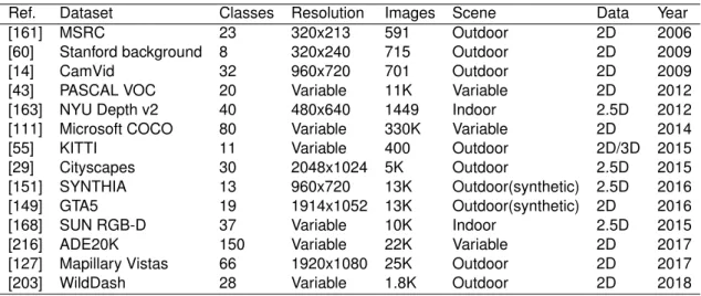
3.2.1 Popular Datasets for Image Segmentation Task . . . 34

3.2.2 Multimodal Datasets . . . 36

3.2.2.1 RGB-D Datasets . . . 36

3.2.2.2 Near-InfraRed Datasets . . . 37

3.2.2.3 Thermal Datasets . . . 38

3.2.2.4 Polarization Datasets . . . 38

3.2.2.5 Critical Challenges for Multimodal Data . . . 39

3.2.3 Comparative Analysis . . . 40

3.2.3.1 Accuracy . . . 40

3.2.3.2 Execution Time . . . 43

3.2.3.3 Memory Usage . . . 44

3.3 Summary . . . 44

4 Deep Multimodal Fusion for Semantic Image Segmentation 47 4.1 CMNet: Deep Multimodal Fusion for Road Scene Segmentation . . . 48

CONTENTS vii 4.1.1 Introduction . . . 48 4.1.2 Baseline Architectures . . . 49 4.1.2.1 Early Fusion . . . 49 4.1.2.2 Late Fusion . . . 50 4.1.3 Proposed Method . . . 50 4.1.4 Dataset . . . 52 4.1.4.1 Polarization Formalism . . . 52 4.1.4.2 POLABOT Dataset . . . 54 4.1.5 Experiments . . . 55

4.1.5.1 Evaluation on Freiburg Forest Dataset . . . 55

4.1.5.2 Evaluation on POLABOT Dataset . . . 58

4.2 A Central Multimodal Fusion Framework . . . 59

4.2.1 Introduction . . . 59

4.2.2 Method . . . 60

4.2.2.1 Central Fusion . . . 60

4.2.2.2 Adaptive Central Fusion Network . . . 60

4.2.2.3 Statistical Prior Fusion . . . 61

4.2.3 Experiments . . . 63

4.2.3.1 Implementation Details . . . 63

4.2.3.2 Evaluation on POLABOT Dataset . . . 64

4.2.3.3 Evaluation on Cityscapes Dataset . . . 64

4.3 Summary . . . 67

5 Few-shot Semantic Image Segmentation 69 5.1 Introduction on Few-shot Segmentation . . . 70

5.2 MAPnet: A Multiscale Attention-Based Prototypical Network . . . 70

5.2.1 Introduction . . . 70

5.2.2 Problem Setting . . . 72

5.2.3 Method . . . 72

5.2.4.1 Setup . . . 74

5.2.4.2 Evaluation . . . 75

5.2.4.3 Test with weak annotations . . . 76

5.3 RDNet: Incorporating Depth Information into Few-shot Segmentation . . . . 78

5.3.1 Introduction . . . 78 5.3.2 Problem Setting . . . 80 5.3.3 Method . . . 81 5.3.4 Cityscapes-3i Dataset . . . 83 5.3.5 Experiments . . . 84 5.3.5.1 Setup . . . 84 5.3.5.2 Experimental Results . . . 84 5.3.5.3 Feature Visualization . . . 86 5.4 Summary . . . 86

6 Conclusion and Future Work 89 6.1 General Conclusion . . . 89

L

IST OF

F

IGURES

1.1 Example of multimodal semantic segmentation from Cityscapes dataset.

The prediction was generated by our CMFnet+BF2 framework. . . 2

1.2 Number of papers published per year. Statistical analysis is based on the work by Caesar [15]. Segmentation includes image/instance/panoptic seg-mentation and joint depth estimation. . . 4

1.3 An illustration of deep multimodal segmentation pipeline. . . 5

2.1 Example of a convolutional neural network with four inputs. . . 13

2.2 Example of the encoder-decoder architecture. . . 15

2.3 Example of max pooling operation. . . 16

2.4 Examples of popular activation functions. . . 17

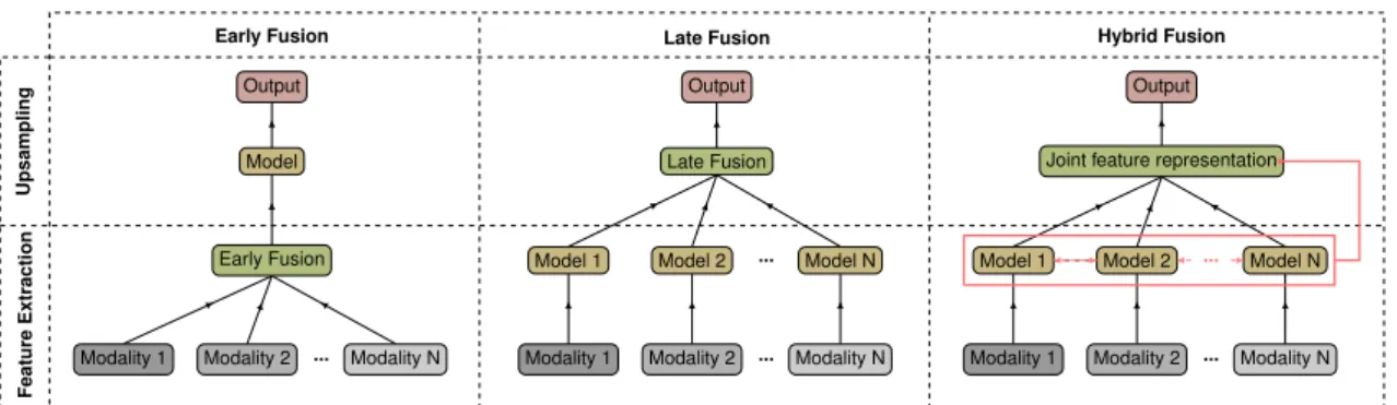
3.1 An illustration of different fusion strategies for deep multimodal learning. . . 26

3.2 FuseNet architecture with RGB-D input. Figure reproduced from [69]. . . . 28

3.3 Convoluted Mixture of Deep Experts framework. Figure extracted from [177]. 29 3.4 Fusion architecture with self-supervised model sdaptation modules. Figure extracted from [177]. . . 30

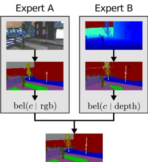
3.5 Individual semantic segmentation experts are combined modularly using different statistical methods. Figure extracted from [13] . . . 31

3.6 Accumulated dataset importance. Statistical analysis is based on the work by [15]. . . 33

3.7 Real-time and accuracy performance. Performance of SSMA fusion method using different real-time backbones on the Cityscapes validation set (input image size: 768 × 384, GPU: NVIDIA TITAN X). . . 43

3.8 Real-time and accuracy performance. Performance of different fusion methods on the Tokyo Multi-Spectral dataset.(input image size: 640 × 480, GPU: NVIDIA 1080 Ti graphics card). . . 44

4.1 Typical early fusion and Late fusion architectures comparison. . . 49

4.2 Our proposed fusion architecture: CMnet for multimodal fusion based on late fusion architecture. . . 51

4.3 The electric and magnetic field of light as well as their continuous self-propagating. . . 53

4.4 Reflection influence on polarimetry. (a) and (b) represent a zoom on the non-polarized and polarized area, respectively. Figure extracted from [11]. . 54

4.5 (a) Mobile robot platform used for the acquisition of the POLABOT dataset. It is equipped with the IDS Ucam, PolarCam, Kinect 2 and a NIR camera. (b)(c)(d) Multimodal images in the POLABOT dataset. . . 55

4.6 Two segmented examples from Freiburg Forest dataset. RGB and/or EVI images were given as inputs. . . 57

4.7 Two segmented examples from POLABOT dataset. RGB and/or POLA images were given as inputs. . . 58

4.8 Typical fusion strategies with RGB and depth input. (a) Early fusion. (b) Late fusion. (c) Central fusion. As a comparison, the proposed fusion structure integrates the feature maps in a succession of layers into a central branch. . . 60

4.9 Overview of the central fusion network (CMFnet). The adaptive gating unit automatically produces the weights of modality-specific branch in each layer. GAP denotes to Global Average Pooling, ”x” means multiplication, ”C” means concatenation. . . 62

4.10 Training loss of models on the POLABOT dataset. . . 65

4.11 Improvement/error maps of the proposed CMFnet and CMFnet+BF2 in comparison to the RGB baseline. Note that the improved pixels and the misclassified pixels are recorded in green and red, respectively. . . 66

4.12 Segmentation results on the POLABOT dataset. The first row of examples contains the RGB image and the corresponding polarimetric image. The second row of examples shows, from left to right, the ground truth image, the segmentation outputs of the individual experts (RGB and Polar), and the fusion results of CMFnet-BF2 and CMFnet-BF3. . . 67

4.13 Two sets of segmentation results on Cityscapes dataset. The first row of examples contains the RGB image and the corresponding depth image. From left to right of the second row of examples: ground truth, the pre-diction of RGB input, average and LFC. From left to right of the second row of examples: the fusion results of CMoDE, CMFnet, CMFnet-BF2 and CMFnet-BF3, respectively. . . 68

LIST OF FIGURES xi

5.1 An overview of the proposed method (MAPnet). Given a query image of a new category, e.g., aeroplane, the goal of few-shot segmentation is to predict a mask of this category regarding only a few labeled samples. . . . 71

5.2 Illustration of the proposed method (MAPnet) for few-shot semantic seg-mentation. . . 73

5.3 Qualitative results of our method for 1-way 1-shot segmentation on the PASCAL-5i _{dataset. . . . 77}

5.4 Training loss of models with and without attention-based gating (ABG) for 1-way 1-shot segmentation on PASCAL-50_{. . . 78}

5.5 Qualitative results of our model using scribble and bounding box anno-tations for 1-way 5-shot setting. The chosen example in support images shows the annotation types. . . 79

5.6 Overview of the proposed RDNet approach. R and D indicate the RGB and depth image input, respectively. The abstract features of labeled sup-port images are mapped into the corresponding embedding space (cir-cles). Multiple prototypes (blue and yellow solid circles) are generated to perform semantic guidance (dashed lines) on the corresponding query fea-tures (rhombus). RDNet further produces the final prediction by combining the probability maps from RGB and depth stream. . . 80

5.7 Details of the proposed RDNet architecture. It includes two mirrored streams: an RGB stream and a depth stream. Each stream processes the corresponding input data, including a support set and a query set. The prototypes of support images are obtained by masked average pooling. Then the semantic guidance is performed on the query feature by comput-ing the relative cosine distance. The results from these two streams are combined at the late stage. . . 82

5.8 Qualitative results of our method for 1-way 1-shot semantic segmentation on Cityscapes-3i_{. . . 86}

5.9 Visualization using t-SNE [179] for RGB and depth prototype representa-tions in our RDNet. . . 87

L

IST OF

T

ABLES

3.1 Typical early fusion methods reviewed in this chapter. . . 27

3.2 Typical late fusion methods reviewed in this chapter. . . 29

3.3 Typical hybrid fusion methods reviewed in this chapter. . . 30

3.4 Summary of popular datasets for image segmentation task. . . 35

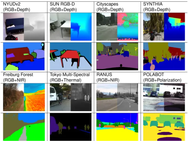
3.5 Summary of popular 2D/2.5D multimodal datasets for scene understanding. 36 3.6 Examples of multimodal image datasets mentioned in Subsection 3.2.2. For each dataset, the top image shows two modal representations of the same scene. The bottom image is the corresponding groundtruth. . . 39

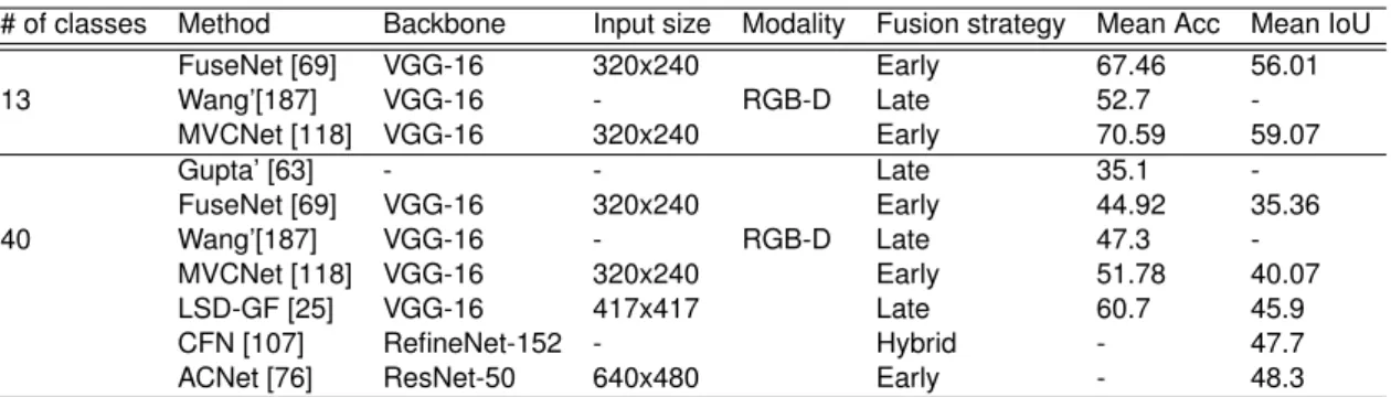
3.7 Performance results of deep multimodal fusion methods on SUN RGB-D dataset. . . 40

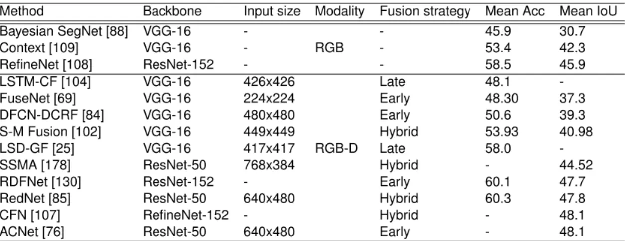
3.8 Performance results of deep multimodal fusion methods on NYU Depth v2 dataset. . . 41

3.9 Experimental results of deep multimodal fusion methods on Cityscapes dataset. Input images are uniformly resized to 768 × 384. . . 41

3.10 Experimental results of deep multimodal fusion methods on Tokyo Multi-Spectral dataset. The image resolution in the dataset is 640 × 480. . . 42

3.11 Parameters and inference time performance. The reported results on the Cityscapes dataset are collected from [178]. . . 44

4.1 Performance of segmentation models on Freiburg Multispectral Forest dataset. EF, LF refer to early fusion and late fusion respectively. We report pixel accuracy (PA), mean accuracy (MA), mean intersection over union (MIoU), frequency weighted IoU (FWIoU) as metric to evaluate the perfor-mance. . . 56

4.2 Comparison of deep unimodal and multimodal fusion approaches by class. We report MIoU as metric to evaluate the performance. . . 56

4.3 Segmentation performance on POLABOT dataset . . . 59

4.4 Performance comparison of our method with baseline models on the PO-LABOT dataset. Note that SegNet is used as the unimodal baseline and the backbone of multimodal fusion methods. . . 65

4.5 Ablation study of our method. Per class performance of our proposed framework in comparison to individual modalities with ENet baseline on Cityscapes dataset. . . 66

4.6 Performance of fusion models with ENet backbone on Cityscapes dataset. 66

5.1 Training and evaluation on PASCAL-5i _{dataset using 4-fold}

cross-validation, where i denotes the number of subsets. . . 75

5.2 Results of 1-way 1-shot and 1-way 5-shot semantic segmentation on PASCAL-5i using mean-IoU(%) metric. The results of 1-NN and LogReg are reported by [158]. . . 76

5.3 Results of 1-way 1-shot and 1-way 5-shot segmentation on PASCAL-5i

us-ing binary-IoU(%) metric. ∆ denotes the difference between 1-shot and 5-shot. . . 76

5.4 Evaluation results of using different types of annotations in mean-IoU(%) metric. . . 78

5.5 Training and evaluation on Cityscapes-3i _{dataset using 3-fold}

cross-validation, where i denotes the number of subsets. . . 83

5.6 Results of 1-way 1-shot and 1-way 2-shot semantic segmentation on Cityscapes-5i using mean-IoU(%) metric. . . 85

5.7 Per-class mean-IoU(%) comparison of ablation studies for 1-way 1-shot semantic segmentation . . . 85

5.8 Results of 1-way 1-shot semantic segmentation using binary IoU and the runtime. . . 86

1

I

NTRODUCTION

1.1/

C

ONTEXT AND

M

OTIVATION

Since the 1960s, scientists are dedicated to creating machines that can see and under-stand the world like humans, which led to the emergence of computer vision. It has now become an active subfield of artificial intelligence and computer science for processing visual data. This thesis tackles the challenge of semantic segmentation in scene under-standing, particularly multimodal image segmentation of the outdoor road scenes. Se-mantic segmentation, as a high-level task in the computer vision field, paves the way towards complete scene understanding. From a more technical perspective, seman-tic image segmentation refers to the task of assigning a semanseman-tic label to each pixel in the image [129, 54, 202]. This terminology was further distinguished from instance-level segmentation [38] that devotes to produce per-instance mask and class label. Recently, panoptic segmentation [91, 24] is getting popular which combines pixel-level and instance-level semantic segmentation. Although there are many traditional machine learning algorithms available to tackle these challenges, the rise of deep learning tech-niques [96, 59] gains unprecedented success and tops other approaches by a large mar-gin. The various milestones in the evolution of deep learning significantly promote the advancement of semantic segmentation research.

Especially in recent years, deep multimodal fusion methods benefit from the massive amount of data and increased computing power. These fusion methods fully exploit hierarchical feature representations in an end-to-end manner. Multimodal information sources provide rich but redundant scene information, which also accompanied by un-certainty. Researchers engage in designing compact neural networks to extract valuable features, thus enhancing the perception of intelligent systems. The underlying motivation for deep multimodal image segmentation is to learn the optimal joint representation from rich and complementary features of the same scene. Moreover, the availability of multiple sensing modalities has encouraged the development of multimodal fusion, such as 3D LiDARs, RGB-D cameras, thermal cameras, etc. These modalities are usually used as

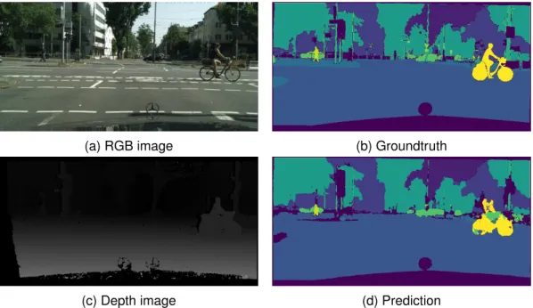
(a) RGB image (b) Groundtruth

(c) Depth image (d) Prediction

Figure 1.1: Example of multimodal semantic segmentation from Cityscapes dataset. The prediction was generated by our CMFnet+BF2 framework.

complementary sensors in complex scenarios, reducing the uncertainty of scene informa-tion. For example, visual cameras perform advanced information processing in lighting conditions, while LiDARs are robust to challenging weather conditions such as rain, snow, or fog. Thermal cameras work well in the nighttime as they are more sensitive to infrared radiation emitted by all objects with a temperature above absolute zero [50]. Arguably, the captured multimodal data provide more spatial and contextual information for robust and accurate scene understanding. Compared to using a single modality, multi-modalities significantly improve the performance of learning models [40, 113, 197, 2, 199]. Figure 1.1 illustrates an example of semantic image segmentation with RGB and depth input.

Besides, much research dedicates to exploring advanced technologies under limited su-pervision. Recently, few-shot learning has emerged as a hot topic in the computer vision community. Deep learning-based image understanding techniques require a large num-ber of labeled images for training. Few-shot semantic segmentation, on the contrary, aims at generalizing the segmentation ability of the model to new categories given a few sam-ples. Namely, the trained neural network predicts pixel-level mask of new categories on the query image, given only a few labeled support images. In this thesis, we explore the attention mechanism-based method for few-shot segmentation task, aiming to improve the semantic feature representation and generalization capabilities of the models.

However, the generalization and discrimination abilities of existing unimodal few-shot seg-mentation methods still remain to be improved, especially for complex scenes. The semantic understanding of outdoor road scenes is usually affected by environmental changes, such as occlusion of objects and variable lighting conditions, which makes

1.2. BACKGROUND AND CHALLENGES 3

learning and prediction of the few-shot network difficult. In order to obtain complete scene information, we are also committed to extending the RGB-centric approach to take ad-vantage of complementary depth information. The original intention of our work is to incorporate supplementary multimodal image information into a few-shot segmentation model. These multimodal data provide rich color and geometric information of scenes, leading to more accurate segmentation performance.

1.2/

B

ACKGROUND AND

C

HALLENGES 1.2.1/ MULTIMODAL SCENEUNDERSTANDING

Humans live in a complex multi-source environment. Whether it is video, image, text or voice, each form of information can be called a modality. We adopt the definition of modal-ityfrom [95], which refers to each detector acquiring information about the same scene. The range of modalities is wider than our perception ability. In addition to the information obtained by vision, we can also collect multimodal information by various sensors such as radar and infrared cameras. Multimodal fusion systems work like the human brain, which synthesizes multiple sources of information for semantic perception and further decision making. Ideally, we would like to have an all-in-one sensor to capture all the informa-tion, but for most complex scenarios, it is hard for a single modality to provide complete knowledge. Consequently, the primary motivation for multimodal scene understanding is to obtain rich characteristics of the scenes by integrating multiple sensory modalities. Our work focuses on deep learning-based multimodal fusion technology, which also in-volves multimodal collaborative learning, multimodal feature representation, multimodal alignment, etc.

As a multi-disciplinary research, the meaning of multi-modality varies in different fields. For example, in medical image analysis, the principal modalities involve Computed To-mography (CT), Magnetic Resonance Imaging (MRI), Positron Emission ToTo-mography (PET), Single-Photon Emission Computed Tomography (SPECT) [112], to name a few. Benefiting from the complementary and functional information about a target (e.g., organ), multimodal fusion models can achieve a precise diagnosis and treatment [122, 116, 217]. In multimedia analysis, multimodal data collected from audio, video as well as text modal-ities [3, 126, 6] are used to tackle semantic concept detection, including human-vehicle interaction [41], biometric identification [49, 167, 28]. In remote sensing applications, mul-timodal fusion leverages the high-resolution optical data, synthetic aperture radar, and 3D point cloud [4, 206]. In this thesis, we clarify the definition ofmodalityfor semantic seg-mentation tasks as a single image sensor. Relevant sensory modalities reviewed and experimented include RGB-D cameras, Near-InfraRed cameras, thermal cameras, and

2010201120122013201420152016201720182019 0 50 100 150 Year N umber o f pa per s Segmentation

Figure 1.2: Number of papers published per year. Statistical analysis is based on the work by Caesar [15]. Segmentation includes image/instance/panoptic segmentation and joint depth estimation.

polarization cameras.

1.2.2/ SEMANTIC IMAGE SEGMENTATION

In recent years, there have been many studies addressing semantic image segmentation with deep learning techniques [54, 56]. As a core problem of computer vision, scene understanding relies heavily on semantic segmentation technology to obtain semantic information and infer knowledge from imagery. Looking back at the history of semantic image segmentation, Fully Convolutional Network (FCN) [117] was first proposed for ef-fective pixel-level classification. In FCN, the last fully connected layer is substituted by convolutional layers. DeconvNet [128], which is composed of deconvolution and unpool-ing layers, was proposed in the same year. Badrinarayanan et al. [5] introduced a typical encoder-decoder architecture with forwarding pooling indices, mentioned as SegNet. An-other typical segmentation network with multi-scale features concatenation, U-Net [150], was initially proposed for biomedical image segmentation. In particular, U-Net employs skip connections to combine deep semantic features from the decoder with low-level fine-grained feature maps of the encoder. Then a compact network called ENet [131] was presented for real-time segmentation. In the work of PixelNet, Bansal et al. [7] explore the spatial correlations between pixels to improve the efficiency and performance of seg-mentation models. It is worth noting that Dilated Convolution was introduced in DeepLab [17] and DilatedNet [201], which helps to keep the resolution of output feature maps learn with large receptive fields. Besides, a series of Deeplab models also achieves excellent success on semantic image segmentation [20, 19, 21].

Furthermore, Peng et al. [135] dedicated to employing larger kernels to address both the classification and localization issues for semantic segmentation. RefineNet [108]

ex-1.2. BACKGROUND AND CHALLENGES 5

RGB

Depth NIR Polar ... Multimodal data

Pixel-wise

prediction

Fusion

network

Figure 1.3: An illustration of deep multimodal segmentation pipeline.

plicitly exploits multi-level features for high-resolution prediction using long-range residual connections. Zhao et al. [214] presented an image cascade network, known as ICNet, that incorporates multi-resolution branches under proper label guidance. In more recent years, semantic segmentation for adverse weather conditions [154, 137] and nighttime [61, 171] has also been addressed to perform the generalization capacity and robustness of deep learning models. Figure 1.2 shows the number of papers about segmentation published in the past decade. The statistical results include well-known computer vision conferences such as CVPR, ECCV, ICCV, BMVC, etc., as well as top journals such as IJCV, PAMI, etc.

In addition to the aforementioned networks, many practical deep learning techniques (e.g., Spatial Pyramid Pooling [73], CRF-RNN [215], Batch Normalization [79], Dropout [52]) were proposed for improving the effectiveness of learning models. Notably, multi-scale feature aggregation was frequently used in semantic segmentation [212, 98, 100, 173, 99]. These learning models experimentally achieve significant performance improve-ment. Lin et al. [110] introduced the Global Average Pooling (GAP) that replaces the tra-ditional fully connected layers in CNN models. GAP computes the mean value for each feature map without additional training of model parameters. Thus it minimizes overfitting and makes the network more robust. Related applications in multimodal fusion networks can be found in [219, 178, 76]. Also, the 1 × 1 convolution layer is commonly used to allow complex and learnable interaction across modalities and channels [78, 178]. Besides, attention mechanism has become a powerful tool for image recognition [18, 148, 103]. The attention distribution enables the model to selectively pick valuable information [181], achieving more robust feature representation and more accurate prediction.

1.2.3/ DEEP MULTIMODAL SEMANTIC SEGMENTATION

Before the tremendous success of deep learning, researchers expressed an interest in combining data captured from multiple information sources into a low-dimensional space, known as early fusion or data fusion [89]. Machine learning techniques used for such fusion include Principal Component Analysis (PCA), Independent Components

Analy-sis (ICA), and Canonical Correlation AnalyAnaly-sis (CCA) [145]. As the discriminative classi-fiers [94] become increasingly popular (e.g. SVM [47] and Random Forest [58]), a growing body of research focus on integrating multimodal features at the late stage, such fusion strategy was called late fusion or decision fusion. These fusion strategies had become mainstream for a long time until the popularity of convolutional neural networks.

Compared to conventional machine learning algorithms, deep learning-based methods have competitive advantages in high-level performance and learning ability. In many cases, deep multimodal fusion methods extend the unimodal algorithms with an effec-tive fusion strategy. Namely, these fusion methods do not exist independently but derive from existing unimodal methods. The representative unimodal neural networks, such as VGGNet [164] and ResNet [70], are chosen as the backbone network for processing data in a holistic or separated manner. The initial attempt of deep multimodal fusion for image segmentation is to train the concatenated multimodal data on a single neural network [30]. We will present a detailed literature review of recent achievements in Chapter 3, covering various existing fusion methodologies and multimodal image datasets. Next, we point out three core challenges of deep multimodal fusion:

Accuracy As one of the most critical metrics, accuracy is commonly used to evaluate the performance of a learning system. Arguably, the architectural design and the quality of multimodal data have a significant influence on accuracy. How to optimally explore the complementary and mutually enriching information from multiple modalities is the first fundamental challenge.

Robustness Generally, we assume that deep multimodal models are trained under the premise of extensive and high-quality multimodal data input. However, multimodal data not only brings sufficient information but also brings redundancy and uncertainty. En-suring network convergence can be a significant challenge with the use of redundant multimodal data. Moreover, sensors may behave differently or even in reverse during information collection. The poor performance of individual modality and the absence of modalities should be seriously considered.

Real-time In practical applications, multimodal fusion models need to satisfy specific requirements, including the simplicity of implementation, scalability, etc. These factors have a vital impact on the efficiency of the autonomous navigation system.

1.2. BACKGROUND AND CHALLENGES 7

1.2.4/ SCENARIOS AND APPLICATIONS

As one of the major challenges in scene understanding, deep multimodal fusion for se-mantic segmentation task cover a wider variety of scenarios. For instance, Hazirbas et al. [69] address the problem of pixel-level prediction of indoor scenes using color and depth data. Schneider et al. [156] present a mid-level fusion architecture for urban scene seg-mentation. Similar works in both indoor and outdoor scene segmentation can be found in [178]. Furthermore, the work by Valada et al. [176] led to a new research topic in scene understanding of unstructured forested environments. Considering non-optimal weather conditions, Pfeuffer and Dietmayer [137] investigated a robust fusion approach for foggy scene segmentation. As an illustration, Figure 1.3 shows the pipeline of deep multimodal image segmentation.

Besides the image segmentation task mentioned above, there are many other scene understanding tasks that benefit from multimodal fusion, such as object detection [40, 87, 10], human detection [120, 113, 185, 62], salient object detection [16, 189], trip hazard detection [119] and object tracking [219]. Especially for autonomous systems, LiDAR is always employed to provide highly accurate three-dimensional point cloud information [205, 81]. Patel et al. [134] demonstrated the utility of fusing RGB and 3D LiDAR data for autonomous navigation in the indoor environment. Moreover, many works adopting point cloud maps reported in recent years have focused on 3D object detection (e.g., [23, 136, 195]). It is reasonably foreseeable that deep multimodal fusion of homogeneous and heterogeneous information sources can be a strong emphasis for intelligent mobility [45, 194] in the near future.

1.2.5/ FEW-SHOT SEMANTIC SEGMENTATION

Few-shot segmentation presents a significant challenge for semantic scene understand-ing under limited supervision. Namely, this task targets at generalizunderstand-ing the segmentation ability of the model to new categories given a few samples. Existing methods generally address this problem by learning a set of parameters or prototypes fromsupportimages and guiding the pixel-wise segmentation on thequeryimage. However, few-shot learning comes with the problem of data imbalance. Small-scale data may lead to overfitting and insufficient model expression ability. Therefore in this thesis, we are committed to ex-ploring effective few-shot segmentation models with advanced deep learning techniques such as multiscale feature aggregation and attention mechanism. We expect that the discriminative power, the generalizability, and the training efficiency of the segmentation model can be significantly improved. In addition, distinguishing objects with similar char-acteristics, especially when they are placed in an overlapping manner, is one of the most challenging tasks for few-shot segmentation. The model’s ability to recognize irregular

objects and their boundary contours is also crucial.

Moreover, multimodal data such as depth maps are frequently used to provide rich geo-metric information of the scenes in fully-supervised semantic segmentation. Deep neural networks usually exploit the depth maps as an additional image channel or point cloud in 3D space. Arguably, the integration of supplementary scene information leads to sig-nificant performance improvement. However, existing methods focus on the unimodal few-shot segmentation. In our work, we take inspiration from existing RGB-centric meth-ods for few-shot semantic segmentation and explore the effective use of depth information and fusion architecture for few-shot segmentation.

1.3/

C

ONTRIBUTIONS

Our contribution mainly consists of two parts, deep multimodal fusion for fully-supervised semantic image segmentation and semi-supervised semantic scene understanding. Re-garding the former case, our contributions can be summarized as follows:

I We propose a late fusion-based neural network for outdoor scene understanding. In particular, we introduce the first-of-its-kind dataset for multimodal image segmen-tation, which contains aligned raw RGB images and polarimetric images.

II We present a novel multimodal fusion framework for semantic segmentation. The fusion model adaptively learns the joint feature representations of both low-level and high-level modality-specific feature via a central neural network and statistical post-processing.

III We provide a systematic review of 2D/2.5D deep multimodal image segmentation in fusion methodology and dataset. We gather quantitative experimental results of multimodal fusion methods on different benchmark datasets, including their accu-racy, runtime, and memory footprint.

In the case of semi-supervised semantic scene understanding, our contributions are:

I We propose a novel few-shot segmentation method based on the prototypical net-work. The proposed network provides effective semantic guidance on the query feature by a multiscale feature enhancement module. The attention mechanism is employed to fuse the similarity-guided probability maps.

II We present a two-stream deep neural network based on metric learning, which incorporates depth information into few-shot semantic segmentation. We also build a novel benchmark dataset, known as Cityscapes-3i, to evaluate the multimodal few-shot semantic image segmentation.

1.4. ORGANIZATION 9

The different contributions have been published in the following papers:

• Journal papers

1. Yifei Zhang, Olivier Morel, Ralph Seulin, Fabrice M ´eriaudeau, D ´esir ´e Sidib ´e. ”A Central Multimodal Fusion Framework For Outdoor Scene Image Segmen-tation”, submitted to Mutimedia Tools and Applications, 2020.

2. Yifei Zhang, D ´esir ´e Sidib ´e, Olivier Morel, Fabrice M ´eriaudeau. ”Deep Multi-modal Fusion for Semantic Image Segmentation: A Survey ”, Image and Vision Computing (2020): 104042.

• Conference papers

1. Yifei Zhang, Olivier Morel, Marc Blanchon, Ralph Seulin, Mojdeh Rastgoo, D ´esir ´e Sidib ´e. ”Exploration of Deep Learning-based Multimodal Fusion for Se-mantic Road Scene Segmentation”. 14th International Conference on Com-puter Vision Theory and Applications (VISAPP 2019), Feb 2019, Prague, Czech Republic.

2. Yifei Zhang, D ´esir ´e Sidib ´e, Olivier Morel, Fabrice M ´eriaudeau. ”Multiscale Attention-Based Prototypical Network For Few-Shot Semantic Segmentation”, 25th International Conference on Pattern Recognition (ICPR 2020), Jan 2021, Milan, Italy.

3. Yifei Zhang, D ´esir ´e Sidib ´e, Olivier Morel, Fabrice M ´eriaudeau. ”Incorporating Depth Information into Few-Shot Semantic Segmentation”, 25th International Conference on Pattern Recognition (ICPR 2020), Jan 2021, Milan, Italy.

Other works and publications:

1. Marc Blanchon, Olivier Morel, Yifei Zhang, Ralph Seulin, Nathan Crombez, D ´esir ´e Sidib ´e. ”Outdoor Scenes Pixel-Wise Semantic Segmentation using Polarimetry and Fully Convolutional Network ”. 14th International Conference on Computer Vision Theory and Applications (VISAPP 2019), Feb 2019, Prague, Czech Republic.

1.4/

O

RGANIZATION

This thesis is divided into six chapters as follows:

• Chapter 2 introduces the fundamental knowledge in deep neural networks, including the basic network architecture, layers, optimization, model training, and evaluation metrics.

• Chapter 3 comprehensively studies the related works on multimodal image datasets for segmentation task and fully-supervised image segmentation methods.

• The proposed CMnet network and CMFnet+BF2 framework for outdoor scene im-age segmentation are presented in Chapter 4.

• Chapter 5 introduces the background knowledge on few-shot segmentation and presents MAPnet method for unimodal few-shot image segmentation as well as RDNet for multimodal outdoor scene few-shot segmentation.

• Finally, chapter 6 draws conclusions about our work and summarizes future per-spectives.

2

B

ACKGROUND ON

N

EURAL

N

ETWORKS

“Our intelligence is what makes us human, and AI is an extension of that quality.”

– Yann Le Cun , AI Scientist at Facebook

T

his chapter presents the necessary background knowledge of deep neural networks. The essential network architecture and its components are stated. As a branch of machine learning, deep learning is based on artificial neural networks, and it can also be seen as an imitation of the human brain. The increased processing power afforded by graphical processing units, the enormous amount of available data, and the develop-ment of more advanced algorithms has led to the rise of deep learning, which has made significant progress in the field of computer vision.

We start with the concept of convolution and introduce Convolutional Neural Networks (CNNs) as well as the encoder-decoder architecture for semantic image segmentation. Such a network structure is the basis for our design of deep multimodal fusion meth-ods. We then show how a deep neural network comprises a series of consecutive layers and explains how these neural network layers function in detail. Several optimization methods, such as batch normalization and dropout, are also presented. Besides, we describe the common model training techniques, including data preprocessing, weight initialization, gradient descent optimization algorithms, and various loss functions. The mentioned background knowledge about deep learning technology provides theoretical support for our research methods. Finally, we discuss the evaluation metrics for evalua-tion and comparison of image segmentaevalua-tion algorithms.

2.1/

B

ASIC

C

ONCEPTS

2.1.1/ CONVOLUTION

In the field of mathematics, convolution is a kind of operation, similar to addition and multiplication. In digital signal processing, we usually employ the convolution technique to combine two signals to form a third signal. Although the convolution operation used in convolutional neural networks is not exactly the same as the definition in mathematics, we first define what convolution is then explain how to use the convolution operation in convolutional neural networks.

In general, convolution is a mathematical operator that generates a third function s from two functions f and g. Formally,

s(t)= ( f ∗ g)(t) (2.1)

In continuous space, convolution can be defined as:

( f ∗ g)(t)= Z ∞

−∞

f(τ)g(t − τ)dτ (2.2)

In discrete space, it can be written as:

( f ∗ g)(n)=

∞

X

k=−∞

f(k)g(n − k) (2.3)

According to Equations (2.2) and (2.3), we can see that convolution is the accumulation of the persistent consequences of instantaneous action. Therefore convolution is used as an effective method of mixing information, which is frequently applied in various fields such as signal analysis and image processing (e.g., image blur, edge enhancement).

In deep learning-based image processing, the function f is usually calledInput, while the function g is called Kernel function. The output s is sometimes referred to as Feature map. The inputs are usually multidimensional arrays of data, and kernel functions are the parameters of multidimensional arrays optimized by learning algorithms. Suppose that we take a two-dimensional image I as input, and the two-dimensional kernel is G, then

S(i, j)= (I ∗ G)(i, j) =X

m

X

n

I(m, n)G(i − m, j − n) (2.4)

Because of the commutativity of convolution, Equation (2.4) can also be written as:

S(i, j)= (G ∗ I)(i, j) =X

m

X

n

I(i − m, j − n)G(m, n) (2.5)

2.1. BASIC CONCEPTS 13

Input 1

Input 2

Input 3

Input 4

Output

Hidden

layer

Input

layer

Output

layer

Figure 2.1: Example of a convolutional neural network with four inputs.

by matrix multiplication. These filters can filter out unwanted noise data and be sensitive to specific features. After training the learning algorithm, convolution kernels can filter out valuable information on the input image. This process is the key to the significant image processing capability of convolutional neural networks.

2.1.2/ CONVOLUTIONAL NEURAL NETWORKS

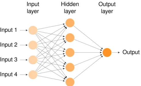
In recent years, benefiting from the rapid development of deep learning technology, the computer vision field has achieved unprecedented success. As one of the most widely used neural networks, Convolutional neural networks (CNNs) are the core learning al-gorithms for visual pattern recognition. They were developed from perceptrons, vector-mapping algorithms inspired by associative learning of the brain, and the idea of “integrate and fire” neurons. Researchers have employed CNNs and their variants (e.g., ResNet) to tackle a variety of challenges such as image classification, object recognition, action recognition, pose estimation, neural style transfer, etc. Previous studies have shown that they outperform humans in some recognition tasks.

Figure 2.1 illustrates a typical architecture of convolutional neural networks. In detail, CNNs are composed of multiple neural units, which can be generally divided into three types, namely, the input layer, the hidden layer and the output layer. The input layer of a convolutional neural network is mainly used to obtain input information, which can process multidimensional data. For example, one-dimensional data is usually time or sampled spectrum, while two-dimensional data may contain multiple channels, such as a three-channel color image, and three-dimensional data may be 3D images such as CR and MRI image. In particular, we focus on 2D/2.5D multimodal images in this thesis.

The output layer of a convolutional neural network usually employs a logical function or softmax function to output the classification labels. The practical application varies according to the type of task. For instance, the output layer can be the central coordinates, size, and classification of objects in object detection. In semantic image segmentation, the output layer directly outputs the classification label of each pixel.

In general, each neural unit in the input layer directly connects to the original data, and provides feature information to the hidden layer. Each neural unit in the hidden layer represents different weights for different neural units in the input layer, so it tends to be sensitive to a certain recognition pattern. The values in the output layer vary according to the activation degree of hidden layers, which is the final recognition result of the model. Compared with the input layer and output layer, the hidden layer is more complex because it is designed for abstract feature extraction. It usually includes the convolutional layer, pooling layer and fully connected layer. In Section 2.2, we introduce the common layers in CNNs.

2.1.3/ ENCODER-DECODER ARCHITECTURE

A convolutional encoder-decoder network is a standard architecture used for tasks requir-ing dense pixel-wise predictions. Such neural network design pattern is frequently used in semantic image segmentation, which is partitioned into two parts, theencoderand the

decoder. Figure 2.2 shows a typical example of the encoder-decoder architecture. In general, an encoder takes the image input and progressively computes higher-level abstract features. The role of the encoder is to encode the low-level image features into a high-dimensional feature vector. The spatial resolution of the feature maps is reduced progressively via the down-sampling operation. Multiple common backbone networks such as VGG, Inception, and ResNet, can be employed for abstract feature extraction in the encoder. The extracted semantic information is then passed into the decoder to com-pute feature maps of progressively increasing resolution via un-pooling or up-sampling. The decoder restores the learned valuable feature representation into a pixel-level seg-mentation mask, which is one of the reasons why the encoder-decoder architecture can be effectively used for image segmentation tasks.

Besides, different variations of the encoder-decoder architecture have been explored to improve the segmentation performance. To name a few, skip connections [150] have been used to recover the fine spatial details during decoding which get lost due to suc-cessive down-sampling operations involved in the encoder. Moreover, larger context in-formation using image-level features [115], recurrent connections [139, 215], and larger convolutional kernels [135] has also significantly improved the accuracy of semantic seg-mentation.

2.2. NEURAL NETWORK LAYERS 15

Figure 2.2: Example of the encoder-decoder architecture.

2.2/

N

EURAL

N

ETWORK

L

AYERS 2.2.1/ CONVOLUTION LAYER

Convolutional layers are the primary building blocks used in convolutional neural net-works. The convolution as a filter enables the neural network to extract effective high-level features. The feature map, also called the activation map, can be generated by repeatedly applying the same filter, which indicates the locations and strength of detected features in the input image. The filter contains the weights that must be learned during the training of the layer. Moreover, the filter size or kernel size will significantly affect the shape of the output feature map. It is worth noting that the interaction of the filter with the border of the image may lead to border effects, especially for the small size input image and very deep network. Usually, we can fix the border effect problem by adding extra pixels to the edge of the image, which is calledpadding. Besides, the amount of movement between the filter applications to the input image is referred to as thestride, and it is almost always symmetrical in height and width dimensions. For example, the stride (2, 2) means moving the filter two pixels right for each horizontal movement of the filter and two pixels down for each vertical movement of the filter when creating the feature map. The stride of the filter on the input image can be seen as the downsampling of the output feature map.

Next, we introduce three essential properties of the convolutional layers: sparse interac-tions, parameter sharing, and equivariant representations.

Sparse interactions Convolutional neural networks have sparse interactions by making the kernel smaller than the input. When processing an image with thousands of pixels, we can detect small valuable features such as the edges of the image by taking only tens to hundreds of pixels. This not only reduces the storage requirements of the model but also improves its overall computation efficiency.

Parameter sharing Parameter sharing is the sharing of weights by all neurons in a par-ticular feature map. Each neuron is connected only to a subset of the input image, which

7 9 3 5 9 4 0 7 0 0 9 0 5 0 9 3 7 5 9 2 9 6 4 3 2 × 2max pooling 9 5 9 9 9 7 2 2

Figure 2.3: Example of max pooling operation.

is also called local connectivity. This property helps to reduce the number of parameters in the whole system and makes the computation more efficient.

Equivariant representations For convolution operation, parameter sharing makes the neural network layers have an equivariant representation. Namely, if the input is slightly shifted, the result of the convolution operation is the same. Note that the convolution is not naturally equivalent to some other transformations such as image scaling or rotation transformation.

2.2.2/ POOLING LAYER

Pooling operation plays a vital role in the structure of convolutional neural networks. First of all, pooling layers improve the spatial invariance to some extent, such as translation invariance, scale invariance, and deformation invariance. Namely, even if the image input is transformed slightly, the pooling layer can still produce similar pooling features, making the learning system more robust. Secondly, pooling operation is equivalent to feature downsampling, which increases the receptive field size. For some visual tasks, a large receptive field helps learn long-range spatial relationships and implicit spatial models. In addition, pooling operation greatly reduces the model parameters, which leads to a lower risk of overfitting. Suppose that the dimension of the image input is c × w × h, where c is the number of channels, and w and h are the width and height, respectively. If the stride of the pooling layer is set to 2, the dimension of the output image will be c × w/2 × h/2. In this case, both the computational cost and memory consumption will be reduced by a factor of 4.

Common pooling methods include average pooling and maximum pooling. Maximum pooling calculates the maximum value of the target patch, which retains more texture information of the image input, whereas average pooling keeps more background infor-mation and tends to transfer the comprehensive inforinfor-mation in the architecture of

convo-2.2. NEURAL NETWORK LAYERS 17 −10 −5 5 10 0.2 0.4 0.6 0.8 1 x y

(a) Sigmoid function.

−6 −4 −2 2 4 6 1 2 3 4 5 x y (b) ReLu function.

Figure 2.4: Examples of popular activation functions.

lutional neural networks. Figure 2.3 shows an example of 2 × 2 maximum pooling.

2.2.3/ RELU LAYER

In neural networks, the activation function performs the nonlinear transformation to the input, making it capable of learning and performing more complex tasks. In order to increase the nonlinearity of neural networks, some nonlinear functions are introduced. Obviously, the accumulation of multiple linear functions is still linear, while linear func-tions have limited expression. The use of nonlinear funcfunc-tions makes the network more expressive and thus better fits the target function. Two common nolinear function used in convolutional neural networks are thesigmoid functionand therectified linear unit(ReLU). As shown in Figure 2.4, we can observe that the ReLU activation function has more advantages than the sigmoid function. ReLU can carry out negative suppression so as to be more sparsely active. More importantly, ReLU activation functions suffer less from the vanishing gradient problem. The derivative of the sigmoid function has good activation only when it is near zero. The gradient in the positive and negative saturation region is close to zero. Also, the derivative of the ReLU function is easy to calculate, which can accelerate the model training to some extent.

2.2.4/ FULLY CONNECTEDLAYER

The fully connected layer is usually used as a classifier to connect the hidden layer and the final output. In the architecture of convolutional neural networks, adding several fully connected layers after the convolution layers can map the generated feature map into a fixed-length feature vector. The final output represents the numerical description of the input image. This structural property is conducive to the realization of image-level

classification and regression tasks.

Although multiple fully connected layers can significantly improve the nonlinear expres-sion ability of learning models, a large number of neurons increase the model complexity. Plenty of model parameters will reduce the efficiency of the learning algorithm and even lead to overfitting. Therefore, the trade-off between accuracy and efficiency has been deeply explored in deep learning technology research. For the segmentation task, how-ever, spatial information should be stored to make a pixel-wise classification. Hence, the fully connected layer is usually substituted by another convolution layer with a large receptive field.

2.3/

O

PTIMIZATION

2.3.1/ BATCH NORMALIZATION

Training deep neural networks with multiple hidden layers is quite challenging. One rea-son is that the model is updated layer-by-layer backward from the output to the input using an error estimate that assumes the weights in the layers prior to the current layer are fixed. This slows down the training by requiring lower learning rates and careful parameter initialization and makes it notoriously hard to train models with saturating non-linearities [79]. Therefore batch normalization, as an effective optimization technique, is proposed to standardize the inputs to a layer for each mini-batch while training very deep neural networks. It stabilizes the learning process and dramatically reduces the number of training epochs required to train deep networks.

Batch normalization can be implemented during training by calculating the mean and standard deviation of each input variable to a layer per mini-batch and using these statis-tics to perform the standardization. Alternatively, a running average of mean and standard deviation can be maintained across mini-batches but may result in unstable training. For example, He et al. [72] used batch normalization after the convolutional layers in their very deep model, referred to as ResNet. The reported results achieved state-of-the-art in the image classification task. In our work of model design, we usually add batch normal-ization transformation before nonlinearity.

2.3.2/ DROPOUT

Deep neural networks are likely to get overfitting while training with few examples. As early as 2012, Hinton et al. [74] has proposed the concept of dropout, which is now widely used in advanced neural networks. Probabilistically dropping out nodes in the network is a simple and effective regularization method [169]. In each iteration, some nodes are

2.4. MODEL TRAINING 19

randomly deleted, and only the remaining nodes are trained. This optimization method reduces the correlation between nodes and the complexity of the model to achieve the effect of regularization.

Generally, dropout only needs to set a hyper-parameter that is the proportion of nodes randomly preserved in each layer. Namely, the parameter matrix of this layer is calculated with the binary matrix generated by the hyper-parameter via the point by point product. Suppose that the hyper-parameter is set to 0.7, then 30% of the nodes will be randomly ignored and produce no outputs from the layer. A good value for dropout in a hidden layer is between 0.5 and 0.8. Input layers use a larger dropout rate, such as of 0.8.

2.4/

M

ODEL

T

RAINING

The process of training neural networks is the most challenging part of using deep learn-ing techniques and is by far the most time consumlearn-ing, both in terms of effort required for configuration and computational complexity required for execution. In the following, we summarize the commonly used techniques in model training, including data preprocess-ing, weight initialization, loss function and gradient descent optimization.

2.4.1/ DATA PREPROCESSING

Generally, training deep learning models requires a lot of data because of the huge num-ber of parameters needed to be tuned by the learning algorithm. Data preprocessing is a prerequisite guarantee for effectively model training, and we need to be careful to prepare the training data to achieve the best prediction results. For example, many deep learning models have normalized input processing, namely whitening operation, which changes the average pixel value of the image to zero and the variance of the image to unit variance. In detail, the mean and variance of the original image are first calculated, then each pixel value of the original image is transformed. This operation enables the convergence of the neural network faster. Common data preprocessing methods also include data quality assessment, feature aggregation, feature sampling, dimensionality reduction, and feature encoding.

Besides, data augmentation [160] is frequently used in model training, which increases the amount of input data by adding slightly modified copies of already existing data or newly created synthetic data from existing data. In the real world scenarios, we may have a small-scale dataset of images taken in a limited set of conditions. In the case of limited data, data augmentation can increase the diversity of training samples, so as to improve the robustness of the model and avoid overfitting. Typical operations include flipping, rotation, shift, resize, random scale, random crop, color jittering, contrast, noise,

fancy PCA, GAN, etc.

2.4.2/ WEIGHT INITIALIZATION

Training a deep learning model means learning good values for all the weights and the bias from labeled examples. In particular, the bias allows to shift the activation function by adding a constant. In order to consistently update the weights, the models require each parameter to have the corresponding initial value. For convolutional neural networks, the nonlinear function is superimposed by multiple layers, and how to select the initial value of parameters becomes a problem worthy of discussion.

In general, the purpose of weight initialization [57, 121] is to prevent the layer activation output from exploding or disappearing in the forward transfer process of deep neural networks. In either case, the loss gradient is either too large or too small to flow backward advantageously. The learning model will then take a longer time to converge. Also, it is notable that initializing all the weights with zeros leads the neurons to learn the same features during training. The model can not get the update of parameters correctly. For example, assume we initialize all the biases to zero and the weights with some constant α. If we forward propagate an input (x1, x2) in the network, the output of hidden layers will

be relu(αx1+ αx2). Namely, the hidden layers will have an identical influence on the cost,

which will result in identical gradients.

In practice, researchers usually employ the Xavier initialization [57] to keep the variance the same across every layer. Another common initialization is He initialization [71], in which the weights are initialized by multiplying by two the variance of the Xavier initializa-tion.

2.4.3/ LOSS FUNCTION

The neural networks are usually trained using the gradient descent optimization algo-rithm. Generally, the optimization problem involves an objective function that indicates the direction of optimization. During the optimization process, the network tries to find a candidate solution to maximize or minimize the objective function. Under constraint conditions, we calculate and minimize the model error via a loss function or cost function, which evaluates the fit of the learning model. This series of constraints is a regularization term that helps to prevent overfitting. The weights are updated using the backpropagation of error algorithm. Therefore we need to choose a suitable loss function when designing and configuring the model.

Suppose that there is a series of training samples {(xi, yi)}i=1,...N in supervised learning.

2.4. MODEL TRAINING 21

in the training samples, it can get the output ˆy as close to the real y as possible. The loss function is a key component to indicate the direction of model optimization, which is used to measure the difference between the output ˆy of the model and the real output y, namely, L= f (yi, ˆyi).

In the following, we introduce several loss functions commonly used for classification and regression in deep learning, including mean squared error loss, mean absolute error loss and cross-entropy loss.

* Mean Squared Error Loss

Mean Squared Error Loss (MSE), also known as Quadratic Loss or L2 Loss, is the

most commonly used loss function in machine learning and deep learning regres-sion tasks. Formally,

JMS E = 1 N N X i=1 (yi− ˆyi)2 (2.6)

Under the assumption that the error between the output of the model and the real value follows a Gaussian distribution, the minimum mean square error loss function and the maximum likelihood estimate are essentially consistent. Therefore, in the scenario where the assumption can be satisfied (such as regression), the mean square error loss is a good choice for the loss function. In scenarios where this assumption is not satisfied (such as classification), other losses have to be consid-ered.

* Mean Absolute Error Loss

Mean Absolute Error Loss (MAE), also known as L1Loss, is another common loss

function. MSE loss generally converges faster than MAE loss, however the latter is more robust to outlier, which can be defined as:

JMAE= 1 N N X i=1 |yi− ˆyi| (2.7) * Cross-Entropy Loss

Previous loss functions introduced above are applicable to regression problems. For classification tasks, especially for semantic image segmentation, the most com-monly used loss function is the cross-entropy loss that increases as the predicted probability diverges from the actual label. For the multi-class cross-entropy loss, we can obtain: JCE = − N X i=1 yci i log( ˆyi ci_{) (2.8)} Here, yci

2.4.4/ GRADIENT DESCENT

A neural network is merely a complicated function, consisting of millions of parameters, that represents a mathematical solution to a problem. By optimizing various parameters of the network, the trained model is finally matched to the learning task under a certain parameter set. The gradient descent method is one of the most commonly used methods to achieve such learning process. In brief, the gradient descent method, also referred to as steepest descent method, is a method to find the minimum of the objective function.

From a mathematical point of view, the gradient indicates the direction of the fastest growth of the function. In other words, the opposite direction of the gradient is the direction of the fastest function decrease. Once we have the direction to move in, we need to decide the size of the step we take. The size of this step is called the learning rate. It is worth noting that if the value of the learning rate is too large, we might overshoot the minima, and keep bouncing along the ridges of the ”valley” without ever reaching the minima. And small learning rate might lead to painfully slow convergence, even get stuck in a minima. The closer the gradient descent method is to the target value, the smaller the step size is and the slower the progress is.

There are three variants of gradient descent, including batch gradient descent, stochas-tic gradient descent, and mini-batch gradient descent. These variants differ in how much data we use to compute the gradient of the objective function. In detail, batch gradient de-scent computes the gradient of the cost function for the entire training dataset. Stochastic gradient descent in contrast performs a weight update for each training example and the corresponding label. As for mini-batch gradient descent, it performs an update for ev-ery mini-batch of n training examples. Taking batch gradient descent as an example, the weight update process can be defined as:

θ := θ − α∇θJ(θ) (2.9)

where J(θ) is the objective function parameterized by the weights θ of the learning model. The parameters is updated in the opposite direction of the gradient of the objective func-tion ∇θJ(θ). The learning rate α determines the size of the steps we take to reach a minimum.

Moreover, several gradient descent optimizers have been proposed, including Momentum SGD, AdaGrad, RMSProp, Adam, etc. For example, Momentum SGD [142] is a method that helps accelerate stochastic gradient descent in the relevant direction and dampens oscillations. It adds a fraction γ of the update vector of the past time step to the current update vector.

2.5. EVALUATION METRICS 23

Then the weights can be updated by θ := θ − vt. The momentum term γ increases for

dimensions whose gradients point in the same directions and reduces updates for dimen-sions whose gradients change directions. As a result, we gain faster convergence and reduced oscillation. Besides, AdaGrad [36] is an alternative algorithm for gradient-based optimization. It adapts the learning rate to the parameters, performs smaller updates for parameters associated with frequently occurring features, and larger updates for in-frequent features. Adaptive Moment Estimation (Adam) [90] is a method that computes adaptive learning rates for each parameter. In addition to storing an exponentially de-caying average of past squared gradients, Adam also keeps an exponentially dede-caying average of past gradients, similar to momentum. Each algorithm has its advantages and disadvantages, we can choose the appropriate optimizer according to the input data and training requirements.

2.5/

E

VALUATION

M

ETRICS

The segmentation performance is generally affected by many factors, such as the pre-processing of data, fusion strategy, the choice of the backbone network, the practice of state-of-the-art deep learning technologies, etc. Therefore how to evaluate and com-pare the performance of segmentation algorithms is a critical issue. The validity and usefulness of a learning system can be measured in many aspects, such as execution time,memory footprint, and accuracy. It is notable that existing large-scale benchmark datasets promote the standardization of comparison metrics, providing a fair comparison of the state-of-the-art methods. In Chapter 3.2.3, we provide a comparative analysis of existing deep multimodal segmentation methods in terms of common metrics.

In general, accuracy is the most common evaluation criteria to measure the perfor-mance of pixel-level prediction [46]. For multimodal image segmentation, the most pop-ular metrics are not different from those used in unimodal approaches, including Pixel Accuracy (PA), Mean Accuracy (MA), Mean Intersection over Union (MIoU), and Fre-quency Weighted Intersection over Union (FWIoU), which are first employed in [117]. In our work, we mainly report a series of segmentation results in Intersection over Union (IoU), also known as the Jaccard Index. The IoU for each category is defined as IoU = T P/(T P + FP + FN), where TP, FP and FN denote true positives, false positives and false negatives, respectively.

For the sake of explanation, we denote ni j as the number of pixels belonging to class i

which are classified into class j, and we consider that there are nclclasses, and ti= Pjni j

is the numbers of pixel in class i. Therefore we can define these accuracy metrics as follows:

• Pixel Accuracy P

inii/ Piti

• Mean Accuracy

(1/ncl)Pinii/ti

• Mean Intersection over Union

(1/ncl)Pinii/(ti+ Pjnji− nii)

• Frequency Weighted Intersection over Union

(P

ktk)−1Pitinii/(ti+ Pjnji− nii)

Besides, researchers usually evaluate the real-time performance of autonomous navi-gation systems by measuring the execution time and memory consumption. Although these indicators are usually closely related to hardware settings, they are also essential for model optimization.

2.6/

S

UMMARY

This chapter reviewed some general concepts in deep learning, including convolution operations and essential neural network layers. This background knowledge laid the foundations for building a compact and efficient convolutional neural network. Especially for the semantic segmentation task, we introduced the encoder-decoder architecture for dense pixel-wise predictions. Besides, several optimization techniques, such as batch normalization and dropout, were stated in detail. Then we presented several standard techniques for neural network training, including data preprocessing, weight initialization, loss function, and gradient descent. Advanced model training strategies were summa-rized in the corresponding section. We highlighted their advantages and disadvantages, which offers the design choice and facilities the model design in our experiments. In the last section, we provided a brief overview of image segmentation evaluation metrics, followed by their mathematical formulations.