RESEARCH OUTPUTS / RÉSULTATS DE RECHERCHE
Author(s) - Auteur(s) :
Publication date - Date de publication :
Permanent link - Permalien :
Rights / License - Licence de droit d’auteur :
Bibliothèque Universitaire Moretus Plantin
Institutional Repository - Research Portal
Dépôt Institutionnel - Portail de la Recherche
researchportal.unamur.be
University of Namur
Exploiting variable precision in GMRES
Gratton, Serge; Simon, Ehouarn; Titley-Peloquin, David; Toint, Philippe
Publication date:
2019
Document Version
Early version, also known as pre-print
Link to publication
Citation for pulished version (HARVARD):
Gratton, S, Simon, E, Titley-Peloquin, D & Toint, P 2019 'Exploiting variable precision in GMRES'.
General rights
Copyright and moral rights for the publications made accessible in the public portal are retained by the authors and/or other copyright owners and it is a condition of accessing publications that users recognise and abide by the legal requirements associated with these rights. • Users may download and print one copy of any publication from the public portal for the purpose of private study or research. • You may not further distribute the material or use it for any profit-making activity or commercial gain
• You may freely distribute the URL identifying the publication in the public portal ? Take down policy
If you believe that this document breaches copyright please contact us providing details, and we will remove access to the work immediately and investigate your claim.
Serge Gratton
∗Ehouarn Simon
†David Titley-Peloquin
‡Philippe Toint
§July 24, 2019
Abstract
We describe how variable precision floating point arithmetic can be used in the iterative solver GMRES. We show how the precision of the in-ner products carried out in the algorithm can be reduced as the iterations proceed, without affecting the convergence rate or final accuracy achieved by the iterates. Our analysis explicitly takes into account the resulting loss of orthogonality in the Arnoldi vectors. We also show how inexact matrix-vector products can be incorporated into this setting.
Keywords— variable precision arithmetic, inexact inner products, inexact
matrix-vector products, Arnoldi algorithm, GMRES algorithm
AMS Subject Codes— 15A06, 65F10, 65F25, 97N20
1
Introduction
As highlighted in a recent SIAM News article [11], there is growing interest in the use of variable precision floating point arithmetic in numerical algorithms. In this paper, we describe how variable precision arithmetic can be exploited in the iterative solver GMRES. We show that the precision of some floating point operations carried out in the algorithm can be reduced as the iterations proceed, without affecting the convergence rate or final accuracy achieved by the iterates.
There is already a literature on the use of inexact matrix-vector products in GM-RES and other Krylov subspace methods; see, e.g., [19, 6, 3, 7, 8] and the references therein. This work is not a simple extension of such results. To illustrate, when per-forming inexact matrix-vector products in GMRES, one obtains an inexact Arnoldi relation
AVk+ Ek= Vk+1Hk, VkTVk= I. (1) ∗INPT-IRIT-ENSEEIHT, Toulouse, France ([email protected]).
†INPT-IRIT-ENSEEIHT, Toulouse, France ([email protected]). The work of
this author was partially supported by the French National program LEFE (Les Enveloppes Fluides et l’Environnement).
‡McGill University, Montreal, Canada ([email protected]). §The University of Namur, Namur, Belgium ([email protected]).
On the other hand, if only inexact inner products are performed, the Arnoldi relation continues to hold exactly, but the orthogonality of the Arnoldi vectors is lost:
AVk= Vk+1Hk, VkTVk= I− Fk. (2)
Thus, to understand the convergence behaviour and maximum attainable accuracy of GMRES implemented in variable precision arithmetic, it is absolutely necessary to understand the resulting loss of orthogonality in the Arnoldi vectors. We adapt techniques used in the rounding-error analysis of the Modified Gram-Schmidt (MGS) algorithm (see [1, 2] or [12] for a more recent survey) and of the MGS-GMRES algo-rithm (see [5, 9, 14]). We also introduce some new analysis techniques. For example, we show that (2) is equivalent to an exact Arnoldi relation in a non-standard inner product, and we analyze the convergence of GMRES with variable precision arithmetic in terms of exact GMRES in this inner product. For more results relating to GMRES in non-standard inner products, see, e.g., [10, 18] and the references therein.
We focus on inexact inner products and matrix-vector products (as opposed to the other saxpy operations involved in the algorithm) because these are the two most time-consuming operations in parallel computations. The rest of the paper is organized as follows. We start with a brief discussion of GMRES in non-standard inner products in Section 2. Next, in Section 3, we analyze GMRES with inexact inner products. We then show how inexact matrix-vector products can be incorporated into this setting in Section 4. Some numerical illustrations are presented in Section 5.
2
GMRES in weighted inner products
Shown below is the Arnoldi algorithm, with⟨y, z⟩ = yTz denoting the standard
Eu-clidean inner product.
Algorithm 1 Arnoldi algorithm Require: A∈ Rn×n, b∈ Rn 1: β =√⟨b, b⟩ 2: v1= b/β 3: for j = 1, 2, . . . do 4: wj= Avj 5: for i = 1, . . . , j do 6: hij=⟨vi, wj⟩ 7: wj= wj− hijvi 8: end for 9: hj+1,j= √ ⟨wj, wj⟩ 10: vj+1= wj/hj+1,j 11: end for
After k steps of the algorithm are performed in exact arithmetic, the output is
Vk+1= [v1, . . . , vk+1]∈ Rn×(k+1) and upper-Hessenberg Hk∈ R(k+1)×ksuch that v1=
b
β, AVk= Vk+1Hk, V T
The columns of Vk form an orthonormal basis for the Krylov subspace Kk(A, b). In
GMRES, we restrict xkto this subspace: xk= Vkyk, where yk∈ Rkis the solution of
min
y ∥b − AVky∥2 = miny ∥Vk+1(βe1− Hky)∥2 = miny ∥βe1− Hky∥2.
It follows that
xk= Vkyk= Vk(HkTHk)−1H T
k(βe1) = VkHk†(βe1), rk= b− Axk= Vk+1(βe1− Hkyk) = Vk+1(I− HkHk†)βe1.
(3) Any given symmetric positive definite matrix W defines a weighted inner product
⟨y, z⟩W = yTW z and associated norm∥z∥W =√⟨z, z⟩W. Suppose we use this inner product instead of the standard Euclidean inner product in the Arnoldi algorithm. We use tildes to denote the resulting computed quantities. After k steps, the result is e
Vk+1= [ev1, . . . ,evk+1] and upper-Hessenberg eHk∈ R(k+1)×ksuch that
ev1= b ∥b∥W = b e β, A eVk= eVk+1 e Hk, VekTW eVk= Ik.
The columns of eVk form a W -orthonormal basis for Kk(A, b). Let exk = eVkeyk, where
eyk∈ Rkis the solution of
min
y ∥b − AeVky∥W = miny ∥eVk+1( eβe1− eHky)∥W = miny ∥eβe1− eHky∥2,
so that
exk= eVkHek†( eβe1), erk= b− Aexk= eVk+1(I− eHkHek†) eβe1.
We denote the above algorithm W -GMRES.
The following lemma shows that if κ2(W ) is small, the Euclidean norm of the
residual vector in W -GMRES converges at essentially the same rate as in standard GMRES. The result is known; see e.g. [18]. We include a proof for completeness.
Lemma 1. Let xk and exk denote the iterates computed by standard GMRES and W -GMRES, respectively, with corresponding residual vectors rkanderk. Then
1≤ ∥erk∥2
∥rk∥2 ≤
√
κ2(W ). (4)
Proof. Both xkandexklie in the same Krylov subspace,Kk(A, b). Because xkis chosen
to minimize the Euclidean norm of the residual inKk(A, b), while exk minimizes the W -norm of the residual inKk(A, b),
∥rk∥2 ≤ ∥erk∥2, ∥erk∥W ≤ ∥rk∥W.
Additionally, because for any vector z
σmin(W )≤ zTW z zTz = ∥z∥2 W ∥z∥2 2 ≤ σmax(W ), we have ∥rk∥2≤ ∥erk∥2 ≤√∥erk∥W σmin(W ) ≤√∥rk∥W σmin(W ) ≤ √ σmax(W ) √ σmin(W ) ∥rk∥2,
3
GMRES with inexact inner products
3.1
Recovering orthogonality
We will show that the standard GMRES algorithm implemented with inexact inner products is equivalent to W -GMRES implemented exactly, for some well-conditioned matrix W . To this end, we need the following theorem.
Theorem 1. Consider a given matrix Q∈ Rn×kof rank k such that
QTQ = Ik− F. (5)
If∥F ∥2 ≤ δ for some δ ∈ (0, 1), then there exists a matrix M such that In+ M is symmetric positive definite and
QT(In+ M )Q = Ik. (6)
In other words, the columns of Q are exactly orthonormal in an inner product defined by In+ M . Furthermore,
κ2(In+ M )≤
1 + δ
1− δ. (7)
Proof. Note from (5) that the singular values of Q satisfy
( σi(Q))2= σi(QTQ) = σi(Ik− F ), i = 1, . . . , k. Therefore, √ 1− ∥F ∥2≤ σi(Q)≤ √ 1 +∥F ∥2, i = 1, . . . , k. (8)
Equation (6) is equivalent to the linear matrix equation
QTM Q = Ik− QTQ.
It is straightforward to verify that one matrix M satisfying this equation is
M = (Q†)T(Ik− QTQ)Q†
= Q(QTQ)−1(Ik− QTQ)(QTQ)−1QT.
Notice that the above matrix M is symmetric. It can also be verified using the singular value decomposition of Q that the eigenvalues and singular values of In+ M are
λi(In+ M ) = σi(In+ M ) =
{(
σi(Q))−2, i = 1, . . . , k,
1, i = k + 1, . . . , n,
which implies that the matrix In+ M is positive definite. From the above and (8),
provided∥F ∥2≤ δ < 1, 1 1 + δ ≤ 1 ( σmax(Q) )2 ≤ σi(In+ M )≤ 1 ( σmin(Q) )2 ≤ 1 1− δ, (9) from which (7) follows.
Note that κ2(In+ M ) remains small even for values of δ close to 1. For example,
suppose∥Ik− QTQ∥
2= δ =1/2, indicating an extremely severe loss of orthogonality.
Then κ2(In+ M )≤ 3, so Q still has exactly orthonormal columns in an inner product
defined by a very well-conditioned matrix.
Remark 1. Paige and his coauthors [2, 13, 17] have developed an alternative
mea-sure of loss of orthogonality. Given Q∈ Rn×kwith normalized columns, the measure is∥S∥2, where S = (I +U )−1U and U is the strictly upper-triangular part of QTQ. Ad-ditionally, orthogonality can be recovered by augmentation: the matrix P =[Q(IS−S)
]
has orthonormal columns. This measure was used in the groundbreaking rounding error analysis of the MGS-GMRES algorithm [14]. In the present paper, under the condition ∥F ∥2≤ δ < 1, we use the measure ∥F ∥2 and recover orthogonality in the (I + M ) in-ner product. For future reference, Paige’s approach is likely to be the most appropriate for analyzing the Lanczos and conjugate gradient algorithms, in which orthogonality is quickly lost and∥F ∥2> 1 long before convergence.
3.2
Bounding the loss of orthogonality
Suppose the inner products in the Arnoldi algorithm are computed inexactly, i.e., line 6 in Algorithm 1 is replaced by
hij= vTiwj+ ηij, (10)
with|ηij| bounded by some tolerance. We use tildes to denote the resulting computed quantities. It is straightforward to show that despite the inexact inner products in (10), the relation AVk= Vk+1Hk continues to hold exactly (under the assumption that all
other operations besides the inner products are performed exactly). On the other hand, the orthogonality of the Arnoldi vectors is lost. We have
[b, AVk] = Vk+1[βe1, Hk], Vk+1Vk+1T = Ik+1+ Fk. (11)
The relation between each ηij and the overall loss of orthogonality Fk is very
diffi-cult to understand. To simplify the analysis we suppose that each vj is normalized
exactly. (This is not an uncommon assumption; see, e.g., [1] and [13].) Under this simplification, we have Fk= ¯Uk+ ¯UkT, Uk¯ = [ 0k×1 Uk 01×1 01×k ] , Uk= v1Tv2 . . . vT1vk+1 . .. ... vTkvk+1 , (12) i.e., Uk∈ Rk×kcontains the strictly upper-triangular part of Fk. Define
Nk= η11 . . . η1k . .. . .. ηkk , Rk= h21 . . . h2k . .. . .. hk+1,k . (13)
Following Bj¨orck’s seminal rounding error analysis of MGS [1], it can be shown that
For completeness, a proof of (14) is provided in the appendix. Note that, assuming GMRES has not terminated by step k, i.e., hj+1,j̸= 0 for j = 1, . . . , k, then Rk must
be invertible. Using (14), the following theorem shows how the convergence of GMRES with inexact inner products relates to that of exact GMRES. The idea is similar to [14, Section 5], in which the quantity∥EkRk−1∥F must be bounded, where Ek is a matrix
containing rounding errors.
Theorem 2. Let x(e)k denote the k-th iterate of standard GMRES, performed exactly, with residual vector r(e)k . Now suppose that the Arnoldi algorithm is run with inexact inner products as in (10), so that (11)–(14) hold, and let xkand rkdenote the resulting GMRES iterate and residual vector. If
∥NkR−1 k ∥2 ≤
δ
2 (15)
for some δ∈ (0, 1), then
1≤ ∥rk∥2 ∥r(e) k ∥2 ≤ √ 1 + δ 1− δ. (16)
Proof. Consider the matrix Fkin (11). From (12) and (14), we have
∥Fk∥2≤ 2∥Uk∥2= 2∥NkRk−1∥2. (17)
Thus, if (15) holds, ∥Fk∥2 ≤ δ < 1 and we can apply Theorem 1 with Q = Vk+1.
There exists a symmetric positive definite matrix W = In+ M such that
[b, AVk] = Vk+1[βe1, Hk], Vk+1W Vk+1T = Ik+1, κ2(W )≤
1 + δ 1− δ.
The Arnoldi algorithm implemented with inexact inner products has computed an
W -orthonormal basis for Kk(A, b). The iterate xk is the same as the iterate that
would have been obtained by running W -GMRES exactly. The result follows from Lemma 1.
3.3
A strategy for bounding the η
ijThe challenge in applying Theorem 2 is bounding the tolerances ηijat step j to ensure
that (15) holds for all subsequent iterations k. Theorem 3 below leads to a practical strategy for bounding the ηij. We will use
tk= βe1− Hkyk
to denote the residual computed in the GMRES subproblem at step k. We will use the known fact that for j = 1, . . . , k,
|eT
jyk| ≤ ∥Hk∥† 2∥tj−1∥2. (18)
This follows from
eTjHk† [ Hj−1 0 0 0 ] | {z } ∈R(k+1)×k [ yj−1 0k−j+1 ] = eTjHk†Hk [ yj−1 0 ] = eTj [ yj−1 0 ] = 0,
and thus |eT jyk| = |e T jHk†β1e1| = eT jHk† ( β1e1− [ Hj−1 0 0 0 ] [ yj−1 0 ]) = eTjHk† [ β1e1− Hj−1yj−1 0 ] ≤ ∥Hk∥† 2∥tj−1∥2.
Additionally, in order to understand how ∥Fk∥2 increases as the residual norm
de-creases, we will need the following rather technical lemma, which is essentially a special case of [15, Theorem 4.1]. We defer its proof to the appendix.
Lemma 2. Let ykand tk be the least squares solution and residual vector of
min
y ∥βe1− Hky∥2. Given ϵ > 0, let Dk be any nonsingular matrix such that
∥Dk∥2≤ σmin(Hk)ϵ∥b∥2 √ 2∥tk∥2 . (19) Then ∥tk∥2 ( ϵ2∥b∥2 2+ 2∥Dkyk∥22 )1/2 ≤ σmin ([ ϵ−1e1, HkD−1k ]) ≤ ∥tk∥2 ϵ∥b∥2 . (20)
Theorem 3. In the notation of Theorem 2 and Lemma 2, if for all steps j = 1, . . . , k of
GMRES all inner products are performed inexactly as in (10) with tolerances bounded by |ηij| ≤ ηj≡ϕjϵσmin√ (Hk) 2 ∥b∥2 ∥tj−1∥2 (21)
for any ϵ∈ (0, 1) and any positive numbers ϕj such that∑kj=1ϕ2j≤ 1, then at step k either (16) holds with δ =1/2, or
∥tk∥2 ∥b∥2 ≤ 6kϵ,
(22)
implying that GMRES has converged to a relative residual of 6kϵ.
Proof. If (21) holds, then in (13)
|Nk| ≤ η1 η2 . . . ηk η2 . . . ηk . .. . .. ηk = EkDk,
where Ek is an upper-triangular matrix containing only ones in its upper-triangular
part, so that∥Ek∥2≤ k, and Dk= diag(η1, . . . , ηk). Then in (15), ∥NkR−1
k ∥2≤ ∥NkDk−1∥2∥DkRk−1∥2
≤ ∥Ek∥2∥DkR−1k ∥2≤ k∥(RkD−1k )−1∥2.
Let hT
k denote the first row of Hk, so that Hk=
[
hTk Rk
]
. For any ϵ > 0 we have
σmin(RkDk−1) = min ∥u∥2=∥v∥2=1 uTRkD−1k v = min ∥u∥2=∥v∥2=1 [0, uT] [ ϵ−1 hTkD−1k 0 RkD−1k ] [ 0 v ] ≥ min ∥u∥2=∥v∥2=1 uT [ ϵ−1 hTkD−1k 0 RkDk−1 ] v = σmin ([ ϵ−1e1, HkD−1k ]) . Therefore, ∥(RkD−1 k )−1∥2= 1 σmin(RkD−1k ) ≤ 1 σmin ([ ϵ−1e1, HkD−1k ]) .
Notice that if the ηjare chosen as in (21), Dk automatically satisfies (19). Using the
lower bound in Lemma 2, and then (18) and (21), we obtain
∥(RkD−1 k )−1∥2≤ ( ϵ2∥b∥2 2+ 2∥Dkyk∥22 )1/2 ∥tk∥2 = ( ϵ2∥b∥2 2+ 2 ∑k j=1η 2 j(eTjyk)2 )1/2 ∥tk∥2 ≤ ( ϵ2∥b∥2 2+ ∑k j=1ϕ 2 jϵ2∥b∥22 )1/2 ∥tk∥2 = √ 2ϵ∥b∥2 ∥tk∥2 . Therefore, in (23), ∥NkR−1 k ∥2≤ √ 2kϵ∥b∥2 ∥tk∥2 ≤ 6kϵ∥b∥2 ∥tk∥2 δ 2 with δ =1/2. If (22) does not hold, then∥NkR−1
k ∥2 ≤ δ/2, which from Theorem 2
implies (16). Therefore, if the|ηij| are bounded by tolerances ηj chosen as in (21), either (16) holds with δ =1/2, or (22) holds.
Theorem 3 can be interpreted as follows. If at all steps j = 1, 2, . . . of GMRES the inner products are computed inaccurately with tolerances ηjin (21), then convergence
at the same rate as exact GMRES is achieved until a relative residual of essentially kϵ is reached. Notice that ηjis inversely proportional to the residual norm. This allows
the inner products to be computed more and more inaccurately as as the iterations proceed.
If no more than Kmax iterations are to be performed, we can let ϕj = K−
1/2
max
(although more elaborate choices for ϕj could be considered; see for example [8]).
Then the factorϕj/√2in (21) can be absorbed along with the k in (22).
One important difficulty with (21) is that σmin(Hk) is required to pick ηj at the
start of step j, but Hk is not available until the final step k. A similar problem
occurs in GMRES with inexact matrix-vector products; see [19, 6] and the comments in Section 4. In our experience, is often possible to replace σmin(Hk) in (21) by 1,
without significantly affecting the convergence of GMRES. This leads to following: Aggressive threshhold : ηj= ϵ ∥b∥2
∥tj−1∥2
In exact arithmetic, σmin(Hk) is bounded below by σmin(A). If the smallest singular
value of A is known, one can estimate σmin(Hk) ≈ σmin(A) in (21), leading to the
following:
Conservative threshhold : ηj= ϵ σmin(A) ∥b∥ 2 ∥tj−1∥2
, j = 1, 2, . . . . (25) This prevents potential early stagnation of the residual norm, but is often unnecessarily stringent. (It goes without saying that if the conservative threshold is less than u∥A∥2,
where u is the machine precision, then the criterion is vacuous: according to this criterion no inexact inner products can be carried out at iteration j.) Numerical examples are given in Section 5.
4
Incorporating inexact matrix-vector products
As mentioned in the introduction, there is already a literature on the use of inexact matrix-vector products in GMRES. These results are obtained by assuming that the Arnoldi vectors are orthonormal and analyzing the inexact Arnoldi relation
AVk+ Ek= Vk+1Hk, VkTVk= I.
In practice, however, the computed Arnoldi vectors are very far from being orthonor-mal, even when all computations are performed in double precision arithmetic; see for example [5, 9, 14].
The purpose of this section is to show that the framework used in [19] and [6] to analyze inexact matrix-vector products in GMRES is still valid when the orthogonality of the Arnoldi vectors is lost, i.e., under the inexact Arnoldi relation
AVk+ Ek= Vk+1Hk, VkTVk= I− Fk. (26)
This settles a question left open in [19, Section 6].
Throughout we assume that∥Fk∥2≤ δ < 1. Then from Theorem 1 there exists a
symmetric positive definite matrix W = In+M∈ Rn×nsuch that Vk+1W Vk+1T = Ik+1,
and with singular values bounded as in (9).
4.1
Bounding the residual gap
As in previous sections, we use xk = Vkyk to denote the computed GMRES iterate,
with rk= b− Axkfor the actual residual vector and tk= β1e1− Hkykfor the residual
vector updated in the GMRES iterations. From
∥rk∥2≤ ∥rk− Vk+1tk∥2+∥Vk+1tk∥2, if max{ ∥rk− Vk+1tk∥2,∥Vk+1tk∥2} ≤ ϵ 2∥b∥2 (27) then ∥rk∥2≤ ϵ∥b∥2. (28)
From the fact that the columns of W1/2Vk+1are orthonormal as well as (9), we obtain
∥Vk+1tk∥2≤ ∥W− 1/2∥ 2∥W 1/2Vk+1tk∥ 2=∥W ∥− 1/2 2 ∥tk∥2≤ √ 1 + δ∥tk∥2.
In GMRES,∥tk∥2→ 0 with increasing k, which implies that ∥Vk+1tk∥2 → 0 as well.
Therefore, we focus on bounding the residual gap∥rk−Vk+1tk∥2in order to satisfy (27)
and (28).
Suppose the matrix-vector products in the Arnoldi algorithm are computed inex-actly, i.e., line 4 in Algorithm 1 is replaced by
wj= (A +Ej)vj, (29)
where∥Ej∥2≤ ϵjfor some given tolerance ϵj. Then in (26), Ek=[E1v1,E2v2, . . . ,Ekvk
]
. (30)
The following theorem bounds the residual gap at step k in terms of the tolerances δ and ϵj, for j = 1, . . . , k.
Theorem 4. Suppose that the inexact Arnoldi relation (26) holds, where Ekis given in (30) with ∥Ej∥2 ≤ ϵj for j = 1, . . . , k, and ∥Fk∥2 ≤ δ < 1. Then the resulting residual gap satisfies
∥rk− Vk+1tk∥2≤ ∥Hk∥† 2 k
∑
j=1
ϵj∥tj−1∥2. (31) Proof. From (26) and (30),
∥rk− Vk+1tk∥2=∥b − AVkyk− Vk+1tk∥2 =∥b − Vk+1Hkyk+ Ekyk− Vk+1tk∥2 =∥Vk+1(β1e1− Hkyk) + Ekyk− Vk+1tk∥2 =∥Ekyk∥2 = k ∑ j=1 EjvjeT jyk 2 ≤ k ∑ j=1 ϵj|eT jyk|.
The result then follows from (18).
4.2
A strategy for picking the ϵ
jTheorem 4 suggests the following strategy for picking the tolerances ϵj that bound
the level of inexactness ∥Ej∥2 in the matrix-vector products in (29). Similarly to
Theorem 3, let ϕj be any positive numbers such that
∑k
j=1ϕj = 1. If for all steps j = 1, . . . , k, ϵj≤ϕjϵσmin(Hk) 2 ∥b∥2 ∥tj−1∥2 , (32)
then from (31) the residual gap in (27) satisfies
∥rk− Vk+1tk∥2≤ ϵ
2∥b∥2.
Interestingly, this result is independent of δ. Similarly to (21), the criterion for picking
ϵj at step j involves Hk that is only available at the final step k. A large number
of numerical experiments [6, 3] indicate that σmin(Hk) can often be replaced by 1.
Absorbing the factorϕj/2 into ϵ in (32) and replacing σmin(Hk) by 1 or by σmin(A)
leads, respectively, to the same aggressive and conservative thresholds for ϵj as we
obtained for ηj in (24) and in (25). This suggests that matrix-vector products and
inner products in GMRES can be computed with the same level of inexactness. We illustrate this with numerical examples in the next section.
5
Numerical examples
We illustrate our results with a few numerical examples. We run GMRES with different matrices A and right-hand sides b, and compute the inner products and matrix-vector products inexactly as in (10) and (29). We pick ηij randomly, uniformly distributed
between −ηj and ηj, and pick Ej to be a matrix of independent standard normal
random variables, scaled to have norm ϵj. Thus we have |ηij| ≤ ηj, ∥Ej∥2≤ ϵj,
for chosen tolerances ηj and ϵj. Throughout we use the same level of inexactness for
inner products and matrix-vector products, i.e., ηj= ϵj.
In our first example, A is the 100×100 Grcar matrix of order 5. This is a highly non-normal Toeplitz matrix. The right hand side is b = A[sin(1), . . . , sin(100)]T. Results are shown in Figure 1. The solid green curve is the relative residual∥b − Axk∥2/∥b∥2.
For reference, the dashed blue curve is the relative residual if GMRES is run in double precision. The full magenta curve corresponds to the loss of orthogonality ∥Fk∥2
in (11). The black dotted curve is the chosen tolerance ηj.
In Example 1(a), ηj= ϵj= 10−8∥A∥2, for 20≤ j ≤ 30, 10−4∥A∥2, for 40≤ j ≤ 50, 2−52∥A∥2, otherwise.
The large increase in the inexactness of the inner products at iterations 20 and 40 immediately leads to a large increase in∥Fk∥2. This clearly illustrates the connection
between the inexactness of the inner products and the loss of orthogonality in the Arnoldi vectors. As proven in Theorem 2, until∥Fk∥2 ≈ 1, the residual norm is the
same as it would have been had all computations been performed in double precision. Due to its large increases at iterations 20 and 40,∥Fk∥2approaches 1, and the residual
norm starts to stagnate, long before a backward stable solution is obtained.
In Example 1(b), the tolerances are chosen according to the aggressive crite-rion (24) with ϵ = 2−52∥A∥2. With this judicious choice, ∥Fk∥2 does not reach 1,
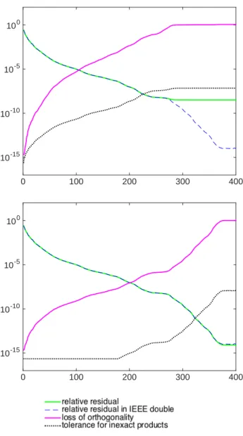
and the residual norm does not stagnate, until a backward stable solution is obtained. In our second example, A is the matrix 494 bus from the SuiteSparse matrix col-lection [4]. This is a 494× 494 matrix with condition number κ2(A)≈ 106. The right
hand side is once again b = A[sin(1), . . . , sin(100)]T.
Results are shown in Figure 2. In Example 2(a), tolerances are chosen according to the aggressive threshhold (24) with ϵ = 2−52∥A∥2. In this more ill-conditioned
problem, the residual norm starts to stagnate before a backward stable solution is obtained. In Example 2(b), the tolerances are chosen according to the conservative threshhold (25) with ϵ = 2−52∥A∥2, and there is no more such stagnation. Because
of these lower tolerances, the inner products and matrix-vector products have to be performed in double precision until about iteration 200. This example illustrates the tradeoff between the level of inexactness and the maximum attainable accuracy. If one requires a backward stable solution, the more ill-conditioned the matrix A is, the less opportunity there is for performing floating-point operations inexactly in GMRES.
Example 1(a) 0 20 40 60 80 100 10-15 10-10 10-5 100 Example 1(b) 0 20 40 60 80 100 10-15 10-10 10-5 100
Figure 1: GMRES in variable precision: Grcar matrix.
6
Conclusion
We have shown how inner products can be performed inexactly in MGS-GMRES without affecting the convergence or final achievable accuracy of the algorithm. We have also shown that a known framework for inexact matrix-vector products is still valid despite the loss of orthogonality in the Arnoldi vectors. It would be interesting to investigate the impact of scaling or preconditioning on these results. Additionally,
Example 2(a) 0 100 200 300 400 10-15 10-10 10-5 100 Example 2(b) 0 100 200 300 400 10-15 10-10 10-5 100
Figure 2: GMRES in variable precision: 494 bus matrix
in future work, we plan to address the question of how much computational savings can be achieved by this approach on massively parallel computer architectures.
Appendix
A
Proof of (14)
In line 7 of Algorithm 1, in the ℓth pass of the inner loop at step j, we have
w(ℓ)j = w(ℓj−1)− hℓjvℓ (A1) for ℓ = 1, . . . , j and with w(0)j = Avj. Writing this equation for ℓ = i + 1 to j, we have
w(i+1)j = w(i)j − hi+1,jvi+1,
w(i+2)j = w(i+1)j − hi+2,jvi+2,
.. .
w(j)j = w(jj−1)− hj,jvj.
Summing the above and cancelling identical terms that appear on the left and right hand sides gives
w(j)j = w (i) j − j ∑ ℓ=i+1 hℓjvℓ.
Because wj(j)= vj+1hj+1,j, this reduces to
wj(i)= j+1
∑
ℓ=i+1
hℓjvℓ. (A2)
Because the inner products hijare computed inexactly as in (10), from (A1) we have wj(i)= w (i−1) j − hijvi = wj(i−1)− (v T iw (i−1) j + ηij)vi = (I− vivTi)w (i−1) j − ηijvi. Therefore, viTw (i) j =−ηij.
Multiplying (A2) on the left by−vTi gives
ηij=−
j+1
∑
ℓ=i+1
hℓj(viTvℓ), (A3)
which is the entry in position (i, j) of the matrix equation η11 . . . η1k . .. . .. ηkk = − vT 1v2 . . . vT1vk+1 . .. . .. vTkvk+1 h21 . . . h2k . .. . .. hk+1,k , i.e., (14).
B
Proof of Lemma 2
For any γ > 0, the smallest singular value of the matrix[βγe1, HkD−1k
]
is the scaled total least squares (STLS) distance [16] for the estimation problem HkD−1k z ≈ βe1.
As shown in [15], it can be bounded by the least squares distance min
z ∥βe1− HkD −1
k z∥2=∥βe1− HkD−1k zk∥2=∥βe1− Hkyk∥2=∥tk∥2,
where zk= Dkyk. From [15, Theorem 4.1], we have ∥tk∥2 ( γ−2+∥Dkyk∥2 2/(1− τk2) )1/2 ≤ σmin ([ βγe1, HkDk−1 ]) ≤ γ∥tk∥2, (B1) provided τk< 1, where τk≡σmin ([ βγe1, HkD−1k ]) σmin ( HkD−1k ) .
We now show that if γ = (ϵ∥b∥2)−1 and Dk satisfies (19), then τk ≤1/√2. From the
upper bound in (B1) we immediately have
σmin ([ βγe1, HkD−1k ]) ≤ γ∥tk∥2= ∥tk∥ 2 ϵ∥b∥2 . Also, σmin ( HkD−1k ) = min z̸=0 ∥HkD−1 k z∥2 ∥z∥2 = min z̸=0 ∥Hkz∥2 ∥Dkz∥2 ≥ minz̸=0 ∥Hkz∥2 ∥Dk∥2∥z∥2 = σmin(Hk) ∥Dk∥2 . Therefore, if (19) holds, τk≤ ∥tk∥2 ϵ∥b∥2 ∥Dk∥2 σmin(Hk) ≤ √1 2. Substituting γ = (ϵ∥b∥2)−1 and τk≤1/√2into (B1) gives (20).
References
[1] A. Bj¨orck, Solving linear least squares problems by Gram-Schmidt
orthogonal-ization, BIT Numerical Mathematics, 7 (1967), pp. 1–21.
[2] A. Bj¨orck and C. Paige, Loss and recapture of orthogonality in the Modified
Gram-Schmidt algorithm, SIAM Journal on Matrix Analysis and Applications, 13
(1992), pp. 176–190.
[3] A. Bouras and V. Frayss´e, Inexact matrix-vector products in Krylov
meth-ods for solving linear systems: A relaxation strategy, SIAM Journal on Matrix
Analysis and Applications, 26 (2006), pp. 660–678.
[4] T. A. Davis and Y. Hu, The University of Florida sparse matrix collection, ACM Transactions on Mathematical Software, 38 (2011), pp. 1–25.
[5] J. Drkoˇsov´a, A. Greenbaum, M. Rozloˇzn´ık, and Z. Strakoˇs, Numerical
stability of GMRES, BIT Numerical Mathematics, 35 (1995), pp. 309–330.
[6] J. V. D. Eshof and G. Sleijpen, Inexact Krylov subspace methods for linear
systems, SIAM Journal on Matrix Analysis and Applications, 26 (2004), pp. 125–
[7] L. Giraud, S. Gratton, and J. Langou, Convergence in backward error of
relaxed GMRES, SIAM Journal on Scientific Computing, 29 (2007), pp. 710–728.
[8] S. Gratton, E. Simon, and P. Toint, Minimizing convex quadratic with
vari-able precision Krylov methods, arXiv, abs/1807.07476 (2018).
[9] A. Greenbaum, M. Rozloˇzn´ık, and Z. Strakoˇs, Numerical behaviour of the
Modified Gram-Schmidt GMRES implementation, BIT Numerical Mathematics,
37 (1997), pp. 706–719.
[10] S. G¨uttel and J. Pestana, Some observations on weighted GMRES, Numerical Algorithms, 67 (2014), pp. 733–752.
[11] N. J. Higham, A multiprecision world, SIAM News, 50 (2017).
[12] S. J. Leon, A. Bj¨orck, and W. Gander, Gram-Schmidt orthogonalization:
100 years and more, Numerical Linear Algebra with Applications, 20 (2013),
pp. 492–532.
[13] C. Paige, A useful form of unitary matrix obtained from any sequence of unit 2-norm n-vectors, SIAM Journal on Matrix Analysis and Applications, 31 (2009), pp. 565–583.
[14] C. Paige, M. Rozloˇzn´ık, and Z. Strakoˇs, Modified Gram-Schmidt (MGS),
least squares, and backward stability of MGS-GMRES, SIAM Journal on Matrix
Analysis and Applications, 28 (2006), pp. 264–284.
[15] C. Paige and Z. Strakoˇs, Bounds for the least squares distance using scaled
total least squares, Numerische Mathematik, 91 (2002), pp. 93–115.
[16] C. Paige and Z. Strakoˇs, Scaled total least squares fundamentals, Numerische Mathematik, 91 (2002), pp. 117–146.
[17] C. Paige and W. W¨ulling, Properties of a unitary matrix obtained from a
se-quence of normalized vectors, SIAM Journal on Matrix Analysis and Applications,
35 (2014), pp. 526–545.
[18] J. Pestana and A. J. Wathen, On the choice of preconditioner for minimum
residual methods for non-Hermitian matrices, Journal of Computational and
Ap-plied Mathematics, 249 (2013), pp. 57 – 68.
[19] V. Simoncini and D. Szyld, Theory of inexact Krylov subspace methods and
applications to scientific computing, SIAM Journal on Scientific Computing, 25