HAL Id: tel-01572434
https://hal.archives-ouvertes.fr/tel-01572434v2
Submitted on 24 Aug 2017
HAL is a multi-disciplinary open access
archive for the deposit and dissemination of
sci-entific research documents, whether they are
pub-lished or not. The documents may come from
teaching and research institutions in France or
abroad, or from public or private research centers.
L’archive ouverte pluridisciplinaire HAL, est
destinée au dépôt et à la diffusion de documents
scientifiques de niveau recherche, publiés ou non,
émanant des établissements d’enseignement et de
recherche français ou étrangers, des laboratoires
publics ou privés.
Distributed under a Creative Commons Attribution - NonCommercial| 4.0 International
License
approaches for human cell population dynamics
Samuel Bernard
To cite this version:
Samuel Bernard. Structured differential equations and multiscale approaches for human cell
pop-ulation dynamics. Dynamical Systems [math.DS]. Université Claude Bernard Lyon 1, 2017.
�tel-01572434v2�
Institut Camille Jordan
UMR 5208 du CNRS
Structured differential equations and multiscale
approaches for human cell population dynamics
Samuel Bernard
Université Claude Bernard Lyon 1
École doctorale InfoMath, ED 512
Spécialité : Mathématiques
N. d’ordre 034–2017
Structured differential equations and multiscale
approaches for human cell population dynamics
Habilitation à diriger des recherches
Soutenue publiquement le 12 juin 2017 par
Samuel Bernard
devant le Jury composé de:
Mme. Angélique Stéphanou
CR CNRS, Grenoble
ExaminatriceM. Franck Delaunay
PU, Nice
ExaminateurMme Fahima Nekka
PR, Montreal
RapporteurM. Laurent Pujo-Menjouet
MCF, HDR, Lyon 1
ExaminateurM. David Rand
PR, Warwick
RapporteurContents
1
Remerciements
1
2
Curriculum Vitae
5
3
Introduction
15
4 Delay equations
19
4.1
Differential equations with distributed delays
. . . .
20
4.2
G
⟨n⟩[dM]
. . . .
22
4.3
Stability results
. . . .
23
4.4 Positive feedback loops and robustness of oscillations
. . . .
25
5
Circadian clocks
27
5.1
The circadian clock
. . . .
28
5.2
Damped versus sustained oscillators
. . . .
28
5.3
Synchronization of biological oscillators
. . . .
30
5.4
Synchronization of circadian oscillators
. . . .
32
6 Cell proliferation
35
6.1
Birth-and-death models and 14C dating
. . . .
36
6.2
Renewal equations
. . . .
37
6.3
14C model and data
. . . .
39
6.4 Nonlinear fitting strategies
. . . .
39
6.5
Cardiomyocyte renewal in humans
. . . .
40
6.6 Tumor-immune interaction
. . . .
41
7
Integrative approaches
43
7.1
Multiscale modeling in biology
. . . .
44
7.2
The cell division cycle and the circadian clock
. . . .
44
7.3
Circadian clock and liver renewal
. . . .
45
7.4
Modulation of cell population growth under circadian clock control
. . . .
45
7.5
Simuscale
. . . .
46
8 Outlook
49
9 Selected papers
53
9.1
Bernard S, Crauste F (2015) Optimal linear stability condition for scalar differential
equations with distributed delay. Discrete Contin Dynam Systems Ser B 20:1855–
1876
. . . .
55
9.2
Bergmann O, Bhardwaj R, Bernard S, Zdunek S, Barnabé-Heider F, Walsh S,
Zupi-cich J, Alkass K, Buchholz B, Druid H, Jovinge S, Frisén J (2009) Evidence for
car-diomyocyte renewal in humans. Science 324:98–102
. . . .
79
9.3
Bernard S, Gonze D, Čajavec B, Herzel H, Kramer A (2007)
Synchronization-induced rhythmicity of circadian oscillators in the
suprachias-matic nucleus. PLOS Comput Biol 3:e68
. . . .
85
9.4 Besse A, Clapp G, Bernard S, Nicolini F, Levy D, Lepoutre T (2017) Stability analysis
of a model of interaction between the immune system and cancer cells in chronic
myelogenous leukemia. Bull Math Biol in press
. . . .
99
9.5
Chauhan A, Lorenzen S, Herzel H, Bernard S (2011) Regulation of mammalian cell
cycle progression in the regenerating liver. J Theor Biol 283:103–112
. . . .
129
9.6 El Cheikh R, Bernard S, El Khatib N (2014) Modeling circadian clock-cell cycle
in-teraction effects on cell population growth rates. J Theor Biol 363:318–331
. . . . .
141
Chapter 1
Remerciements
There are so many people I would like to thank for making this thesis possible. I am very grateful to
all of you. My first thanks go to the HDR thesis defence committee. To my reviewers, David Rand,
Benoît Perthame and Fahima Nekka, thank you for taking the time to read the thesis carefully and
review it in depth. I would like to thank the examiners, Franck Delaunay, Angélique Stéphanou
and Laurent Pujo-Menjouet for accepting to be part of the defence committee. Having your names
on the thesis cover means a great deal to me.
L’Institut Camille Jordan et le CNRS m’ont soutenu depuis mon arrivée à Lyon en 2007, je les
en remercie. Je remercie aussi la direction de l’ICJ, Frank Wagner et Elisabeth Mironescu par le
passé et maintenant Sylvie Benzoni, ainsi que Simon Masnou, chef de l’équipe MMCS à l’ICJ, pour
leur soutien aux biomathématiques; le support informatique à l’ICJ, Laurent Azema et Thierry
Dumont; et Régis Goiffon pour son enthousiasme à partager les maths à l’Université Ouverte. Je
voudrais remercier le centre Inria Grenoble et sa direction pour l’accueil dans l’équipe Dracula et
son soutien pour le développement de Simuscale, et David Parsons qui s’est investi
personnelle-ment dans ce projet. Un grand merci à l’IXXI pour son soutien financier et à son ex-directeur
Guillaume Beslon, pour avoir promu l’interdisciplinarité en Rhône-Alpes et aidé à créer une
at-mosphère propice à l’épanouissement des biomathématiques. Un grand merci à Mostafa Adimy,
directeur de l’équipe Inria Dracula, qui ne compte pas son temps pour que le nôtre puisse être
consacré à la science.
I have a special thought for my collaborators past and present: Kirsty Spalding, Jonas Frisén, the
14C data is the best application of renewal equations one could think of; Peter Arner, for the
pre-cious data in the freezer; Mikael Rydén, Olaf Bergmann, Hagen Huttner, Aurélie Ernst, such
fruit-ful collaborations; Henrik Druid, Brita Zilg, Kanar Alkass, I can’t watch CSI with the same eye now;
Jeff Mold, Pedro Réu, for the one last question; et Fanie Barnabé-Heider, pour l’accent du Québec à
Stockholm. Didier Gonze, Hanspeter Herzel, Achim Kramer, Francis Lévi, Pål Westermark,
mod-elling the circadian clock raises so much interesting questions; Vitaly Volpert, Nader El Khatib et
Angélique vous avez motivé mon intérêt pour la modélisation multiéchelles/hybride.
La vie de labo ne serait pas la même sans les membres de l’équipe Dracula. Fabien Crauste, Thomas
Lepoutre, Laurent, Céline Vial, Olivier Gandrillon, Léon Tine, vous êtes bien plus que des
col-lègues. Fabien, merci d’y avoir cru quand j’ai eu des doutes. Merci aussi pour ton écoute, tes
conseils et ton aide dans les bons moments comme dans les très mauvais, je n’oublierai pas les
virées à Ikea, par exemple. Laurent, je n’oublierai pas le canot sur le lac Pilon, les papiers écrits
sur la plage à Vancouver, et ton accueil à mon arrivée en France. Il y a aussi toutes celles et ceux
que je croise à la salle café. C’est rassurant de voir qu’on peut toujours y trouver quelqu’un en train
de se faire couler un espresso ou une infusion.
À mes doctorants et les étudiants avec qui j’ai travaillé, ici et ailleurs: Stephan Fischer, Charles
Rocabert, Catherine Foley, Paulina Kurbatova, Pauline Mazzocco, ainsi que tous les stagiaires,
c’est toujours un plaisir de travailler avec vous. Embla Steiner, Sofia Zdunek, thank you for the
stimulating discussions. Apollos Besse, Raouf El Cheikh, Anuradha Chauhan, certains de ces
chapitres n’auraient pas été possibles sans votre travail et votre persévérance. Merci de m’avoir
fait confiance.
To my thesis directors and postdoc supervisors Michael Mackey, Jacques Bélair, Hanspeter, and
Daphne Manoussaki, with whom it all got started. I learned a lot with you, thank you.
Un grand merci à toute l’équipe administrative de l’ICJ, et en particulier à Maria Konieczny, qui
a été de toutes mes aventures administratives avec une bonne humeur indéfectible. Merci
in-finiement à Caroline Lothe pour sa grande patience à mon égard, je sais que je peux m’améliorer.
Merci à Hédi Soula et Hubert Charles pour les opportunités d’enseignement en 3BIM INSA, et à
Anne-Laure Fougères pour avoir pris en charge la direction du Master Maths en Action à l’UCBL.
À ma famille, Roseline, Sophie, Luc, Paul, Mélissa, François, Roxane, Marjolaine et Pierre, qui sont
3
toujours là même de loin. A Dora, Ella et Alex pour leur source inépuisable de joie et d’énergie,
et pour les “tangled monster plots”. Et enfin à Carole, sans qui cette thèse ne serait qu’un projet
flou.
Chapter 2
Curriculum Vitae
Expérience professionnelle
CNRS, France Depuis octobre 2011 Membre de l’Equipe-Projet Dracula, Inria Grenoble Depuis octobre 2007 Chargé de Recherche 1re classe CNRS UMR5208 Institut Camille Jordan, Université de Lyon Marie Curie Research Training Network, Grèce 2006 – 2007 Chercheur Expérimenté (post-doctoral) avec Daphne Manoussaki Marie Curie Research Training Network on Mathematical Methods and Computer Simulation of Tumour Growth and Therapy Institute of Applied and Computational Mathematics Foundation for Research and Technology— Hellas, P.O. Box 1527, 71110 Héraklion, Crète, GrèceInstitute for Theoretical Biology, Germany 2004 – 2006, 2007 Assistant de Recherche (post-doctoral) dans le groupe de Hanspeter Herzel Institute for Theoretical Biology, Université Humboldt, Invalindenstr. 43, 10115 Berlin, Allemagne
Formation académique
Université de Montréal, Canada 2000 – 2003 Ph.D. en Mathématiques Appliquées avec Jacques Bélair (Université de Montréal) et Michael C. Mackey (Université McGill) Équations différentielles à retard et leur application en hématopoïèse, avec étude du cas de la neutropénie cyclique (2003).Domaines d’expertise
Mathématiques Mathématiques appliquées, dynamique non-linéaire, equations différentielles à retard, processus stochastiques, analyse numérique, modélisation de systèmes physiologiques, pharmacodynamique/pharmacocinétique, modélisation multiéchelles Institut Camille Jordan (CNRS UMR5208) Bât. Jean Braconnier, 43 blvd du 11 novembre 1918, F-69622 Villeurbanne-Cedex, France Courriel: [email protected] Web: math.univ-lyon1.fr/~bernard/ Twitter: @samu6ernard Langues parlées: français et anglais courants, allemand intermédiaireBiology théorique Horloge circadienne, désordres hématopoïétiques, cycle cellulaire et croissance tumorale, regulation transcriptionnelle, analyse de données 14C pour le renouvellement de tissus à faible potential régénératifs Programmation Matlab, R, C, C++
Prix & subventions
2013 - aujourd’hui Foreign Adjunct Professor, Institut Karolinska, Stockholm, Suède 2014 - aujourd’hui Coordonnateur pour le projet Inria de développement logiciel software development project (Inria ADT) Simuscale: une plateforme de simulation multiéchelles pour la dynamique de populations cellulaires. https://gforge.inria.fr/projects/simuscale/ 2013-2015 Coordonnateur Partenariat Hubert Curien, Projet Cèdre, Campus France, 30097ZA (18,000 €, 2 years) 2004 Prix de la meilleure thèse en sciences pures et appliquées de l’Université de Montréal remis par la Faculté des Études SupérieuresEnseignement
Dynamique des populations cellulaires (Master 2) Université Lyon 1, 15h par an. http://math.univ-lyon1.fr/homes-www/bernard/popdyn.html Algèbre linéaire et analyse matricielle (3e année de licence) INSA Lyon, 30h par an. http://math.univ-lyon1.fr/homes-www/bernard/numalg.html EDO pour les neurosciences (3e année de licence) INSA Lyon, 10h par an. http://math.univ-lyon1.fr/~bernard/edoneuro.htmlDirection de thèse
2014-2017 Directeur, Apollos Besse, Université Lyon 1 Modélisation mathématique de la leucémie myéloïde chronique et de ses traitements 2011-2015 Co-directeur, Raouf El Cheik, Université Lyon 1application à la chronothérapie 2011-2015 Superviseur scientifique, Sofia Zdunek, Insitut Karolinska, Stockholm Analyse du renouvellement de cellules cardiaque chez l’humain par datation radiocarbone et modélisation mathématique 2010-2013 Co-directeur, Stephan Fischer, INSA Lyon Modélisation de l'évolution de la taille des génomes et de leur densité en gènes par mutations locales et grands réarrangements chromosomiques 2006-2010 Superviseur scientifique, Anuradha Chauhan, Université Humboldt, Berlin Modèles du cycle cellulaire lors de la régénération d’hépatocytes chez les mammifères
Publications
Chapitres de livre & revues
Bernard, S, How to Build a Multiscale Model in Biology (2013) Acta biotheoretica, 61(3), 291-303. G Bordyugov, PO Westermark, A Korencivc, S Bernard, H Herzel, Mathematical modeling in chronobiology, in Circadian clocks: Handbook of Experimental Pharmacology, Volume 217, pp. 335-357, Springer, 2013. S Bernard, Modélisation multi-échelles en biologie, in Le vivant discret et continu, Éditions Matériologiques (Ed.) pp. 65-89, 2013. S Bernar, Nés pour sentir ? (2012) Med Sci (Paris) 28:937-939. R El Cheikh, T Lepoutre, S Bernard, Modeling biological rhythms in cell populations (2012) Math Model Nat Phenom, 7(06), 107-125. M Adimy, S Bernard, J Clairambault, F Crauste, S Génieys, L Pujo-Menjouet, Modélisation de la dynamique de l’hématopoïèse normale et pathologique (2008) Hematologie 14:339-350.Articles dans des journaux internationaux (à comité de lecture)
KL Spalding, S Bernard, E Näslund, M Salehpour, G Possnert, L Appelsved, K-Y Fu, K Alkass, H Druid, A Thorell, M Rydén and P Arner, Impact of fat mass and distribution on lipid turnover in human adipose tissue (2017) Nat Comm 8:15253 R El Cheikh, S Bernard and N El Khatib, A multiscale modelling approach for the regulation of the cell cycle by the circadian clock (2017) J Theor Biol, DOI:10.1016/j.jtbi.2017.05.021 A Besse, GD Clapp, S Bernard, FE Nicolini, D Levy, T Lepoutre, Stability analysis of a model of interaction between the immune system and cancer cells in chronic myelogenous leukemia (2017) Bull Math Biol, doi:10.1007/s11538-017-0272-7 A Besse, T Lepoutre and S Bernard, Long-term treatment effects in chronic myeloid leukemia (2017) J Math Biol, DOI:10.1007/s00285-017-1098-5 S Bernard, Moving the Boundaries of Granulopoiesis Modelling (2016) Bull Math Biol 78:2358-2363. R Yvinec, S Bernard, E Hingant and L Pujo-Menjouet, First passage times in homogeneous nucleation: Dependence on the total number of particles (2016) J Chem Phys 144:034106 GD Clapp, T Lepoutre, R El Cheikh, S Bernard, J Ruby, H Labussière-Wallet, FE Nicolini and D Levy, Implication of the autologous immune system in BCR-ABL transcript variations in chronic myelogenous leukemia patients treated with imatinib, (2015) Cancer Res 75:4053 M Rydén, M Uzunel, JL Hård, E Borgström, JE Mold, E Arner, N Mejhert, DP Andersson, Y Widlund, M Hassan, CV Jones, KL Spalding, B-M Svahn, A Ahmadian, J Frisén, S Bernard, J Mattsson and P Arner, Transplanted Bone Marrow-Derived Cells Contribute to Human Adipogenesis (2015) Cell Metabolism 22:408-417 B Zilg, S Bernard, K Alkass, S Berg and H Druid, A new model for the estimation of time of death from vitreous potassium levels corrected for age and temperature (2015) Forens Sci Int 254:158-166 O Bergmann, S Zdunek, A Felker, M Salehpour, K Alkass, S Bernard, SL Sjostrom, M Szewczykowska, T Jackowska, C dos Remedios, T Malm, M Andrä, R Jashari, JR Nyengaard, G Possnert, S Jovinge, H Druid and J Frisén, Dynamics of cell generation and turnover in the human heart (2015) Cell 161:1566-1575 S Bernard and F Crauste, Optimal linear stability condition for scalar differential equations with distributed delay (2015) Discr Contin Dyn Sys B 20:1855-1876 R El Cheikh, S Bernard and N El Khatib, Modeling circadian clock-cell cycle interaction effects on cell population growth rates (2014) J Theor Biol 363:318-331 S Fischer, S Bernard, G Beslon and C Knibbe, A model for genome size evolution (2014) Bull Math Biol 76(9): 2249-2291 Prokopiou SA, Barbarroux L, Bernard S, Mafille J, Leverrier Y, Arpin C, Marvel J, Gandrillon O and Crauste F, Multiscale Modeling of the early CD8 T-cell immune response in lymph nodes: an integrative study (2014) Computation 2:159-181 MSY Yeung, S Zdunek, O Bergmann, S Bernard, M Salehpour, K Alkass, S Perl, J Tisdale, G Possnert, L Brundin, H Druid, J Frisén, Dynamics of Oligodendrocyte Generation and Myelination in the Human Brain (2014) Cell 159:766-774 Ernst A, Alkass K, Bernard S, Salehpour M, Perl S, Tisdale J, Possnert G, Druid H, Frisén J, Neurogenesis in the Striatum of the Adult Human Brain (2014) Cell 156(5), 1072-1083 HB Huttner, O Bergmann, M Salehpour, A Rácz, J Tatarishvili, E Lindgren, T Csonka, L Csiba, T Hortobágyi, G Méhes, E Englund, BW Solnestam, S Zdunek, C Scharenberg, L Ström, P Ståhl, B Sigurgeirsson, A Dahl, S Schwab, G Possnert, S Bernard, Z Kokaia, O Lindvall, J Lundeberg and J Frisén, The age and genomic integrity of neurons after cortical stroke in humans (2014) Nat Neurosci 17:801-803 Alkass K, Saitoh H, Buchholz BA, Bernard S, Holmlund G, Senn DR, Spalding KL, Druid H, Analysis of radiocarbon, stable isotopes and DNA in teeth to facilitate identification of unknown decedents (2013) PLoS One
Rydén M, Andersson DP, Bernard S, Spalding K, Arner P, Adipocyte triglyceride turnover and lipolysis in lean and overweight subjects (2013) J Lipid Res 54:2909-13. KL Spalding, O Bergmann, K Alkass, S Bernard, M Salehpour, HB Huttner, E Boström, I Westerlund, C Vial, BA Buchholz, G Possnert, DC Mash, H Druid, J Frisén, Dynamics of Hippocampal Neurogenesis in Adult Humans (2013) Cell 153:1219-1227 Frayn K, Bernard S, Spalding KL, Arner P, Adipocyte Triglyceride Turnover Is Independently Associated With Atherogenic Dyslipidemia (2012) Journal of the American Heart Association 1:e003467 Bergmann O, Liebl J, Bernard S, Alkass K, Yeung MS, Steier P, Kutschera W, Johnson L, Landén M, Druid H, Spalding KL, Frisén J, The age of olfactory bulb neurons in humans (2012) Neuron 74:634-639 O Bergmann, S Zdunek, J Frisén, S Bernard, H Druid, S Jovinge, Cardiomyocyte Renewal in Humans (2012) Circ Res 110: e17-e18 P Kurbatova, S Bernard, N Bessonov, F Crauste, I Demin, C Dumontet, S Fischer, V Volpert, Hybrid Model of Erythropoiesis and Leukemia Treatment with Cytosine Arabinoside (2011) SIAM J Appl Math 71:2246-2268 Arner P, Bernard S, Salehpour M, Possnert G, Liebl J, Steier P, Buchholz BA, Eriksson M, Arner E, Hauner H, Skurk T, Rydén M, Frayn KN, Spalding KL, Dynamics of human adipose lipid turnover in health and metabolic disease (2011) Nature 478:110-113 A Chauhan, S Lorenzen, H Herzel and S Bernard, Regulation of mammalian cell cycle progression in the regenerating liver (2011) J Theor Biol 283:103-112 O Bergmann, S Zdunek, K Alkass, H Druid, S Bernard and J Frisén, Identification of cardiomyocyte nuclei and assessment of ploidy for the analysis of cell turnover (2010) Exp Cell Res 317:188-194 S Bernard, B Čajavec Bernard, F Lévi, H Herzel, Tumor growth rate determines the timing of optimal chronomodulated treatment schedules (2010) PLoS Comput Biol 6(3): e1000712 E Arner, PO Westermark, KL Spalding, T Britton, M Rydén, J Frisén, S Bernard, P Arner, Adipocyte turnover: relevance to human adipose tissue morphology (2009) Diabetes 59:105-109 S Bernard, J Frisén, KL Spalding, A mathematical model for the interpretation of nuclear bomb test derived 14C incorporation in biological systems (2010) Nucl Instr and Meth B 268:1295-1298
O Bergmann, RD Bhardwaj, S Bernard, S Zdunek, F Barnabé-Heider, S Walsh, J Zupicich, K Alkass, BA Buchholz, H Druid, S Jovinge, and J Frisén, Evidence for cardiomyocyte renewal in humans (2009) Science 324:98-102
K Sriram, S Bernard, Complex dynamics in the Oregonator model with linear delayed feedback, (2008) Chaos 18:023126
Spalding KL, Arner E, Westermark PO, Bernard S, Buchholz BA, Bergmann O, Blomqvist L, Hoffstedt J, Näslund E, Britton T, Concha H, Hassan M, Rydén M, Frisén J, Arner P, Dynamics of fat cell turnover in humans, (2008) Nature 453:783-787
Bernard S, Gonze D, Čajavec B, Herzel H, Kramer A, Synchronization-induced rhythmicity of circadian oscillators in the suprachiasmatic nucleus, (2007) PLoS Comput Biol 3(4):e68
S Bernard and H Herzel, Why do cells cycle with a 24 h period? (2006) Genome Informatics 17:72-79
S Bernard, B Čajavec, L Pujo-Menjouet, MC Mackey, and H Herzel, Modelling transcriptional feedback loops--The role of Gro/TLE1 in Hes1 oscillations (2006) Philos Transact A Math Phys Eng Sci 364:1155-1170
B Čajavec, H Herzel, and S Bernard, Death of neuronal clusters contributes to variance of age at onset in Huntington's disease (2006) Neurogenetics 7:21-25
B Čajavec, S Bernard, and H Herzel, Aggregation in Huntington's disease: Insights through modelling (2005) Genome Inform Ser Workshop Genome Inform 16:262-271
C Foley, S Bernard, and MC Mackey, Cost-effective G-CSF therapy strategies for cyclical neutropenia: mathematical modelling based hypotheses (2006) J Theor Biol 238:754-63
D Gonze, S Bernard, C Waltermann, A Kramer, and H Herzel, Spontaneous synchronization of coupled circadian oscillators (2005) Biophys J 89:120-129
L Pujo-Menjouet, S Bernard, and MC Mackey, Long period oscillations in a G0 model of hematopoietic stem cells (2005) SIAM J Appl Dyn Sys 4:312-332
S Bernard, J Bélair, and MC Mackey, Bifurcations in a white-blood-cell production model (2004) CR Biologies 327:201-210
S Bernard, J Bélair, and MC Mackey, Oscillations in cyclical neutropenia: new evidence based on mathematical modeling (2003) J Theor Biol 223: 283-298
S Bernard, L Pujo-Menjouet, and MC Mackey Analysis of cell kinetics using a cell division marker: mathematical modeling of experimental data (2003) Biophys J 84:3414-3424
S Bernard, J Bélair, and MC Mackey, Sufficient conditions for stability of linear differential equations with distributed delays (2001) Discrete Contin Dyn Syst Ser B 1:233-256
Développement logiciel
Simuscale Une plateforme de simulation multiéchelles pour la dynamique de populations cellulaires (C++), https://gforge.inria.fr/projects/simuscale/ Post-mortem Predictor Un outil pour la prediction d’intervalles post-mortem base sur la concentration de potassium de l’humeur vitreuse (R / shiny), https://slbd.shinyapps.io/pmi_app/ ODExp Un solveur EDO léger et rapide (C), https://github.com/samubernard/odexp cellDating Outils de modélisation et d’ajustement non-linéaire pour l’estimation des taux de renouvellement pour les tissus à faible potentiel de regeneration, basés sur des mesures d’incorporation de 14C dérivé des tests nucléaires http://carbondating.gforge.inria.fr2016 Hambourg, Allemagne, Atelier StemCellMathLab'16, From using models to using modelling in clinical applications Conférence invitée: Un point de vue dynamique des populations de la rémission sans traitement de la leucémie myéloïde chronique 2015 St-Etienne, France, Journées MMCS Conférence invitée: Condition optimale pour la stabilité asymptotique linéaire pour les équations différentielles scalaires avec retards distribués 2015 Lyon, France, Séminaire du Laboratoire de Biométrie et Biologie Évolutive Conférence invitée: Dynamique du renouvellement lent de tissus chez l’humain 2013 Paris, France, GDR METICE Conférence invitée: Modélisation multiéchelles pour l’hématopoïèse - l’Équipe Inria Dracula 2013 Lyon, France, Séminaire conjoint Dracula-Beagle Conférence invitée: La dynamique du renouvellement cellulaire chez l’humain 2013 Lyon, France, Semestre thématique: Mathématiques et biologie Conférence invitée: Des boucles de rétroaction linéaires aux distribution de retards: applications aux réseaux de signalisation 2012 Stockholm, Suède, Nobel Forum Minisymposium No.50 in the series Frontiers in Medicine, Lipid mobilization from adipose tissue - novel aspects on an old story Conférence plénière: Modelling in vivo data in human adipose tissue research 2012 St-Flour, France, École d’été de la Société francophone de biologie théorique (SFBT) Conférence invitée: Modélisation multi-échelles en biologie 2010 Rabat, Maroc, Conférence internationale de la Société marocaine de mathématiques appliquées (SM2A) Conférence invitée: Un modèle mathématique pour l’interprétation de l’incorporation dans les systèmes biologiques de 14C dérivé des tests de bombes nucléaires 2010 Brighton, Angleterre, Université du Sussex Conférence invitée: Optimisation des horaires de traitement pour la chronothérapie des cancers 2009 Stockholm, Suède, Institut Karolinska Conférence invitée: Le double rôle des neuropeptides dans la synchronisation et la maintenance des rythmes circadiens dans le noyau suprachiasmatique 2009 Lyon, France, Entretiens Jacques Cartier Conférence invitée: L’âge de nos cellules par tests nucléaires
2009 Dubrovnik, Croatie, École d’été en modélisation mathématique en biologie et en médecine Conférence invitée: Un modèle mathématique pour l’interprétation de l’incorporation dans les systèmes biologiques de 14C dérivé des tests de bombes nucléaires 2009 Villejuif, France, BioSim Network Conference Conférence invitée: Horaires de traitement chronomodulés optimaux
Organisation d’événements scientifiques
2013 Membre du comité d’organisation du semestre thématique: Mathématiques et biologie, Lyon, France. 2009 Co-directeur du comité d’organisation de l’École d’été en modélisation mathématique en biologie et en médecine, Dubrovnik, Croatia.Communication avec le public
2009 - présent Conférences publiques avec l’Université Ouverte de Lyon, Lyon, France. • L’âge de nos cellules par tests nucléaires • Garder le rythme, c’est garder la santéResponsabilités
2011-2013 Membre du comité de direction de l’institut Rhône-alpin des systèmes complexes (IXXI, http://www.ixxi.fr).Comités d’évaluation
Jury de soutenance de thèse 2013: Anne-Cécile Lesart, Université Joseph Fourier, Grenoble, France Comités de recrutement 2012, 2015 Grant & Fellowships review, FNRS, Belgique 2012 Comité de recrutement pour un poste de maître de conférence, Université Joseph Fourier, Grenoble, France Activité de relecturepopulations cellulaires (J. Math. Anal. Appl., J. Theor. Biol., Bull. Math. Biol., Biophys. J., and Math Biosci., Biophysical Journal, PLOS One, etc)
Chapter 3
Introduction
This manuscript is an overview of the research done in the past ten years or so. The motivation
be-hind most of the work I have done with my collaborators is the observation that several interesting
biological properties of tissues and organisms cannot be reduced to molecular mechanisms alone.
Cell proliferation and death, and intercellular interaction act as filters between what happens at
the cellular level and what is actually seen in at the cell population levels.
An illuminating example is the controversy that arose from the publication, two years ago, of a
paper by Tomasetti and Vogelstein explaining the lifetime risks of cancers across tissues by the
number of stem cell divisions in those tissues [
61
]. The paper failed to account for difference in
cancer incidence among populations, and neglected the fact that several environmental factors
are strongly correlated with cancer incidence, critics said [
67
,
6
]. The correlation established by
Tomasetti and Vogelstein spans 6 orders of magnitude in the number of stem cell divisions and 5
orders of magnitude in the lifetime risks of cancer. This means that, independently of any other
factors, the risk of a cancer in a tissue is mainly determined by a cell proliferation index. By not
taking the measure of the importance of cell proliferation, we are left looking for external causes
to cancer [
68
]. In their most recent paper, Tomasetti and colleagues argue that even when there
is a strong environmental link such as in lung cancer, cell proliferation may account for as much
as 35% of all cancer driver mutations [
62
].
Another, less controversial example is the circadian clock pacemaker. The clock pacemaker is
located in a region of the brain called the suprachiasmatic nucleus. The suprachiasmatic nuclei
contain around 20,000 neurons. These neurons are circadian oscillators that synchronize to each
other to form a robust clock. At the cellular level, the oscillator is a genetic oscillator formed
by interlocked negative and positive post-translational feedback loops. Knock-out studies have
identified which of the proteins are necessary for the maintenance of the rhythms in behavior.
However, behavior does not necessarily reflect clock cell phenotype. In an elegant set of
experi-ments combined with mathematical modelling, Liu and colleagues [
45
] have shown that the genes
Per1 and Cry1 are not necessary for rhythmic behavior, but are necessary for individual clock
neu-ron rhythmicity, and that intercellular coupling preserves rhythmicity. This is a nice case where
cellular phenotype is masked by synchronization of a cell population.
The reductionist approach that has been used in molecular biology for the past 30 years consists in
inferring biological function, often at the tissue or whole body level, from molecular observations.
There are several areas where this approach does not work so well. If the average cellular
phe-notype is not representative of the whole population phephe-notype, no matter how finely individual
cells will be characterized, there will be a mismatch between the prediction and the observation.
For the reductionist approach to work, it must take into account what happens when cells are
brought together, that is, the tissue ecology. Cell population dynamics, in a broad sense, is
inter-ested in the phenomena that occurs when many cells are brought in together, interact, proliferate
and die. This is what we are interested in.
Presenting an overview of past research is not an easy task. Now that I look back at my
publi-cations, the temptation is great of trying to fix obvious holes in the studies that seemed so solid
at the time of publication. On the upside, I am quite happy to see that some of the modeling
predictions made 10 years ago seem to have been confirmed experimentally. Some other
predic-tions have failed. One such prediction concerned the regulation of a genetic negative feedback
loop by a co-repressor [
19
]. It was predicted that co-regulation was necessary to control transient
response of the system to external signals, but experimental data published shortly after showed
no evidence of such control.
Here is how this thesis is organized. In Chapter
4
, we study the stability of a generic negative
feedback loop with a delay, which is known to be prone to instabilities and oscillations [
16
,
Arti-cle in Section
9.1
]. The negative feedback loop can describes equally well genetic oscillators and
nonlinear feedback regulation of cell population numbers. Understanding what affects
stabil-17
ity (or instability) is thus relevant for the two biological scales of interest here: the cell and the
population.
In Chapter
5
, we show how interaction (cell-cell communication though a diffusible factor) can
transform a collection of sloppy oscillators into a robust, noise-resistant clock [
20
, Article in
Sec-tion
9.3
]. There is evidence that the clock neurons follow this design principle.
In Chapter
6
, we take a step back and look at the long-term renewal capacity of tissues in human.
We discuss how we can estimate the extent of cell renewal in the human heart ventricle [
11
, Article
in Section
9.2
]. The human heart has a limited capacity to regenerate after a stroke or during
chronic heart failure, but tens of clinical trials involving stem cells injection in the heart are being
conducted without clear understanding of fate of these cells after transplant. We also discuss a
recent model for the tumor-immune interaction, and the role of the immune system in long-term
remission in chronic myelogenous leukemia [
22
, Article in Section
9.4
].
In Chapter
7
, we discuss integrative approaches for multiscale (molecular/population) models. In
a first study [
25
, Article in Section
9.5
], we looked at how cell division during liver regeneration
is gated by the circadian clock, based on a molecular model of the cell cycle. In a second study
[
28
, Article in Section
9.6
], we looked at the effect of a disruption of the circadian clock of cell
proliferation.
The outlook in Chapter
8
is the opportunity to discuss the future. Finally, Chapter
9
contains the
reprints of 6 selected papers.
Chapter 4
Stability of delay differential
equations
4.1
Differential equations with distributed delays
Delay differential equations (DDEs), with their infinite-dimensional phase space, possess a rich
dynamics and are better suited to study complex objects with long life history. However, delays can
lead to non-biological solutions, even when introduced with care [
15
], which lead some researchers
to criticize the use of DDEs. We try here to show why DDEs can be useful.
Delay differential equations are equations where some of the dynamical variables depend not only
on present time t but also on the past. We consider here only scalar DDE, the idea being that any
extra equations can be eliminated by introducing a distributed time delay
dx
dt
= F
(
x,
∫
∞ 0x(t
− τ)f(τ)dτ
)
.
The history x(t
− τ) is averaged against a probability density f on the positive real numbers. The
density f is non-negative,
∫
0∞f (τ )dτ = 1, and has non-negative finite expectation s,
s =
∫
∞0
τ f (τ )dτ < +
∞.
(4.1)
Solutions are in a function space, where x
t: [
−∞, 0] → R is the solution at time t. Initial
condi-tions are usually taken in the Banach space of bounded continuous funccondi-tions on [
−∞, 0] with the
supremum norm.
Steady-state solutions are constant functions x
t= ¯
x
that satisfy F (¯
x, ¯
x) = 0. For smooth
nonlin-ear right-hand-side function F , linnonlin-earisation around a steady-state yields
dx
dt
=
−ax − b
∫
∞0
x(t
− τ)f(τ)dτ,
(4.2)
with a and b the negatives of the derivatives of the instantaneous and the delayed parts of F .
Negatives are taken because in the general setting, a represents a loss rate and b, the gain of a
negative feedback loop, both of which are usually positive.
A much-studied delay distribution is the Gamma distribution. As a probability law, the Gamma
delay distribution with parameters (q, β) represents the sum of q i.i.d. exponential laws of
pa-rameter β. Biologically, the Gamma distribution describes the time it take for the information
component x(t) to go through q successive stages, each with transition rate β. The delay can also
consist in a positive linear combination of m Gamma distributions. This represents r possible
paths for the information of x to go through, each having a probability p
ii = 1, ..., m
of being
picked up. By a suitable choice of each of the m Gamma distributions, we can approximate any
probability distribution.
It is possible to convert a DDE with a linear combination of Gamma distributions to an ODE
system consisting of a main nonlinear ODE ˙x = F (x, y) and a linear subsystem ˙y = Ay where y
∈
R
q˜for some ˜
q
and A is a square of size ˜
q. This implies that the use of DDEs is not strictly necessary.
However, arbitrary small perturbations of the delay distribution will destroy the structure of the
corresponding ODE, in particular when q is not an integer. In that sense, ODEs are not robust
against delay perturbations. Therefore, the choice between using a scalar DDE or a nonlinear
ODE system is thus driven by what kind of perturbation to the system we are expecting. The DDE
formalism should be favoured when the delay distribution is not known precisely.
The characteristic equation associated to the scalar linear delay equation defined by equation
(
4.2
) is
λ + a + b
∫
∞0
4.1. DIFFERENTIAL EQUATIONS WITH DISTRIBUTED DELAYS
21
For a fixed delay distribution, the stability chart in the (a, b)-plane is easy to represent. When
a >
|b| there is no root with positive real part, the leading root is negative. If (a, b) are varied
continuously, the only way for roots with positive real parts can appear is through the imaginary
axis (they cannot appear in the right half complex plane or at +
∞). On the line b = −a there is
at least one root λ = 0. That root becomes positive when b <
−a. When b > |a|, there are no
real roots, and roots with positive real part appear when they cross the imaginary axis. Assuming
b >
|a|, and letting λ = iω (ω > 0), leads to two equations for the real and imaginary parts of the
characteristic equation:
a + b
∫
∞ 0cos(ωτ )f (τ )dτ = 0
ω
− b
∫
∞ 0sin(ωτ )f (τ )dτ = 0.
These equations can be solved parametrically for a and b:
a(ω) =
−b(ω)
∫
∞ 0cos(ωτ )f (τ )dτ
b(ω) =
∫
∞ω
0sin(ωτ )f (τ )dτ
.
The successive zeros ω
k, k
≥ 0 of the function S(ω) = ω/
∫
∞0
sin(ωτ )f (τ )dτ delimit branches of
the curve (a(ω), b(ω)). Let the interval I
k= (ω
k, ω
k+1)
and the branch
B
k=
{
(
a(ω), b(ω)
)
|ω ∈ I
k}
For k odd and ω
∈ I
k, S(ω) < 0 and B
klies below b <
−|a|. Thus only branches with k even can
determine the stability. The branch B
0had two important properties
1. The branch B
0always starts at
(
a(0), b(0)
)
=
(
−s
−1, s
−1)
.
2. The branch B
0always extends to +
∞ along the b-axis. Even when S(ω) does not admit any
zero,
lim
ω→∞
S(ω) = 0.
Therefore, for b > s
−1, loss of stability is always due to pairs of complex roots crossing the
imagi-nary axis.
Suppose that f is a single discrete delay at τ = s, i.e. f (τ ) = δ(τ
− s) is a Dirac mass. Then the
branches B
k, k even, are strictly ordered and the number of pairs of roots with positive real parts
added is equal to the number of branches that have been crossed from right to left when looking
in the direction of the branch for increasing values of ω. It follows that the first branch B
0defines
the boundary of stability of the linear scalar equation (
4.2
).
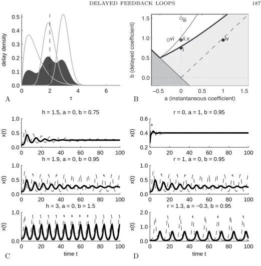
When f is not a Dirac mass, there is no such strict order on the branches. They can intersects at
several points, so that the boundary of the stability region will be determined by the first branch
crossed when moving continuously from the line a = b. For instance, when the delay distribution
takes three distinct discrete delay, at least the four first branches are needed to determine the
stability boundary (Figure
4.1
). The stability chart in the (a, b)-space then becomes a tangled
monster plot
1.
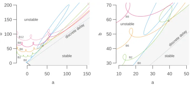
0 50 100 150 0 50 100 150 200 a b stable unstable discrete dela y B0 B2 B6 B8 B12 10 20 30 40 50 30 40 50 60 70 a b stable unstable discrete dela y B0 B2 B6 B8
Figure 4.1: Tangled monster plot (stability chart) for the characteristic equation with three discrete
delays λ + a + b
∑
3i=1p
iexp(−λτ
i) = 0, with τ =
{0.3731, 0.7090, 5.9701} and p = {0.7, 0.2, 0.1}.
The mean delay is s = 1. The stability region (grey area: stable) is located below the union of the
branches (colored curves: B
0, B
2, B
6, B
8, and B
12; the curves B
4and B
10are not visible on these
axes) on which the characteristic equation admits imaginary roots
±iω with increasing values of ω.
The stability boundary of the characteristic equation with a single delay at 1: λ+a+b exp(
−λ) = 0
lies entirely in the stable region (grey curve: discrete delay). The stability region with three delay
is bounded by a non-trivial union of parametric curves (enlarged in right panel). For instance, at
the point (a, b) = (39.5, 59) (point +), the characteristic equation in unstable, but only because
of branch B
6(orange).
4.2
G
⟨n⟩[dM]
The Goodwin model is perhaps the best-known model of a genetic oscillator. Introduced in the
1960’s by B. Goodwin [
35
], it describes the activity of a gene (mRNA expression x), its product
(protein concentration y) and the formation of a negative regulator complex z that inhibit gene
expression.
dx
dt
= P (z)
− αx,
dy
dt
= β[x
− y],
dz
dt
= β[y
− z],
where the nonlinear function P is a Hill function
P (z) = k
01
1 + z
h.
The parameters α, β, k
0, h
have all real, positive values. (The original Goodwin had different
co-efficients for each dynamical variable, but we keep things simple.) Parameter α is the mRNA
degradation rate, β is the degradation rate of the protein products, k
0is the maximal mRNA
syn-thesis rate. Parameter h is the Hill coefficient. There are parameters for which the Goodwin
model has unique, unstable, positive equilibrium, and a stable, positive limit cycle. However, the
limit cycle exists only for relatively large values of the Hill coefficient, h > 8. There are several
ways to modify the Goodwin model so that solutions will oscillate more easily. The reason the
4.3. STABILITY RESULTS
23
Goodwin model can oscillate is that it is a system with a delayed, negative feedback loop. The loop
is clear: x depends on z, which depends on x. It is negative because P is a decreasing function,
and it is delayed because z is a delayed version of x. We can increase the length of the delay by
adding more intermediary steps between x and z, i.e. by replacing y and z with y
1, y
2, ..., y
qand
defining the corresponding ODEs
dy
idt
= β(y
i−1− y
i), i = 1, ..., q,
where, for ease of notation, y
0= x
and y
q= z.
I became interested in the Goodwin oscillator in 2004 while I was working with Hanspeter Herzel
at the Institute for Theoretical Biology in Berlin. There I met Didier Gonze, who was studying how
circadian clocks could synchronize to form a pacemaker. The Goodwin model had been applied
to the circadian clock already [
56
], and it seemed like a good compromise between the realism of
complexity and the simplicity of abstraction. Robust synchronization of nonlinear oscillators is
far from trivial, and we tried several versions of the Goodwin models as a core circadian oscillator
with varying degree of success. To keep up with these different model versions, we developed a
naming convention. We called the Goodwin model with one nonlinear equation and q auxiliary
linear equations
G⟨q + 1⟩. Under this naming convention, the original Goodwin model is
G3. It
is the smallest model that admits a stable limit cycle. Model
G2has only one auxiliary equation,
and it is a classical result that no such 2-dimensional negative feedback system can admit a limit
cycle. In general, the larger the q, the easier it is to produce stable limit cycles. In the limit q
→ ∞
(while q/β
→ τ > 0), the Goodwin model becomes a scalar equation with a discrete delay
dx
dt
= P (x
s)
− αx,
(4.4)
where x
s= x(t
− s). This model is denoted
G1d(
dfor delay), and is equivalent to
G∞.
Another way to modify the Goodwin model is to replace linear degradation term with nonlinear
ones. We used in [
34
] a modified version of the Goodwin model where the degradation terms
followed Michaelis-Menten kinetics,
v
x
K + x
.
(4.5)
These models are denoted
G⟨n⟩
Mfollowed optionally with the indices of the variable for which
the degradation rate is nonlinear. Introduction of nonlinear degradation rates helps producing
sustained oscillations, but care must be taken to make sure solutions do not blow up.
4.3
Stability results
A Goodwin model
G⟨n⟩ possesses exactly one positive equilibrium, given by the unique positive
solution of P (x)
− αx = 0. Its asymptotic stability is determined by a characteristic polynomial
of degree n = q + 1. In practice, the roots can be inconvenient to locate, especially when n is large
[
18
]. To avoid dealing with cumbersome high degree polynomials, we can use the linear chain
trick to convert the system
G⟨n⟩ into a scalar differential with a distributed delay. The linear chain
trick consists in integrating the auxiliary variables y
isuccessively, keeping the dependence on x.
This way z can be expressed as a linear functional on the history of x:
z(t) =
∫
∞0
where g is the Gamma distribution
g(τ, q, β) =
β
q
Γ(q)
τ
q−1
e
−βτ.
(4.7)
The mean delay s = q/β. Model
G⟨n⟩ can then be expressed as
dx
dt
= P (z)
− αx,
(4.8)
with z defined by equation (
4.6
). We note that q, the number of auxiliary equations, is now a
ordinary parameter that can take any non-negative real value.
Let ¯
x
be the unique positive equilibrium of equation (
4.8
), then the characteristic equation of the
linear system at equilibrium is
λ + a + b
∫
∞0
g(τ, q, β)e
λτdτ = 0.
(4.9)
Coefficients are a = α and b =
−dP /dx|
x¯≥ 0. For q ∈ N, the characteristic equation has the same
n
roots as the characteristic polynomial, so no advantage can be gained analytically with the linear
chain trick. The roots of the characteristic equation determine the asymptotic stability of the
equilibrium ¯
x. The equilibrium is asymptotically stable if and only if all roots have strictly negative
real parts. However, we know how the roots of the characteristic equation behave when q goes to
infinity, while q/β
→ s. By continuity, the roots of the characteristic equation will converge to the
roots of the characteristic equation associated to the model
G1d. The characteristic equation for
model
G1dis
λ + a + be
−λs= 0.
(4.10)
All roots of the equation (
4.10
) have strictly negative real parts if one of the conditions is
satis-fied
1. a
≥ |b| and a > −b,
2. b > a and
s <
arccos(
√
−a/b)
b
2− a
2.
(4.11)
If none of the conditions are satisfied, there is at least one root with nonnegative real part. Our
main stability result [
16
, Article in Section
9.1
] generalizes previous results [
18
]. It states that if
either of the above conditions is satisfied, all roots of the characteristic equation (
4.9
) for model
G
⟨n⟩ also have strictly negative real parts. This stability results holds not only for delay equations
with Gamma distributions, but for any distribution with at least an exponential tail. These
suffi-cient conditions are also necessary when the distribution is a single discrete delay. Our stability
results are optimal in the sense that if the stability conditions are not met, we can find a delay
distribution with mean s such that the corresponding characteristic equation will possess a root
with a nonnegative real part. Put another way, replacing a discrete delay by a distribution of delay
cannot destabilize an equilibrium.
In practice, the bound defined by inequality (
4.11
) is quite conservative. Wide delay distributions
tend to expand the region of stability in the (a, b)-space at s fixed. In Figure
4.1
, the shaded area
(stable) above the grey curve (discrete delay) is the region in the (a, b)-space that is stable for
the distributed delay, but unstable for the single delay. For instance, at a = 30, the stability
region is extended from b
≈ 30 to b ≈ 40. Despite the conservative conditions on a, b and s for
stability, there are obvious advantages to be able to draw stability conclusions based only on three
parameters: the coefficients a, b and the first moment of the distribution s.
4.4. POSITIVE FEEDBACK LOOPS AND ROBUSTNESS OF OSCILLATIONS
25
4.4
Positive feedback loops and robustness of oscillations
The Goodwin model and its variants have been used to model anything from small gene
regu-latory networks involving Hes1, p53, and NF-κB [
50
] (
G2d), or the circadian clock [
56
] (
G3), to
cell populations with density-dependent growth rates, as exemplified by a model for erythrocyte
production [
10
] (
G1d).
We have identified the ingredients needed to obtain oscillations in terms of the characteristic
equation: a strong negative feedback loop b >
|a|, and a significant delays. If the delay is
dis-crete, then for any a
≥ 0, there will be a critical value b for which a pair of complex roots of the
characteristic equation will cross the imaginary axis. The Hopf bifurcation theorem states that
(generically) a small amplitude limit cycle appears right there. There are often objections as to
whether the negative-feedback+delay combo is sufficient for oscillations in real genetic oscillators
and populations. The strength of the feedback is mostly determined by the Hill coefficient, and
only very specific mechanisms can produce values much larger than 4 [
65
]. Moreover, the delay
is likely to be smooth rather than “spiky”, and this increases the region of stability. Our stability
results tend to support these arguments that in practice it may be difficult to achieve a delay large
enough to make sustained oscillations possible.
How can biological oscillators be robust then? It has been suggested that adding positive feedback
could make an oscillator more robust [
2
,
63
]. A simple positive feedback loop can be incorporated
by slightly modifying the nonlinear term
P (x, z) = k
0x
r1 + z
h.
The coefficient r is a cooperativity coefficient. When r < 1, cooperativity is negative, and the
positive feedback is most active for small values of x. When r > 1, cooperativity is positive, and
the loop is active for large values of x. When r = 1, cooperativity is neutral. The introduction
of a positive feedback loop can easily destabilize even a system that could never oscillate. This
happens because positive feedback loops shifts the parameter a to the left. Therefore, for any
b
≥ s
−1there will always be a value of a >
−b, such that the characteristic equation has a pair of
imaginary roots, and destabilization will occur through a Hopf bifurcation.
For instance, the characteristic equation for the model
G2with a positive feedback loop is
λ + α(1
− r) +
α
2h
k
0¯
x
h−r+1∫
∞ 0e
−λτβe
−βτdτ = 0.
The integral term simplifies to β/(λ + β), and the characteristic equation reduces to the familiar
second-order polynomial
λ
2+
(
β + α(1
− r)
)
λ +
α
2h
k
0¯
x
h−r+1+ αβ(1
− r) = 0.
We are looking for a pair of complex roots with positive real part. When r = 0, the case without
positive feedback loop, the roots cannot be complex and have a positive real part, since the trace
−α − β is negative. Another way to see that is that the characteristic equation possesses only one
branch of imaginary roots for b >
|a|, which is exactly the line
(
a =
−s
−1, b > s
−1)
. Because
a = α > 0
the stability boundary cannot be reached.
When r > 1, however, the trace α(r
− 1) − β can be positive. At the same time, parameters k
0and
h
can be chosen as to have a negative discriminant. Therefore, positive instantaneous feedback
loops with positive cooperativity can destabilize stable fixed points through a Hopf bifurcation.
As a rule of thumb, we can assume that increasing the cooperativity r has a destabilizing effect:
−2.0
−1.5
−1.0
−0.5
0.0
0.5
1.0
1.5
2.0
2.5
3.0
3.5
a
b
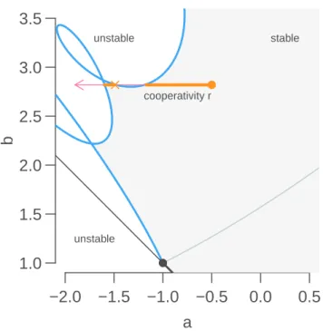
stable unstable unstable cooperativity rFigure 4.2: Tangled monster plot (stability chart) for the characteristic equation with three
discrete delays with characteristic equation λ + α(1
− r) + b
∑
3i=1p
iexp(−λτ
i) = 0, with
τ =
{0.3731, 0.7090, 5.9701} and p = {0.7, 0.2, 0.1} (delay parameters as in Figure
4.1
, and
a = α(1
−r)). Increasing the cooperativity coefficient r while keeping b constant always eventually
destabilizes a steady state, but stability switches can occur (×).
the real part of the leading eigenvalues of the characteristic equation increases with r. This is
not always true, because stability switches can occur, as evidence by a close up on the tangled
monster plots (Figure
4.2
).
The main limitation of the sufficient condition for stability is that it cannot handle mixed delayed
feedback loops, i.e. loops with negative and positive delayed components. What happens when
the positive feedback loop is delayed is a bit more complicated. Intuitively, a positive loop with
a sufficiently large delay should be destabilizing. The characteristic equation of the scalar mixed
feedback loop equation would be
λ + a + be
λτ1− ce
λτ2= 0,
assuming bc > 0. This characteristic equation has been studied from different angles [
36
,
46
,
24
,
55
]. We have recently obtained promising results concerning the locations of the roots (A Besse,
2017, Ph.D. thesis in preparation). Briefly, for τ
1fixed, and c not too large, there is a smooth curve
B
in partitioning the region b
≥ | − a + c| such that
1. If b < B, for any τ
2≥ 0, all roots have negative real parts.
2. If b > B, there exists τ
2≥ 0 such that the leading roots have positive real parts.
The inequality b < B is to be understood by the existence of ¯b > b such that
(
a, ¯
b
)
∈ B, and
b > B
if there is no such value. This curve B is the “lower” part of the envelope of the limit set
of the parametric curve B
0(and only B
0) when τ
2→ ∞. This result should be generalizable
to delay distributions, where the curve B would be optimal when the negative feedback delay is
discrete.
Chapter 5
Synchronization and rhythmicity of
circadian clocks
5.1
The circadian clock
The circadian clock is a biological clock that controls daily rhythms in physiology and behavior.
In mammals it is controlled by a pacemaker located in the suprachiasmatic nucleus (SCN) of the
hypothalamus. In mice, the SCN is composed of 20,000 densely packed neurons. Each of these
neurons possesses a gene regulatory network with interlocked positive and negative feedback
loops that can generate 24 hour-period oscillations in molecular concentrations. Neurons in the
SCN are organized in different regions, characterized by which neuropeptides or
neurotransmit-ters they express and whether they can receive direct light input from the retina. The ventrolateral
part of the SCN receives light from the retina and relays the information to the dorsomedial part.
As a whole, the SCN is capable of producing a coherent daily rhythm. The disparate intracellular
clocks form a coherent rhythm through mutual interaction, or coupling.
It was initially observed that neurons dispersed in cell culture mostly displayed cell-autonomous
oscillations [
66
], but a more recent study showed that when neurons are dispersed at a lower
density, most neurons display no or irregular oscillations [
64
]. When key circadian clock genes are
knocked-out, making isolated cells arrhythmic, animal behavior can still be rhythmic, indicating
that cell-cell interaction can rescue oscillations [
45
,
39
].
So, based on available experimental data, we were looking for mechanisms to synchronize
self-sustained oscillators. However, from a mathematical point of view, damped oscillators would be
more appropriate. Damped oscillators can be entrained at any frequency, while entrainment of
sustained oscillators can show complex periodic and non-periodic solutions.
5.2
Damped versus sustained oscillators
The idea that circadian rhythms could be generated by mutually coupled damped oscillators was
already proposed by Enright in the 1980’s [
30
]. Enright used mutually triggered damped, noisy
relaxation oscillators, interconnected in such a way that when a given fraction of elements have
fire up, all connected elements are triggered and reset to phase 0. Enright defines a damped
relaxation oscillator so that when isolated, it will fire with an amplitude 1 at the first cycle, k < 1
at the second cycle, k
2at the third cycle, and so on. Amplitude is reset to 1 when the oscillator is
reset. It is intuitively clear such oscillators can become sustained through mutual entrainment, as
soon as enough oscillators fire at each cycle. Enright’s model shows how unreliable oscillators can
produce a reliable timekeeping. However, the assumption that individual clocks can be modeled
as relaxation oscillator is a strong one. Relaxation oscillators arise at short biological time scales.
For instance in neuron action potentials or pancreatic beta cell insulin secretion occur at a time
scales of milliseconds to minutes. It is not clear how much slower cycles, from circadian clocks
to menstrual cycles can be considered as relaxation oscillators. Relaxation oscillators, with a
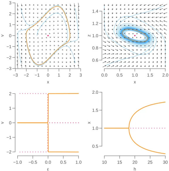
fast-slow dynamics, such as the van der Pol oscillator, tend to have an all-or-none dynamics (Figure
5.1
, left panels). The van der Pol oscillator is a non-linearly (negatively) damped oscillator
¨
x
− εω
0(1
− x
2) ˙
x + ω
02x = 0.
The damping coefficient
−εω
0(1
− x
2)
is negative for small values of
|x| and positive values of
ε
(assuming ω
0> 0), and negative for larger values of
|x|. Poincaré-Bendixson theorem can be
applied to show that the van der Pol oscillator admits a stable limit cycle.
Several experimental reports suggested that cellular clocks have sustained sinusoidal oscillations,
even in isolated cells [
66
,
51
]. Multiple genetic regulation feedback loops, both positive and
tive, have been identified, but the experimental and theoretical consensus is that a delayed
nega-tive loop is sufficient to generate and maintain a 24h cycle in molecular levels [
53
]. The Goodwin
5.2. DAMPED VERSUS SUSTAINED OSCILLATORS
29
−3 −2 −1 0 1 2 3 −3 −2 −1 0 1 2 3 x v 0.0 0.5 1.0 1.5 2.0 0.6 0.8 1.0 1.2 1.4 x z −1.0 −0.5 0.0 0.5 1.0 −2 −1 0 1 2 ε v 10 15 20 25 30 0.5 1.0 1.5 2.0 h xFigure 5.1: Van der Pol (top left, ε = 1, ω
0= 1) and
G3(top right, β = 1, α = 1, k
0= 2, h = 20)
phase spaces. The phase space of
G3has been projected onto the xz-plane, for y interpolated from
numerical solution: for (x, z), y was set to y(t), where
||(x, z) − (x(t), z(t))|| is minimized along
all times t. Bifurcation diagrams of the van der Pol oscillator with respect to ε (bottom left) and
G3
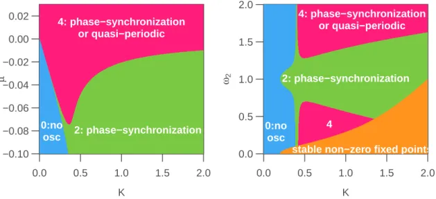
![Figure 5.3: Synchronization of N = 100 globally-coupled (coupling matrix is one) non-identical oscillators with coupling strength K = 0.4, random frequencies ω ∼ U [0.8, 1.2] and µ = 0.08 (orange, sustained oscillators), µ = − 0.08 (blue, damped oscillator](https://thumb-eu.123doks.com/thumbv2/123doknet/14702754.747323/39.892.128.732.126.407/synchronization-globally-identical-oscillators-frequencies-sustained-oscillators-oscillator.webp)


![Figure 6.2: Atmospheric 14C profiles for different turnover rates. The atmospheric 14C levels be- be-tween shows a steep rising phase bebe-tween 1955 and 1963, and a slow decrease since then [44]](https://thumb-eu.123doks.com/thumbv2/123doknet/14702754.747323/48.892.231.652.128.508/figure-atmospheric-profiles-different-turnover-atmospheric-levels-decrease.webp)