HAL Id: hal-00426502
https://hal.archives-ouvertes.fr/hal-00426502
Submitted on 26 Oct 2009HAL is a multi-disciplinary open access archive for the deposit and dissemination of sci-entific research documents, whether they are pub-lished or not. The documents may come from teaching and research institutions in France or
L’archive ouverte pluridisciplinaire HAL, est destinée au dépôt et à la diffusion de documents scientifiques de niveau recherche, publiés ou non, émanant des établissements d’enseignement et de recherche français ou étrangers, des laboratoires
On the Moments of the Aggregate Discounted Claims
with Dependence Introduced by a FGM Copula
Mathieu Bargès, Hélène Cossette, Stéphane Loisel, Etienne Marceau
To cite this version:
Mathieu Bargès, Hélène Cossette, Stéphane Loisel, Etienne Marceau. On the Moments of the Aggre-gate Discounted Claims with Dependence Introduced by a FGM Copula. ASTIN Bulletin, Cambridge University Press (CUP), 2011, 41 (1), pp.215-238. �hal-00426502�
On the Moments of the Aggregate Discounted Claims with
Dependence Introduced by a FGM Copula
Mathieu Barg`es∗‡ H´el`ene Cossette‡ St´ephane Loisel∗ Etienne Marceau´ ‡
October 22, 2009
Abstract
In this paper, we investigate the computation of the moments of the compound Poisson sums with discounted claims when introducing dependence between the interclaim time and the subsequent claim size. The dependence structure between the two random variables is defined by a Farlie-Gumbel-Morgenstern copula. Assuming that the claim distribution has finite moments, we give expressions for the first and the second moments and then we obtain a general formula for any mth order moment. The results are illustrated with applications to premium calculation, moment matching methods, as well as inflation stress scenarios in Solvency II.
Keywords : Compound Poisson process, Discounted aggregate claims, Moments, FGM copula, Constant interest rate.
1
Introduction
We consider a continuous-time compound renewal risk model for an insurance portfolio and we define the compound process of the discounted claims Xi, i = 1, 2, ... occurring at time Ti, i = 1, 2, ...
by Z ={Z (t) , t ≥ 0} with
Z (t) =
{ ∑N (t)
i=1 e−δTiXi, N (t) > 0
0, N (t) = 0,
where N = {N (t) , t ≥ 0} is an homogeneous Poisson counting process and δ the constant net interest rate. In actuarial risk theory, it is assumed that the claim amounts Xi, i = 1, 2, ... are
independent and identically distributed (i.i.d.) random variables (r.v.’s) and the interclaim times W1= T1 and Wj = Tj− Tj−1, j = 2, 3, ... are also i.i.d. r.v.’s. The r.v.’s Xi′ and Wi, i = 1, 2, ... are
∗Universit´e de Lyon, Universit´e Claude Bernard Lyon 1, Institut de Science Financi`ere et d’Assurances, 50 Avenue
Tony Garnier, F-69007 Lyon, France
classically supposed independent. This last assumption also implies that Xi, i = 1, 2, ... are
indepen-dent from N . This risk process has been used in ruin theory by many authors such asTaylor(1979),
Waters (1983), Delbaen and Haezendonck (1987), Willmot(1989), Sundt and Teugels (1995) and more recently Kalashnikov and Konstantinides (2000), Yang and Zhang (2001) and Tang (2005). They mainly focused on the ruin probability and related ruin measures.
Only a few recent works deal with the distribution of the aggregate discounted claims Z(t).
L´eveill´e and Garrido(2001a) provide the first two moments of this process. These first two moments were also obtained in Jang (2004) using martingale theory. This result has since been generalized by relaxing some of the classical assumptions presented above. L´eveill´e and Garrido (2001b) and
L´eveill´e et al. (2009) derived recursive formulas for all the moments of the aggregate discounted claims considering a compound renewal process where N is not necessarily a Poisson process. In Jang (2007), the Laplace transform of the distribution of a jump diffusion process and its integrated process is derived and used to obtain the moments of the compound Poisson process Z(t). Kim and Kim(2007) andRen(2008) studied the discounted aggregate claims in a Markovian environment which modulates the distributions of the interclaim times and claim sizes for the former and the distribution of the interclaim times for the latter. They both provided the Laplace transform of the distribution of the discounted aggregate claims and then gave expressions for its first two moments.
The aggregation of discounted random variables is also used in many other fields of application. For example, it can be used in warranty cost modeling, see Duchesne and Marri (2009), or in reliability in civil engineering, seevan Noortwijk and Frangopol (2004) or Porter et al.(2004).
In this paper, we want to introduce some dependence between the interclaim times and the sub-sequent claim amounts. In risk theory, this dependence has already been explored. For example,
Albrecher and Boxma (2004) supposed that if a claim amount exceeds a certain threshold, then the parameters of the distribution of the next interclaim time is modified. InAlbrecher and Teugels
(2006) the dependence is introduced with the use of an arbitrary copula. Conversely toAlbrecher and Boxma
(2004),Boudreault et al.(2006) assumed that if an interclaim time is greater than a certain thresh-old then the parameters of the distribution of the next claim amount is modified. In a similar dependence model, but with more freedom in the choice of the copula between each interclaim time and the subsequent claim amount, Asimit and Badescu(2009) consider a constant force of interest and heavy-tailed claim amounts. Dependence concepts used inBoudreault et al.(2006) were then extended in Biard et al. (2009) where they suppose that the distribution of a claim amount has its parameters modified when several preceding interclaim times are all greater or all lower than a certain threshold. All these papers were interested in finding exact expressions or approximations for some ruin measures such as the ruin probability or the Gerber-Shiu function.
In our study, this assumption of independence between the claim amount Xj and the
inter-claim time Wj is relaxed to allow {(Xj, Wj) , j∈ N+} to form a sequence of i.i.d. random vectors
distributed as the canonical random vector (X, W ) in which the components may be dependent. We follow the idea of Albrecher and Teugels(2006) supposing that dependence is introduced by a copula between an interclaim time and its subsequent claim amount. More specifically, we use the Farlie-Gumbel-Morgenstern (FGM) copula which is defined by
for (u, v)∈ [0, 1] × [0, 1] and where the dependence parameter θ takes value in [−1, 1]. While there are a large number of copula families, we choose the FGM copula because it offers the advantage of being mathematically tractable as it is illustrated in Cossette et al. (2009). Even if the FGM copula introduces only light dependence, it admits positive as well as negative dependence between a set of random variables and includes the independence copula when θ = 0. It is also known that the FGM copula is a Taylor approximation of order one of the Frank copula (see Nelsen (2006), page 133), Ali-Milkhail-Haq copula and Plackett copula (see Nelsen(2006), page 100).
The paper is structured as follows. In the second section, we present the model of the continuous time compound Poisson risk process that we use and give some notation. The first moment, the second moment and then a generalization to the mth moment are derived in Section 2. Applications to premium calculation, moment matching methods and Solvency II are given in the third section. In particular, we show how our method may be used to determine Solvency Capital Requirements and to perform part of Own Risk and Solvency Assessment (ORSA) analysis in Solvency II for some cat risks and inflation risk.
2
The model
As explained in the introduction, we consider the continuous-time compound Poisson process Z = {Z (t) , t ≥ 0} of the discounted claims X1, ..., XN (t) occurring at times T1, ..., TN (t) with
Z (t) =
{ ∑N (t)
i=1 e−δTiXi, N (t) > 0
0, N (t) = 0, where E[Xik] <∞ for i = 1, 2, ...
We introduce a specific structure of dependence based on the Farlie-Gumbel-Morgenstern copula between the ith claim amount and the ith interclaim time such that, using (1), the joint cumulative distribution function (c.d.f.) for the canonical random vector (X, W ) is
FX,W(x, t) = C (FX(x) , FW(t))
= FX(x) FW(t) + θFX(x) FW(t) (1− FX(x)) (1− FW (t)) ,
for (t, x) ∈ R+ × R+ and where FX and FW are the marginals of respectively X and W . This
dependence relation implies that X1, X2, X3, ... are no more independent of N . Recalling the density of the FGM copula
cF GMθ (u, v) = 1 + θ (1− 2u) (1 − 2v) ,
for (u, v)∈ [0, 1] × [0, 1], the joint probability density function (p.d.f.) of (X, W ) is fX,W (x, t) = cF GMθ (FX(x) , FW(t)) fX(x) fW (t)
= fX(x) fW (t) + θfX(x) fW(t) (1− 2FX(x)) (1− 2FW(t)) ,
The mth moment of Z (t) is denoted by µ(m)Z (t) = E[Z(m)(t)] and its Laplace transform by eµ(m)
Z (r) with m∈ R+. We see in the next section how to derive explicit formulas for these moments.
3
Moments of the aggregate discounted claims
3.1 First moment
To derive the expression for the first moment µZ(t) of Z(t), we condition on the arrival of the first
claim µZ(t) = E [Z (t)] = E [ E [ e−δsX1+ e−δsZ(t− s)|W1 = s ]] = ∫ t 0 fW(s) e−δsE [X|W = s] ds + ∫ t 0 fW (s) e−δsµZ(t− s) ds, where E [X|W = s] = ∫ ∞ 0 xfX|W =s(x) dx = ∫ ∞ 0 x{(1 + θ (1 − 2FX(x)) (1− 2FW(s)))} fX(x) dx = E [X] + θ ∫ ∞ 0 x (2− 2FX(x)) (1− 2FW(s)) fX(x) dx −θ ∫ ∞ 0 x (1− 2FW(s)) fX(x) dx = E [X] (1− θ (1 − 2FW(s))) +θ (1− 2FW(s)) ∫ ∞ 0 (1− FX(x))2dx. (2) Letting E[X′]= ∫ ∞ 0 (1− FX(x))2dx < ∫ ∞ 0 (1− FX(x)) dx = E [X] , (2) becomes E [X] +(E[X′]− E [X])θ (1− 2FW (s)) . (3)
From (3), we can derive the following remarks. If θ > 0 (θ < 0) and s < FW−1(0.5) (s > FW−1(0.5), respectively), then E [X|W = s] < E [X]. Conversely, if θ > 0 (θ < 0) and s > FW−1(0.5) (s < FW−1(0.5), respectively), then E [X|W = s] > E [X] .
and fW(t) = βe−βt, (4) FW(t) = 1− e−βt, (5) e fW(s) = E [ e−sW]= β β + s.
For simplification purposes, we use the expressions h (s; γ) = γe−γs bh (r; γ) = γ
γ + r to derive the moments of Z(t).
We obtain the following expression for µZ(t)
µZ(t) = ∫ t 0 fW (s) e−δsE [X] ds + θ ( E[X′]− E [X]) ∫ t 0 fW(s) e−δs(1− 2FW(s)) ds + ∫ t 0 fW(s) e−δsµZ(t− s) ds = ∫ t 0 βe−βse−δsE [X] ds + θ(E[X′]− E [X]) ∫ t 0 βe−βse−δs ( 2e−βs− 1 ) ds + ∫ t 0 βe−βse−δsµZ(t− s) ds = ∫ t 0 β β + δh (s; β + δ) E [X] ds +θ(E[X′]− E [X]) ∫ t 0 2β 2β + δh (s; 2β + δ) ds −θ(E[X′]− E [X]) ∫ t 0 β β + δh (s; β + δ) ds + ∫ t 0 β β + δh (s; β + δ) µZ(t− s) ds. (6)
We take the Laplace transform on both sides of (6) and after some rearrangements, we obtain
eµZ(r) = bh(r;β+δ) r β β+δE [X] + θ (E [X′]− E [X]) ( 2β 2β+δ bh(r;β+δ) r − β β+δ bh(r;β+δ) r ) 1−β+δβ bh (r; β + δ) (7) which is equivalent to eµZ(r) = 1 r β+δ β+δ+r β β+δE [X] + θ (E [X′]− E [X]) ( 2β 2β+δ 1 r 2β+δ 2β+δ+r− β β+δ 1 r β+δ β+δ+r ) 1−β+δβ β+δ+rβ+δ . (8)
Rearranging (8), we deduce eµZ(r) = βE[X] r(δ + r) + θ β (E[X′]− E[X]) r(2β + δ + r) . (9) Inverting (9), we obtain µZ(t) = βE[X] 1− e−δt δ + θβ ( E[X′]− E[X]) 1 − e −(2β+δ)t 2β + δ . (10)
Notice that when the r.v.’s X and W are independent which corresponds to θ = 0, the expected value of the compound process of the discounted claims, noted Zind(t), becomes
µZind(t) = βE[X]
1− e−δt
δ .
3.2 Second moment
As for the first moment of the discounted total claim amount, we condition on the arrival of the first claim to obtain the second moment of Z(t)
µ(2)Z (t) = E [ E [ (e−δsX1+ e−δsZ(t− s))2|W1 = s ]] = ∫ t 0 fW(s) e−2δsE [ X2|W = s]ds + 2 ∫ t 0 fW (s) e−2δsE [X|W = s] µZ(t− s) ds + ∫ t 0 fW(s) e−2δsµ(2)Z (t− s) ds. Similarly as in (2), we have E[X2|W = s] = E[X2](1− θ (1 − 2FW(s))) +θ (1− 2FW(s)) ∫ ∞ 0 2x (1− FX(x))2dx = E[X2]+ ( E [( X′ )2] − E[X2])θ (1− 2FW(s)) , where E[(X′)2 ] = ∫ ∞ 0 2x (1− FX(x))2dx < ∫ ∞ 0 2x (1− FX(x)) dx = E [ X2].
We find the following expression for µ(2)Z (t) µ(2)Z (t) = ∫ t 0 fW(s) e−2δsE [ X2]ds + θ ( E[(X′)2 ] − E[X2]) ∫ t 0 fW(s) e−2δs(1− 2FW(s)) ds +2 ∫ t 0 fW(s) e−2δsE [X] µZ(t− s) dsds +2θ(E[(X′)]− E [X]) ∫ t 0 fW(s) e−2δs(1− 2FW(s)) µZ(t− s) ds + ∫ t 0 fW(s) e−2δsµ(2)Z (t− s) ds = ∫ t 0 β β + 2δh (s; β + 2δ) E [ X2]ds +θ ( E[(X′)2 ] − E[X2]) ∫ t 0 ( 2β 2β + 2δh (s; 2β + 2δ)− β β + 2δh (s; β + 2δ) ) ds +2 ∫ t 0 β β + 2δh (s; β + 2δ) E [X] µZ(t− s) ds +2θ(E[(X′)]− E [X]) ∫ t 0 ( 2β 2β + 2δh (s; 2β + 2δ)− β β + 2δh (s; β + 2δ) ) µZ(t− s) ds + ∫ t 0 β β + 2δh (s; β + 2δ) µ (2) Z (t− s) ds. (11)
We take the Laplace transform on both sides of (11) and after some rearrangements, we obtain
˜ µ(2)Z (r) = 1 1−β+2δβ bh(r; β + 2δ) [ bh(r; β + 2δ) r β β + 2δE[X 2] +θ(E[(X′2]− E[X2]) ( 2β 2β + 2δ bh(r; 2β + 2δ) r − β β + 2δ bh(r; β + 2δ) r ) +2E[X] β β + 2δbh(r; β + 2δ)˜µZ(r) +2θ(E[X′]− E[X]) ( 2β 2β + 2δ ˆ h(r; 2β + 2δ)− β β + 2δbh(r; β + 2δ) ) ˜ µZ(r) ] , which becomes ˜ µ(2)Z (r) = βE[X 2] r(2δ + r) + θ β(E[(X′2]− E[X2]) r(2β + 2δ + r) + 2 βE[X] 2δ + rµ˜Z(r) + 2θ β (E[X′]− E[X]) 2β + 2δ + r µ˜Z(r) = βE[X 2] r(2δ + r) + θ β(E[(X′2]− E[X2]) r(2β + 2δ + r) + 2 βE[X] 2δ + r ( βE[X] r(δ + r) + θ β (E[X′]− E[X]) r(2β + δ + r) ) +2θβ (E[X ′]− E[X]) 2β + 2δ + r ( βE[X] r(δ + r) + θ β (E[X′]− E[X]) r(2β + δ + r) ) = βE[X 2] r(2δ + r) + θ β(E[(X′2]− E[X2]) r(2β + 2δ + r) + 2 β2E[X]2 r(δ + r)(2δ + r)+ 2θ β2E[X] (E [X′]− E[X]) r(2β + δ + r)(2δ + r) +2θβ 2E[X] (E [X′]− E[X]) r(δ + r)(2β + 2δ + r) + 2θ 2 β2(E [X′]− E[X]) 2 r(2β + δ + r)(2β + 2δ + r). (12)
This last Laplace transform is a combination of terms of the form ˜
f (r) = 1
r(α1+ r)(α2+ r)...(αn+ r)
,
with f a function defined for all non-negative real numbers. As described in the proof of Theorem 1.1 in Baeumer (2003), each of these terms can be expressed as a combination of partial fractions such as ˜ f (r) = γ0 1 r + γ1 1 α1+ r + γ2 1 α2+ r + ... + γn 1 αn+ r , (13)
where γ0 = α1...α1 n and , for i = 1, ..., n,
γi =− 1 αi n ∏ j=1;j̸=i 1 αj− αi . (14)
Since the inverse Laplace transform of α1 i+r is e
−αit, it is easy to inverse ˜f and obtain
f (t) = γ0+ γ1e−α1t+ γ2e−α2t+ ... + γne−α2t. (15)
Using (15) in (12), it results that
µ(2)(t) = βE[X2] ( 1 2δ − e−2δt 2δ ) + θβ(E[(X′2]− E[X2]) ( 1 2β + 2δ − e−(2β+2δ)t 2β + 2δ ) +2β2E[X]2 ( 1 2δ2 − e−δt δ2 + e−2δt 2δ2 )
+2θβ2E[X](E[X′]− E[X]) ( 1 2δ(2β + δ) − e−(2β+δ)t (2β + δ)(−2β + δ) + e−2δt 2δ(−2β + δ) )
+2θβ2E[X](E[X′]− E[X]) ( 1 δ(2β + 2δ) − e−δt δ(2β + δ)+ e−(2β+2δ)t (2β + 2δ)(2β + δ) ) +2θ2β2(E[X′]− E[X])2 ( 1 (2β + δ)(2β + 2δ)− e−(2β+δ)t δ(2β + δ) + e−(2β+2δ) δ(2β + 2δ) ) . (16)
3.3 mth moment
We now generalize the previous results to the mth moment of the discounted total claim amount. Conditioning on the arrival of the first claim leads to
µ(m)Z (t) = ∫ t 0 fW (s) e−mδsE [Xm|W = s] ds + m∑−1 j=1 ( m j ) ∫ t 0 fW (s) e−mδsE [ Xj|W = s]µ(mZ −j)(t− s) ds + ∫ t 0 fW(s) e−mδsµ(m)Z (t− s) ds.
For the Laplace transform of µ(m)Z (t), we find eµ(m) Z (r) = 1 1−β+mδβ bh (r; β + mδ) [ bh (r; β + mδ) r β β + mδE [X m] +θ(E[(X′)m]− E [Xm]) ( 2β 2β + mδ bh (r; 2β + mδ) r − β β + mδ bh (r; β + mδ) r ) + m∑−1 j=1 ( m j ) E[Xj] β β + mδbh (r; β + mδ) eµ (m−j) Z (r) + θ m∑−1 j=1 ( m j ) ( E[(X′)j ] − E[Xj]) × ( 2β 2β + mδbh (r; 2β + mδ) − β β + mδbh (r; β + mδ) ) eµ(m−j) Z (r) ] (17)
which can also be expressed as follows
˜ µ(m)Z (r) = ( m m ) βE[Xm] r(mδ + r) + ( m m ) θβ (E [(X ′m]− E[Xm]) r(2β + mδ + r) + m∑−1 j=1 ( m j ) βE[Xj] mδ + rµ˜ (m−j) Z (r) +θ m∑−1 j=1 ( m j ) β(E[(X′j]− E[Xj]) 2β + mδ + r µ˜ (m−j) Z (r).
Noting for i = 1, ..., m, j = 1, ..., m and k = 0, 1
ζ(i; j; k) = ( i j ) θkβ (
E[Xj])1−k(E[X′j]− E[Xj])k k× 2β + iδ + r =
Λ(i; j; k)
k× 2β + iδ + r, (18) we can rewrite ˜µZ(r) and ˜µ(2)Z (r) as
˜ µZ(r) = 1 r [ ζ(1, 1, 0) + ζ(1, 1, 1) ] ,
˜ µ(2)Z (r) = 1 r [ ζ(2, 2, 0) + ζ(2, 2, 1) + [ζ(2, 1, 0) + ζ(2, 1, 1)] [ζ(1, 1, 0) + ζ(1, 1, 1)] ] = 1 r [ ζ(2, 2, 0) + ζ(2, 2, 1) + ζ(2, 1, 0)ζ(1, 1, 0) + ζ(2, 1, 0)ζ(1, 1, 1) + ζ(2, 1, 1)ζ(1, 1, 0) +ζ(2, 1, 1)ζ(1, 1, 1) ] .
The term ˜µ(m)Z (r) can also be expressed using (18)
˜ µ(m)Z (r) = 1 r m ∑ n=1 ∑
((i1,j1,k1),...,(in,jn,kn))∈Amn
ζ(in, jn, kn)× ... × ζ(i1, j1, k1), (19) where Amn = { (i1, j1, k1), ..., (in, jn, kn); i1 = m, i1+...+in= m−1+n, i1 > ... > in, j1 = m+1−n, j1+ ... + jn= m, j1 ≥ ... ≥ jn, k.∈ {0, 1} } .
To inverse (19), let I (ζ(i1; j1; k1); ...; ζ(in; jn; kn)) be the inverse Laplace transform of1rζ(i1; j1; k1)×
...× ζ(in; jn; kn), for n = 1, ..., m. Using (13) and (15), we have
I (ζ(i1; j1; k1); ...; ζ(in; jn; kn)) = Λ(i1; j1; k1)×...×Λ(in; jn; kn)×
(
γ0+ γ1e−α(i1;k1)t+ ... + γne−α(in;kn)t
)
with, refering to (14), γ0 = α(i 1
1;k1)...α(in;kn) and γu = − 1
α(iu;ku) ∏u
v=1;v̸=u α(iv;kv)−α(i1 u;ku), u = 1, , ..., n.
It finally results that µ(m)(t) =
m
∑
n=1
∑
((i1,j1,k1),...,(in,jn,kn))∈Amn
I (ζ(i1; j1; k1); ...; ζ(in; jn; kn)) . (20)
4
Applications
As we have already discussed in the introduction, several scientific domains have recourse to dis-counted aggregations. We present here some applications of our results in actuarial sciences where the claim distributions are assumed to be positive and continuous.
4.1 Premium calculation
Now that we are able to compute the moments of Z(t), it is possible to compute the premium related to the risk of an insurance portfolio represented by Z(t). We propose here to study several premium calculation principles. The loaded premium Π(t) consists in the sum of the pure premium
P (t), which is the expected value of the costs related to the portfolio, and a loading for the risk L(t) as
Π(t) = P (t) + L(t) = E[Z(t)] + L(t).
The loading for the risk differs according to the premium calculation principles.
Denote by κ≥ 0 the safety loading. The expected value principle defines the loaded premium as
Π(t) = E[Z(t)] + κE[Z(t)], where L(t) = κE[Z(t)].
The variance principle gives
Π(t) = E[Z(t)] + κV ar(Z(t)), where L(t) = κV ar(Z(t)).
And finally, we introduce the standard deviation principle which is determined by Π(t) = E[Z(t)] + κ√V ar(Z(t)),
where L(t) = κ√V ar(Z(t)).
As we only need the first two moments for these exemples, we can use the equations (10) and (16) to determine the loading for the risk and then the loaded premium (see e.g. Rolski et al.
(1999) for details on premium pinciples).
4.2 First three moments based approximation for the distribution of Z(t)
Here, we suggest to use a moment matching approximation for its distribution. As said in Tijms
(1994), the class of mixture of Erlang distributions is dense in the space of positive contiuous distributions. So, we propose, as an illustration, to match the first three moments of Z(t) to a mixture of two Erlang distributions of common order. This method comes fromJohnson and Taaffe
(1989) where a moment matching method with the first k moments is feasible for a mixture of Erlang distributions of order n is presented. The distribution function of a mixture of two Erlang distributions with respective rate parameters λ1 and λ2 and common order n is given by
FY(y) = p1F1(y) + p2F2(y),
where F1 and F2 are two Erlang c.d.f.’s and p1 and p2 their respective weight in the mixture. The p.d.f. Y is
where f1and f2are two Erlang p.d.f.’s. The n-th moment of the mixture of two Erlang distributions is
E[Yn] = p1µ(n)1 + p2µ(n)2 ,
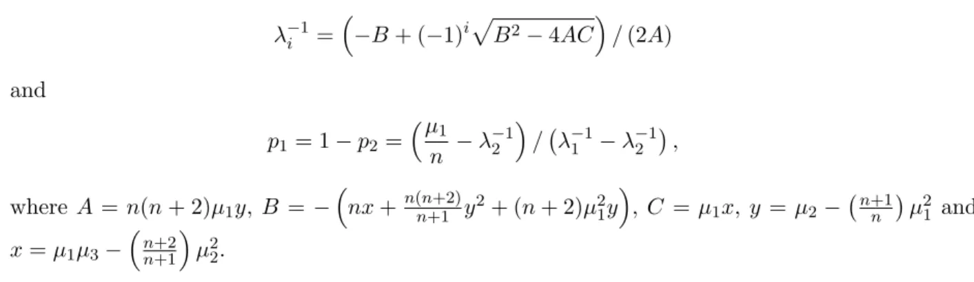
where µ(n)1 and µ(n)2 are the respective n-th moment of two Erlang distributions. Under some conditions, Theorem 3 of Johnson and Taaffe (1989) gives the parameters of the mixture of two Erlang distributions with the same order n as follows
λ−1i = ( −B + (−1)i√B2− 4AC)/ (2A) and p1 = 1− p2= (µ 1 n − λ −1 2 ) /(λ−11 − λ−12 ), where A = n(n + 2)µ1y, B = − ( nx +n(n+2)n+1 y2+ (n + 2)µ21y ) , C = µ1x, y = µ2− (n+1 n ) µ21 and x = µ1µ3− ( n+2 n+1 ) µ22.
For the numerical illustration, suppose that X ∼ Exp(λ = 1/100), the interclaim time distri-bution parameters β = 1, 5 and 10, the interest rate δ = 4%. We use three different values for the copula parameter θ =−1, 0, 1 and fix the time t = 5. The m-th moment of X is
E[Xm] = 1 λmm!.
As E[(X′m] =∫0∞mxm−1(1− FX(x))2dx, we have that
E[(X′m] = 1 (2λ)mm!.
The first three moments of Z(t) and the matched parameters for the mixture of Erlang distributions are presented in Tables1,2and 3.
θ µZ(5) µ (2) Z (5) µ (3) Z (5) n λ1 λ2 p1 p2 -1 477.682 3.346× 10⁵ 2.967× 10⁸ 3 0.0442 0.00563 0.119 0.881 0 453.173 2.878× 10⁵ 2.277× 10⁸ 4 0.0263 0.00747 0.215 0.785 1 428.664 2.434× 10⁵ 1.679× 10⁸ 4 0.0430 0.00867 0.088 0.911
Table 1: Moments of Z(5) and parameters of the mixture of Erlang distributions for β = 1. For this last case, Figures1,2and 3in the appendix show the drawings of the simulated c.d.f. of Z(5) versus the approximated c.d.f. of Z(5) with a mixture of Erlang distributions moment matching. We see on our illustration that the fit of the approximations is satisfying.
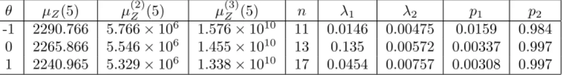
θ µZ(5) µ (2) Z (5) µ (3) Z (5) n λ1 λ2 p1 p2 -1 2290.766 5.766× 10⁶ 1.576× 10¹⁰ 11 0.0146 0.00475 0.0159 0.984 0 2265.866 5.546× 10⁶ 1.455× 10¹⁰ 13 0.135 0.00572 0.00337 0.997 1 2240.965 5.329× 10⁶ 1.338× 10¹⁰ 17 0.0454 0.00757 0.00308 0.997
Table 2: Moments of Z(5) and parameters of the mixture of Erlang distributions for β = 5.
θ µZ(5) µ (2) Z (5) µ (3) Z (5) n λ1 λ2 p1 p2 -1 4556.681 2.180× 10⁷ 1.091× 10¹¹ 21 0.0118 0.00459 0.00557 0.994 0 4531.731 2.136× 10⁷ 1.045× 10¹¹ 26 0.0118 0.00572 0.00605 0.994 1 4506.781 2.093× 10⁷ 9.999× 10¹⁰ 34 0.0157 0.00753 0.00326 0.998
Table 3: Moments of Z(5) and parameters of the mixture of Erlang distributions for β = 10. again, the approximated VaR’s are satisfying.
θ MC β = 1 MM β = 1 MC β = 5 MM β = 5 MC β = 10 MM β = 10 -1 1606.311 1620.153 4451.252 4498.420 7486.069 7545.406
0 1434.566 1426.921 4168.524 4220.984 7121.053 7166.169 1 1244.871 1251.674 3859.026 3895.557 6718.142 6755.696
Table 4: VaR calculated from the Monte-Carlo simulations and the moment matching.
Remark 1 Let S(t) = Z(t) when the force of interest δ = 0. As, in general for δ ≥ 0, we have E[φ(Z(t))] ≤ E[φ(S(t))] for every non-decreasing function φ, we have that Z(t) ≤sd S(t)
where ≤sd designate the stochastic dominance order. Furthermore, this implies that V aRα(Z(t))≤
V aRα(S(t)) for every α∈ [0, 1].
4.3 Solvency II internal model
The European Solvency II project is going to lay down some new regulatory requirements that every insurance company inside the European Union will have to fulfill. In addition, several other countries outside the European Union (e.g. Canada, Columbia or Mexico) are likely to use similar principles. The directive has been adopted in April 2009 and the implementation measures are in progress in order to have the new system in force on October 31st, 2012. Determination of Solvency Capital Requirement (SCR) is one of the main points of the quantitative pillar of this reform: in addition to the best estimate (which is defined as the expected present value of all potential future cash flows that would be incurred in meeting policyholders’ liabilities) of liabilities and a risk margin, insurance companies and reinsurers will have to own an extra capital to cope with unfavorable events. The computation of the Solvency II standard formula for SCR is based on the 1-year 99.5%-Value-at-risk (VaR). Most often in the standard formula, it is assumed that the heaviness of the tail of the distribution of random loss X is quite moderate, and so the SCR, defined as the difference V aR99.5%(X)− E(X), is replaced by a proxy qσX, where σX denotes the
standard error coefficient of X and q is a quantile factor which should be set at q = 3. Seldom, if appropriate, factor q = 3 may be replaced by a larger value, close to 5 for example, to take into account potential heavier tails. This is the case in particular in the current version of the Counterparty Risk module (see Consultation Paper 51 of CEIOPS). Although quantile factors may vary from one line of business to the other, it has become classical to compute the SCR in the standard formula as a multiple of the standard error coefficient of the random loss, or with stress scenarios. Even if internal models or partial internal models are being encouraged, companies will anyway have to provide the SCR computations with the standard formula as complement. Some of those partial internal models are based on a different time horizon, up to 5 or 10 years for some reinsurers. Besides, all insurers have to provide an Own Risk and Solvency Assessment (ORSA) which aims to study risks that may affect the long-term solvency of the company. Either for ORSA or for SCR computations, it may be useful to determine the first two moments of the discounted aggregate claim amount, both with constant interest rate and inflation, and in a stress scenario where inflation increases. Inflation is very low currently, but there is a clear risk that it increases quite a bit when the crisis ends. In an ORSA analysis, it would be interesting to study the impact of inflation on Best Estimate (BE) and on the SCR: what would be the BE and the SCR in three years from now if insurance risk exposure was the same as today, but inflation was much higher? This is what we investigate in Tables 6 and 7. Solvency II standard formula often uses the independence between claim amounts and the claim arrival process. In practice, for risks like earthquake risk or flood and drought risks, the next claim amount is not independent from the time elapsed before the previous claim, and this must be taken into account in partial internal models. The advantage of our method is that it remains valid for negative values of δ (as long as they are not too negative), which can be seen as the difference between the interest rate and the inflation rate. If inflation becomes larger than the interest rate, then δ becomes negative, and our method still applies for small enough values of |δ|. Some other approaches are possible as cat risk is sometimes addressed directly by the means of extreme scenarios.
Here we compute the SCR in the standard formula approach and in the internal model approach for a 5-year horizon for exponentially distributed inter-claim times and Exponential and Pareto claim amount distributions. For the internal model approach, we use Equations (??) and (??) from the previous example to compute the mth moment of Z(t) when the claim amounts are exponentially distributed. If the claim amount r.v. X is Pareto with c.d.f.
FX(x) = 1− ( γ γ + x )κ , x > 0, and mth moment E[Xm] = γ mm! ∏m i=1(κ− i) (21) for γ > 0 and κ > m then E[(X′m] becomes
E[(X′m] = γ
mm!
∏m
i=1(2κ− i)
. (22)
Thus the mth moment of Z(t) can be explicitly expressed using (10) and (16) for the first and second moments, or using (20) for greater moments. The SCR for the internal model is obtained
from the first moment of Z(t) and a simulated VaR with Monte-Carlo method.
Let the FGM dependence parameter be−1, 0 or 1, and δ = 3%. The parameter for the inter-claim time distribution is β = 2. Assume that the inter-claim amount r.v. X ∼ Exp(λ = 1/10) for the Exponential case and that X ∼ P areto(κ = 2.5, γ = 15) for the Pareto case with the same expected value 10 but with variances respectively equal to 100 and 500. As discussed above, we set the quatile factor q for the standard formula approach at 3 for the Exponential case and at 5 for the Pareto case. The SCR’s for the standard formula and the internal model approaches are presented in Table5. Using the internal model approach, we also compute the SCR (and the Best Estimate (BE)) with inflation crises (δ = 1.5%, 0.5% or −5%) in comparison to δ = 3% for the Pareto case. The results are shown in Table 6.
Exponential case Pareto case
Copula parameter Standard formula (q = 3) Internal model Standard formula (q = 5) Internal model
θ =−1 140.508 151.075 385.760 314.362
θ = 0 124.703 132.149 359.987 295.574
θ = 1 107.091 111.254 332.933 276.368
Table 5: Comparison between the standard formula and the internal model approaches for the SCR, 5-year time horizon.
Copula parameter δ = 3% δ = 1.5% δ = 0.5% δ =−5% θ =−1 BE 95.963 99.455 101.881 116.775 SCR 314.362 325.107 331.891 383.146 θ = 0 BE 92.861 96.342 98.760 113.610 SCR 295.574 306.034 313.842 362.76O θ = 1 BE 89.760 93.229 95.639 110.446 SCR 276.368 287.600 295.391 342.066
Table 6: Effect of inflation crisis for Pareto claim amounts, 5-year time horizon.
We also provide some results for the same values for δ when the time horizon is equal to 10 years and the copula parameter θ = 1 in Table 7.
Finally, we also provide in Table8 a few results with θ = 1 and β = 0.5 to see the influence of parameter β and to illustrate the case where large claims occur in average every m years, with m > 1.
Regarding dependency between inter-claim times and claim amounts, both SCR and Best Estimate are increasing with the dependence parameter θ. This is logical as positive dependence between inter-claim times and claim amounts is a form of diversification effect. SCR are larger for Pareto claim amounts than for Exponential claim amounts, as usual. Nevertheless, Table 5 shows that the so-called internal model approach leads to higher values of SCR than the ones obtained by the
δ = 3% δ = 1.5% δ = 0.5% δ =−5% θ = 1
BE 169.686 182.609 191.961 256.324 SCR 356.386 383.095 402.398 543.695
Table 7: Effect of inflation crisis for Pareto claim amounts, 10-year time horizon. δ = 3% δ = 1.5% δ = 0.5% δ =−5%
θ = 1
BE 40.163 43.352 45.661 61.583 SCR 182.448 197.233 207.688 284.735
Table 8: Effect of inflation crisis for Pareto claim amounts, 10-year time horizon, β = 0.5. standard formula for Exponentially distributed claim amounts, while it is the opposite for Pareto distributed claim amounts. Finally, the impact of inflation cannot be neglected: in Table 8, the case where δ = −5% (which corresponds to scenarios where the inflation rate becomes 5% larger than the interest rate) leads to more than a 50%-increase in Best Estimate and SCR, in the most favorable case where θ = 1.
5
Acknowledgements
The research was financially supported by the Natural Sciences and Engineering Research Council of Canada, the Chaire d’actuariat de l’Universit´e Laval, and the ANR project ANR-08-BLAN-0314-01. H. Cossette and E. Marceau would like to thank Prof. Jean-Claude Augros and the members of the ISFA for their hospitality during the stays in which this paper was made.
References
Albrecher, H. and Boxma, O. J. (2004). A ruin model with dependence between claim sizes and claim intervals. Insurance Math. Econom., 35(2):245–254.
Albrecher, H. and Teugels, J. L. (2006). Exponential behavior in the presence of dependence in risk theory. J. Appl. Probab., 43(1):257–273.
Asimit, A. and Badescu, A. (2009). Extremes on the discounted aggre-gate claims in a time dependent risk model. Scand. Actuar. J. from http://www.informaworld.com/10.1080/03461230802700897.
Baeumer, B. (2003). On the inversion of the convolution and Laplace transform. Trans. Amer. Math. Soc., 355(3):1201–1212 (electronic).
Biard, R., Lef`evre, C., Loisel, S., and Nagaraja, H. (2009). Asymptotic finite-time ruin probabilities for a class of path-dependent claim amounts using Poisson spacings. Talk at 2b) or not 2b) Conference, Lausanne, Switzerland.
Boudreault, M., Cossette, H., Landriault, D., and Marceau, E. (2006). On a risk model with dependence between interclaim arrivals and claim sizes. Scand. Actuar. J., (5):265–285.
Cossette, H., Marceau, ´E., and Marri, F. (2009). Analysis of ruin measures for the classical com-pound poisson risk model with dependence. To appear in Scandinavian Actuarial Journal. In press.
Delbaen, F. and Haezendonck, J. (1987). Classical risk theory in an economic environment. Insur-ance Math. Econom., 6(2):85–116.
Duchesne, T. and Marri, F. (2009). General distributional properties of discounted warranty costs with risk adjustment under minimal repair. IEEE Transactions on Reliability, 58(1):143–151. Jang, J. (2004). Martingale approach for moments of discounted aggregate claims. Journal of Risk
and Insurance, pages 201–211.
Jang, J. (2007). Jump diffusion processes and their applications in insurance and finance. Insurance Math. Econom., 41(1):62–70.
Johnson, M. A. and Taaffe, M. R. (1989). Matching moments to phase distributions: Mixtures of erlang distributions of common order. Stoch. Models, 5(4):711–743.
Kalashnikov, V. and Konstantinides, D. (2000). Ruin under interest force and subexponential claims: a simple treatment. Insurance Math. Econom., 27(1):145–149.
Kim, B. and Kim, H.-S. (2007). Moments of claims in a Markovian environment. Insurance Math. Econom., 40(3):485–497.
L´eveill´e, G. and Garrido, J. (2001a). Moments of compound renewal sums with discounted claims. Insurance Math. Econom., 28(2):217–231.
L´eveill´e, G. and Garrido, J. (2001b). Recursive moments of compound renewal sums with discounted claims. Scand. Actuar. J., (2):98–110.
L´eveill´e, G., Garrido, J., and Wang, Y. (2009). Moment generating functions of compound renewal sums with discounted claims. To appear in Scandinavian Actuarial Journal.
Nelsen, R. B. (2006). An introduction to copulas. Springer Series in Statistics. Springer, New York, second edition.
Porter, K., Beck, J., Shaikhutdinov, R., Au, S., Mizukoshi, K., Miyamura, M., Ishida, H., Moroi, T., Tsukada, Y., and Masuda, M. (2004). Effect of seismic risk on lifetime property value. Earthquake Spectra, 20(4):1211–1237.
Ren, J. (2008). On the Laplace Transform of the Aggregate Discounted Claims with Markovian Arrivals. N. Am. Actuar. J., 12(2):198.
Rolski, T., Schmidli, H., Schmidt, V., and Teugels, J. (1999). Stochastic processes for insurance and finance. Wiley Series in Probability and Statistics. John Wiley & Sons Ltd., Chichester. Sundt, B. and Teugels, J. L. (1995). Ruin estimates under interest force. Insurance Math. Econom.,
16(1):7–22.
Tang, Q. (2005). The finite-time ruin probability of the compound Poisson model with constant interest force. J. Appl. Probab., 42(3):608–619.
Taylor, G. C. (1979). Probability of ruin under inflationary conditions or under experience rating. Astin Bull., 10(2):149–162.
Tijms, H. (1994). Stochastic models: an algorithmic approach. John Wiley, Chiester.
van Noortwijk, J. and Frangopol, D. (2004). Two probabilistic life-cycle maintenance models for deteriorating civil infrastructures. Probabilistic Engineering Mechanics, 19(4):345–359.
Waters, H. (1983). Probability of ruin for a risk process with claims cost inflation. Scand. Actuar. J., pages 148–164.
Willmot, G. E. (1989). The total claims distribution under inflationary conditions. Scand. Actuar. J., (1):1–12.
Yang, H. and Zhang, L. (2001). On the distribution of surplus immediately after ruin under interest force. Insurance Math. Econom., 29(2):247–255.
APPENDIX
The first two moments of the distribution of Z(t) which are given by (10) and (16) respectively. The third moment is
µ(3)(t) = 3 ∑
n=1
∑
((i1,j1,k1),...,(in,jn,kn))∈A3n
I (ζ(i1; j1; k1); ...; ζ(in; jn; kn)) , where A3n = { (i1, j1, k1), ..., (in, jn, kn); i1 = 3, i1+ ... + in= 3− 1 + n, i1 > ... > in, j1 = 3 + 1− n, j1+ ... + jn= 3, j1≥ ... ≥ jn, k.∈ {0, 1} } . It can be developed as µ3(t) = (3 3 ) βE[X3] ( 1 3δ− e−3δt 3δ ) + (3 3 ) θβ(E[X′3]− E[X3 ]) ( 1 2β + 3δ− e−(2β+3δ)t 2β + 3δ ) + (3 2 )(1 1 ) β2E[X]E[X2] ( 1 3δ2− e−δt 2δ2 + e−3δt 6δ2 ) + (3 2 )(1 1 )
θβ2E[X2](E[X′]− E[X]) ( 1
3δ (2β + δ)− e−(2β+δ)t (2β + δ) (−2β + 2δ)+ e−3δt 3δ (−2β + 2δ) ) + (3 2 )(1 1 )
θβ2E[X](E[X′2]− E[X2]) ( 1 δ (2β + 3δ)− e−δt δ (2β + 2δ)+ e−(2β+3δ)t (2β + 3δ) (2β + 2δ) ) + (3 2 )(1 1 )
θ2β2(E[X′]− E[X]) (E[X′2]− E[X2
]) ( 1 (2β + δ) (2β + 3δ)− e−(2β+δ)t 2δ (2β + δ)+ e−(2β+3δ)t 2δ (2β + 3δ) ) + (3 1 )(2 2 ) β2E[X]E[X2] ( 1 6δ2− e−2δt 2δ2 + e−3δt 3δ2 ) + (3 1 )(2 2 )
θβ2E[X](E[X′2]− E[X2]) ( 1
3δ (2β + 2δ)− e−(2β+2δ)t (2β + 2δ) (−2β + δ)+ e−3δt 3δ (−2β + δ) ) + (3 1 )(2 2 )
θβ2E[X2](E[X′]− E[X]) ( 1
2δ (2β + 3δ)− e−2δt 2δ (2β + δ)+ e−(2β+3δ)t (2β + δ) (2β + 3δ) ) + (3 1 )(2 2 )
θ2β2(E[X′]− E[X]) (E[X′2]− E[X2]) ( 1
(3β + 2δ) (2β + 3δ)− e−(2β+2δ)t δ (2β + 2δ) + e−(2β+3δ)t δ (2β + 3δ) ) + (3 1 )(2 1 )(1 1 ) β3E[X]3 ( 1 6δ3− e−δt 2δ3 + e−2δt 2δ3 − e−3δt 6δ3 ) + (3 1 )(2 1 )(1 1 )
θβ3E[X]2(E[X′]− E[X]) ( 1
3δ2(2β + δ)− e−(2β+δ)t (2β + δ) (−2β + δ) (−2β + 2δ)+ e−2δt 2δ2(−2β + δ)− e−3δt 3δ2(−2β + 2δ) ) + (3 1 )(2 1 )(1 1 )
θβ3E[X]2(E[X′]− E[X]) ( 1
3δ2(2β + 2δ)− e−δt 2δ2(2β + δ)+ e−(2β+2δ)t (2β + 2δ) (2β + δ) (−2β + δ)− e−3δt 6δ2(−2β + δ) ) + (3 1 )(2 1 )(1 1 )
θβ3E[X]2(E[X′]− E[X]) ( 1 2δ2(2β + 3δ)− e−δt δ2(2β + 2δ)+ e−2δt 2δ2(2β + δ)− e−(2β+3δ)t (2β + 3δ) (2β + 2δ) (2β + δ) ) + (3 1 )(2 1 )(1 1 ) θ2β3E[X] ( E[X′]− E[X] )2( 1 3δ (2β + δ) (2β + 2δ)− e−(2β+δ)t δ (2β + δ) (−2β + 2δ)+ e−(2β+2δ)t δ (2β + 2δ) (−2β + δ)− e−3δt 3δ (−2β + 2δ) (−2β + δ) ) + (3 1 )(2 1 )(1 1 )
θ2β3E[X](E[X′]− E[X])2
( 1 2δ (2β + δ) (2β + 3δ)− e−(2β+δ)t 2δ (2β + δ) (−2β + δ)+ e−2δt 2δ (−2β + δ) (2β + δ)− e−(2β+3δ)t 2δ (2β + 3δ) (2β + δ) ) + (3 1 )(2 1 )(1 1 )
θ2β3E[X](E[X′]− E[X])2
( 1 δ (2β + 2δ) (2β + 3δ)− e−δt δ (2β + δ) (2β + 2δ)+ e−(2β+2δ)t δ (2β + 2δ) (2β + δ)− e−(2β+3δ)t δ (2β + 3δ) (2β + 2δ) ) + (3 1 )(2 1 )(1 1 ) θ3β3(E[X′]− E[X])3 ( 1 (2β + δ) (2β + 2δ) (2β + 3δ)− e−(2β+δ)t 2δ2(2β + δ)+ e−(2β+2δ)t δ2(2β + 2δ)− e−(2β+3δ)t 2δ2(2β + 3δ) )
Figure 1: