HAL Id: halshs-00974144
https://halshs.archives-ouvertes.fr/halshs-00974144
Submitted on 5 Apr 2014
HAL is a multi-disciplinary open access
archive for the deposit and dissemination of sci-entific research documents, whether they are pub-lished or not. The documents may come from
L’archive ouverte pluridisciplinaire HAL, est destinée au dépôt et à la diffusion de documents scientifiques de niveau recherche, publiés ou non, émanant des établissements d’enseignement et de
Optimism, pessimism and financial bubbles
Bertrand Wigniolle
To cite this version:
Bertrand Wigniolle. Optimism, pessimism and financial bubbles. Journal of Economic Dynamics and Control, Elsevier, 2014, 41, pp.188-208. �10.1016/j.jedc.2014.01.022�. �halshs-00974144�
Optimism, pessimism and …nancial bubbles
B. Wigniolle
yJanuary 17, 2014
Abstract
This paper shows that it is possible to extend the scope of the existence of rational bubbles when uncertainty is introduced associ-ated with rank-dependent expected utility. This RDU assumption can be viewed as a transformation of probabilities depending on the pessimism/optimism of the agent. The results show that pessimism favors the existence of deterministic bubbles, when optimism may pro-mote the existence of stochastic bubbles. Moreover, under pessimism, the RDU assumption may generate multiple bubbly equilibria. The RDU assumption also leads to new conditions ensuring the (absence of) Pareto-optimality of the competitive equilibrium without bubbles. These conditions still govern the existence of bubbles. JEL classi…ca-tion: D81, D9, G1, O41. Keywords: rational bubbles, RDU prefer-ences.
I thank an editor of JEDC and three anonymous referees for helpful comments. I am grateful to Michèle Cohen, Mégléna Jéléva and Jean-Christophe Vergnaud for stimulating discussions on the RDU model. I thank the participants at the conference "New challenges for macroeconomic regulation: …nancial crisis, stabilisation policy and sustainable develop-ment", Marseille 2011, for their helpful comments, and particularly Lise Clain-Chamosset, Thomas Seegmuller and Robert Becker. This paper was also presented at the 11th SAET Conference. I thank Jean-Marc Bonnisseau for his invitation and the participants at his session for their comments.
yParis School of Economics, University of Paris 1 Pantheon-Sorbonne. Address: C.E.S.,
106-112, boulevard de l’hôpital, 75647 Paris Cedex 13, France. Tel: +33 (0)1 44 07 81 98. Email : [email protected].
1
Introduction
This paper shows that the scope for the existence of rational bubbles can be extended when uncertainty and rank-dependent expected utility are intro-duced. In the framework of an overlapping generations model à la Diamond (1965), the seminal article by Tirole (1985) proves that bubbles can arise in economies for which the return on capital at a steady state is below the growth rate of output. The bubbleless economy must be in a state of overac-cumulation that corresponds to dynamic ine¢ciency. Weil (1987) proposes a model of stochastic bubbles using the same framework as Tirole, and …nds existence conditions that are even stronger. Di¤erent authors have intro-duced rational bubbles in richer frameworks with endogenous growth (e. g. Grossman and Yanagawa, 1993 and Olivier, 2000). But the existence of bub-bles remains linked to the same condition between the growth rate and the interest rate. As empirical observations suggest that this condition is not ful…lled in general (see Abel et al. 1989), rational bubbles seem unlikely to arise. They may perhaps not be the pertinent explanation to understand bubble phenomena that actually are observed.
In recent contributions, Caballero and Hammour (2002) and Caballero et al. (2006) obtain the existence of bubbles under less stringent conditions at the price of a transformation of the notion of bubble. They build an overlapping generations model with an adjustment cost to capital leading to two long-run equilibria. They interpret the equilibrium corresponding to a higher valuation of the capital stock as a bubbly1 equilibrium.
This paper intends to show that it is possible to extend the scope for the existence of rational bubbles when uncertainty is introduced associated with a rank-dependent expected utility. A simple overlapping generations model is studied in which the production technology depends on a technological shock: capital return is random. In order to have a very tractable model, there are only two possible states of the nature and the capital return may oscillate between a high and a low value. In an economy in which capital is the only asset, …nancial markets are incomplete as two states of the nature
1This paper uses the terminology introduced by Tirole (1985) and employs the
exist. The existence of a bubbly asset can make …nancial markets complete. Two types of bubbles are considered in this context. The …rst type, called a deterministic bubble, is an asset that has the same price in both states of the nature. The second type, called a stochastic bubble, is an asset whose existence is conditional to the occurrence of a particular state of the nature. As in Weil (1987), agents form their expectations according to a self-ful…lling prophecy which assumes that the bubble will burst if the other state arises.
Moreover, it is assumed that agents are endowed with a rank-dependent expected utility (RDU) function. This model has been introduced by Quig-gin (1993) and developed by Chateauneuf (1999). A general presentation can be found in Cohen and Tallon (2000). The RDU model can be viewed as a generalization of the standard EU (Expected Utility) model, based on the Von Neumann Morgenstern’s axioms. In a famous paper, Allais (1953) has showed through experiments that a majority of people do not behave accord-ing to the expected utility model, as their actions violate the independence axiom. The RDU model is based on a weaker form of this independence axiom that can reconcile the theory with some actual behaviors.
According to the RDU model, the distribution of probabilities is trans-formed by a probability weighting function (pwf). The utility is no longer linear with respect to the probabilities of the states of nature. This assump-tion can be viewed as a transformaassump-tion of probabilities depending on the pessimism/optimism of the agent. A pessimistic agent will give more weight to the bad state of the nature, whereas an optimistic agent will give more weight to the good state. This assumption has two implications. Firstly, the deformation of probabilities may lead to quantitative changes with respect to the ones obtained with the standard EU (Expected Utility) model. More precisely, our results show that pessimism favors the existence of determin-istic bubbles and of small stochastic bubbles, while optimism may promote the existence of big stochastic bubbles. Secondly, the deformation of prob-abilities depends on the rank of the consumptions in the di¤erent states of the nature. It will be shown that this property may lead to a multiplicity of bubbly equilibria.
Considering pessimistic agents in the case of a deterministic bubble, the transformation of probabilities weakens the existence conditions of a
bub-ble. The interpretation is simple. By assumption, the gross capital return is greater than 1 in the good state of the nature, while it is smaller than 1 in the bad state. Investing in the bubble provides a gross return equal to 1. Agents invest in the bubble in order to be protected against the occurrence of the bad state. In the case of pessimism, they put more weight on this state and invest more in the bubble. Therefore, pessimism may support the bubble.
In the case of a stochastic bubble, it is assumed that the existence of the bubble is conditional to the state with a low capital return, the bubble bursting in the state with a high capital return.2 This assumption may
reverse the rank of the states of the nature. With a deterministic bubble, as this asset provides the same gain in the two states of the nature, the state with a high capital return is always the best state of the nature. With a stochastic bubble, the state with a low capital return also corresponds to the continuation of the bubble. Therefore, if the bubble has a high value, it is possible that the state with a low capital return becomes the best state of the nature. But if the bubble has a low value, the state with a high capital return remains the best state of the nature. As the transformation of probabilities in the RDU model depends on the rank, two types of bubbly equilibria may exist, associated with a low value or a high value of the bubbly asset.
Optimism promotes the existence of an equilibrium with a high value of the bubble. As the good state for the consumer corresponds to the existence of the bubble, optimistic agents assign more weight to the bubbly state and invest more in the bubble. In the end, optimism favors stochastic bubbles. In contrast, pessimism plays in favor of the existence of an equilibrium with a low value of the bubble. In this case, the bubbly state is the bad state of nature for the consumer. A pessimistic agent assigns more weight to this state, which favors the existence of a bubbly equilibrium.
The case of a stochastic bubble is particularly interesting under the RDU assumption, as it leads to two types of bubbly equilibria associated with either a low price or a high price for the bubble. Increasing the degree of pessimism can have both a positive or a negative e¤ect on the existence of a bubbly equilibrium. Pessimism promotes the existence of a bubble with a low
price, whereas optimism plays in favor of a bubble with a high price. These results come from the property that the weights put on the di¤erent states of the nature depend on the rank within the RDU framework. A stochastic bubble with a low value does not change the ranking of the two states of the nature whereas a bubble with a high value does. Therefore, the same parameter - the degree of optimism - can have opposite e¤ects depending on the type of bubbly equilibrium.
Finally, in the case of pessimism and stochastic bubbles, an equilibrium may exist associated with a value of the bubble such that the two states of nature lead to equal levels of consumption. Moreover, this bubbly steady state may be stable and there is convergence with oscillations. There exists an in…nity of initial conditions for the value of the bubble and the bubbly equilibrium is indeterminate. The existence of such an equilibrium is due to the "kink" in the indi¤erence curves which appears for equal levels of consumption, in the two states of nature in the RDU framework.
This result can be related to previous ones obtained in …nance literature with rank dependent utility or Choquet utility: Tallon (1997) and Epstein and Wang (1994) also obtain the existence of multiple equilibria. The orig-inality of this work is to obtain the result in a production economy with capital and a bubbly asset. In an exchange economy, the dynamics of as-set prices is completely governed by the history of exogenous shocks. In a production economy with capital, the dynamics of asset prices also depend on the dynamics of capital accumulation. As simple parametric forms are used in the model, the dynamics of the bubbly asset can be explicitly de-termined: the price converges with oscillations toward its long run value. Bosi and Seegmuller (2010) have also developed a framework in which there exists an indeterminate bubbly equilibrium. In their model, indeterminacy is due to frictions introduced via a cash-in-advance constraint with …nancial market imperfections. In this work, indeterminacy is obtained in a model in which the only …nancial market imperfection comes from incomplete markets associated with RDU preferences.
This paper successively considers di¤erent assumptions: EU preferences, RDU preferences, deterministic bubbles, and stochastic bubbles. For each case, the existence conditions of bubbles are related to the Pareto optimality
properties of the economy without bubbles. The study of Pareto optimality is based particularly on previous articles that have studied Pareto optimality of allocations in overlapping generations models with stochastic shocks, such as Peled (1984), Peled and Aiyagari (1991), Wang (1993), Gottardi (1996) and Demange and Laroque (1999).
As expected, bubbles can only appear in an economy for which the com-petitive equilibrium is not Pareto optimal. For RDU preferences, the condi-tion ensuring Pareto optimality also depends on the transformacondi-tion of prob-abilities implied by the pessimism/optimism of the agents. Therefore, it cannot be reduced to a comparison between the interest rate and the growth rate of the economy. It provides an additional degree of freedom that may reconcile the existence of bubbles with parameters that are empirically rel-evant. The link between dynamic e¢ciency and the existence of bubbles has been questioned recently in contributions that introduce capital market imperfections: in Farhi and Tirole (2012), …rms are …nancially constrained and demand and supply liquidity; in Martin and Ventura (2012), investors can be "productive" or "unproductive" and productive investors cannot bor-row from unproductive ones. In these two contributions, the assumption of imperfect capital markets tends to disentangle the existence of bubbles from dynamic ine¢ciency.
Our approach can be related to a recent literature in behavioral economics that explains bubbles and …nancial anomalies by deviations from rationality. Irrationality can be related both to behaviors and to expectations. A general presentation can be found in Hommes (2006). In these models, anomalies in …nancial markets may result from the bounded rationality of agents associ-ated with their heterogeneity. Agents behave according to di¤erent heuristic rules and make various expectations. In such a framework, Boswijk et al. (2007) shows that two expectation regimes may exist: a "fundamentalists regime" in which agents believe in the reversion of stock prices toward the fundamental value, and a "chartist, trend following regime" in which agents expect persisting deviations from the fundamental value. When behavioral heterogeneity exists, more hedging instruments may destabilize markets, as it is shown in Brock et al. (2009). Some experimental results may support
the behavioral assumption, as Hommes et al. (2008). This article presents a controlled experiment in which subjects must expect the price of a risky asset, a computer calculating the optimal trading decisions resulting from rational behaviors and the equilibrium price. In the experiment, prices may deviate from their fundamental value and bubbles may emerge, that seem inconsistent with rational expectations. With respect to this literature, our approach may be viewed as developing the foundation of behaviors, using the new theories of decision under uncertainty. As discussed in Machina (1989), the RDU assumption introduces some deviation with respect to the "full" rationality implied by the EU assumption. It is a way to give a pre-cise sense to the notions of optimism and pessimism. A generalization of our model could be to incorporate heterogeneous agents in their degree of optimism/pessimism, in order to have di¤erent speculative behaviors. The assumption of rational expectations could also be relaxed, either by an ad-hoc expectation rules, or by the assumption of a reduced information set for the agents.
Our work can also give foundations to a long tradition in economics which emphasizes the role of optimism in the development of …nancial bubbles. In the famous book "Manias, panics and crashes: a history of …nancial crises", Kindleberger and Aliber argue that investors become more optimistic in ex-pansion phases, which contributes to the development of bubbles. This view also corresponds to Minsky’s model developed in 1982 that stresses the …-nancial instability hypothesis. These theories have enjoyed some popularity in the media and it is often referred to waves of optimism or exuberance to explain bubbles phenomenon. As discussed above, the RDU assumption allows to give a precise sense to the notions of optimism and pessimism. In a general equilibrium model, the e¤ect of optimism can be counterintuitive and can challenge the standard view: pessimism may play in favor of bubbles when the investors use the bubbly asset as a coverage strategy against risk.
Section 2 presents the basic framework with EU preferences and a com-petitive equilibrium without bubbles. A condition ensuring the Pareto op-timality of this equilibrium is derived. Section 3 studies the existence of deterministic and stochastic bubbles in this framework. Section 4 concludes. All proofs of propositions are presented in Section 5. A last Appendix
(Ap-pendix 7 in Section 6) is available as online material for a supplementary …le published online alongside the electronic version. It is also available upon request, or in Wigniolle (2012).
2
The basic model
The basic setup is an overlapping generations model with capital accumula-tion à la Allais (1947)-Samuelson (1958)-Diamond (1965). Agents live during two periods. They supply one unit of labor in the …rst period (when young) and they are retired and consume the proceeds of their savings in the second period (when old). The number of agents in each generation is normalized to 1. In this part, capital is the only asset that can be held by agents and there is no bubble.
2.1
Production
There is a single good in the economy, produced in period t with capital Kt 1
(the capital stock results from t 1 investment) and labor Lt. In each period
t exists one competitive …rm using a linear production technology
Yt = R( t)Kt 1+ wLt
Capital depreciation is completed in one period. Labor productivity is con-stant and equal to w: Capital productivity R( t) follows a random process
that depends on the state of the nature t: At each period t, t 2 f1; 2g :
State 1 occurs with probability and state 2 with probability 1 : For
t= i; i = 1; 2; R(i) will be denoted Ri and it is assumed that
R1 > 1 > R2 (1)
In each period t; t is known by agents before they make their choices.
Under perfect competition, it is straightforward that w will be the equilibrium value of the wage and R( t) the capital gross rate of return.
As in Demange and Laroque (1999), a linear production technology is used. This assumption can also be interpreted as an exchange economy framework, with w as the endowment of each young agent, and R( t) as the
exogenous stochastic return of a storage technology. It allows to have explicit results only depending on the structural parameters of the economy.
We can wonder on the robustness of the results to other speci…cations for the production technology. This question is studied in an Appendix 7 that is available online as supplementary content. This appendix considers the two types of equilibria that are studied in the paper - equilibrium with a non-exploding bubble, equilibrium with an non-exploding bubble - with more general assumptions on the production technology. For the …rst type of bubble, two results are shown. With a Cobb-Douglas production function, uncertainty does not a¤ect the existence of a long run bubbly equilibrium. Therefore, pessimism or optimism do not in‡uence the existence of bubbles. With a CES production function, for a high elasticity of substitution, the results that were obtained with a linear production technology are kept: bubbly equilibria may exist and are favored by pessimism.
For exploding bubbles, assuming a CES production function with an elas-ticity of substitution greater than 1; two results of the paper are kept: pes-simism favors the existence of small stochastic bubbles whereas optimism favors the existence of big stochastic bubbles.
These di¤erent results obtained with Cobb-Douglas or CES production technologies reveal the crucial role played by the elasticity of substitution in the existence of bubbly equilibria. In the case of non-exploding bubbles, the numerical simulations show that an increase in the elasticity of substitution gives the same type of result than an increase in pessimism. In the case of exploding bubbles, a formal condition can be derived that show that the elasticity of substitution must be higher than some threshold value in order to have bubbly equilibria.
The elasticity of substitution plays a role as it governs the relative impact for labor and capital incomes of a technology shock on the capital stock. In the Cobb-Douglas case, a technological shock on the capital stock a¤ects in the same way the productivity of labor. This is the well-known property that a Solow-neutral technical progress is also Hicks-neutral and Harrod-neutral. From Abel et al. (1989), it is known that dynamic ine¢ciency needs that gross investment exceeds capital income. For a Cobb-Douglas technology associated with homothetic preferences, capital income and gross investment
are a¤ected in the same way by a technology shock and uncertainty has no impact on the existence of bubbles.3 For a CES production technology
with an elasticity of substitution greater that 1, capital income and gross investment are not a¤ected in the same way by the technological shock. Therefore, the conditions ensuring dynamic ine¢ciency and the existence of bubbles depend on uncertainty. In the limit case of a linear technology (in…nite elasticity of substitution), labor income is not hit by the shock and uncertainty has the higher impact.
2.2
Budget constraints and preferences
An agent born in t knows the state of the economy for t; but not for t + 1: ct is the …rst period consumption, st is the amount of investment in physical
capital, and dt+1 is the second period consumption that is a random variable
in t. The budget constraints are:
ct+ st = w (2)
dt+1 = R( t+1)st (3)
The agent is endowed with an intertemporal utility function. By assumption, this function corresponds to a rank-dependent expected utility (RDU), which is a generalization of the standard expected utility model. In the expected utility framework, the preferences of a generation t are based on the function:
u(ct) + Et[u(dt+1)] (4)
with Etthe expectation taken in period t and u the Von Neumann and
Mor-genstern utility function (VNM). To have simple calculations, the particular case u(x) = ln(x) will be considered.
A more general assumption will be used through this paper, the assump-tion of a rank-dependent expected utility (RDU) funcassump-tion. This model was initiated by Quiggin (1993) and developed by Chateauneuf (1999). It can be viewed as a generalization of the standard EU (Expected Utility) model, based on the Von Neumann Morgenstern’s axiomatic. As it was shown by
Allais (1953) with his so-called Allais’ Parodox, a majority of people do not behave according to the independence axiom of the EU theory. The RDU model is based on a weaker form of this independence axiom that can recon-cile the theory with some actual behaviors.
Following Quiggin (1993), the distribution of probabilities is transformed by a probability weighting function (pwf) : is a continuous increasing function from [0; 1] to [0; 1] such that (0) = 0 and (1) = 1:
With this assumption, the preceding utility function (4) must be trans-formed according to the following rules.
Denoting c; d1 and d2; the consumption levels when young, when old in
the state 1 and old in the state 2; the utility function is:
if d1 > d2; ln c + ( ) ln(d1) + [1 ( )] ln(d2) (5) = ln c + ln(d2) + ( ) ln(d1) ln(d2) if d1 < d2; ln c + [1 (1 )] ln(d1) + (1 ) ln(d2) (6) = ln c + ln(d1) + (1 ) ln(d2) ln(d1)
In each case, the second formulation allows to have more intuition on the RDU assumption. If d1 > d2; the term ln(d2) represents the minimum
utility level that the agent will have without risk in the second period. With a probability ; she/he will enjoy an additional gain of [ln(d1) ln(d2)] : In
the calculation of the expected gain, this probability is transformed in ( ): If d1 < d2; the minimum utility level is now ln(d1): With a probability
1 that is transformed in (1 ); he/she will enjoy the additional gain of (1 ) [ln(d2) ln(d1)] : As a consequence of these assumptions, the
formulation of the utility function depends on the rank of the variables d1
and d2:
In abbreviated form, the utility function will be denoted by:
where E is the expected value calculated with the transformed probabilities according to (5) and (6), and d is the random variable (d1; d2; ; 1 ) :
The property ( ) < can be interpreted as pessimism and ( ) > as optimism. An optimistic agent puts more weight on the best state of the nature, whereas a pessimistic agent puts more weight on the worst state.
The following notations will be used from now: 1 = ( ) and 2 =
1 (1 ). Therefore, for a pessimistic agent, 1 < < 2; and for an
optimistic agent 1 > > 2: For ( ) = ; the EU model is recovered and 1 = = 2. The function gives to the RDU model an additional degree
of freedom.
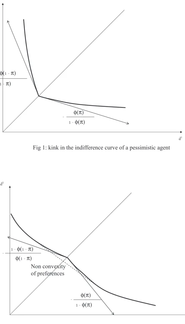
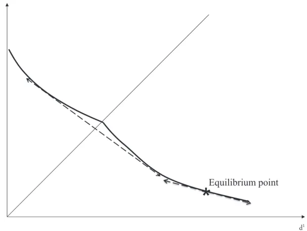
The RDU assumption has two main consequences. The …rst one corre-sponds to the deformation of probabilities, that may lead to quantitative changes: with respect to the EU model, the agents behave as if they did not take into account the true probabilities. The second consequence corresponds to the existence of a kink in the indi¤erence curves for d1 = d2: Figures 1
and 2 represent an indi¤erence curve in the plane (d1; d2); for a given value
of c; in the case of a pessimistic or optimistic agent. When the curve crosses the line d1 = d2; the slope in absolute value is [1 (1 )] = (1 ) at
left and ( )= [1 ( )] at right. This feature comes from the formulation of the utility function that depends on the rank of the variables. In the pessimistic case, for d1 = d2; di¤erent values of prices may be admissible.
This property may imply qualitative changes in the results: in the literature on RDU preferences, it often generates multiple equilibria. In the optimistic case, preferences are no more convex, as for a given point (c; d1; d2) ; the set
f(c0; d10; d20) such that (c0; d10; d20) < (c; d1; d2)g is not convex (see Figure 2).
2.3
The competitive equilibrium without bubbles
From condition (1), it is clear that state 1 is the good state of the nature and state 2 the bad state in the economy without bubbles. Therefore, the utility function is always given by (5). Maximizing (5) under budget constraints (2)and (3) gives the results: ct = w 1 + st = w 1 + dt+1 = R( t+1) w 1 +
Results do not depend on ( ) as the utility function is log-linear. In this simple case, the RDU assumption gives the same results as the EU model.
The capital stock used in period t + 1 results from the investment in physical capitals in t :
Kt=
w 1 +
Therefore, after one period, the capital stock reaches a constant value. In t = 0; the initial value of the capital stock K 1 is given, as the
con-sumption level of the …rst old agent: d0 = R( 0)K 1:
2.4
Pareto optimality of the competitive path
2.4.1 De…nitionA standard result in OLG deterministic models (Tirole, 1985) is that the ex-istence of …nancial bubbles is possible only in economies that are dynamically ine¢cient. If uncertainty is removed from the model (R(1) = R(2) = R), dynamic e¢ciency is obtained for R > 1:
By dynamic e¢ciency, Tirole’s article refers to the criterion introduced by Cass (1972). This criterion is concerned with the e¢ciency of aggregate consumption in a deterministic model of growth. A more accurate concept for overlapping generations models has been developed by Homburg (1992) and De la Croix and Michel (2002). It takes into account the utility levels of the agents of the di¤erent generations and it corresponds to Pareto optimality.
In stochastic overlapping generations models, Zilcha (1991) derived a cri-terion of dynamic e¢ciency based on aggregate consumption that generalizes Cass’s criterion. But the appropriate concept for Pareto optimality in such frameworks is interim optimality, as it refers to the expected utility of the
agents and not only on aggregate consumption. It has been developed and used by Peled (1984) and Demange and Laroque (1999). It is the natural ex-tension of the standard notion of Pareto optimality to a dynamic framework with uncertainty. The formal de…nition of this concept is given in the proof of Proposition 1 (in Appendix 1). In order to keep the exposition simple, only a non formal de…nition is given in the text.
Interim optimality is de…ned on feasible allocations. In period t, the resource constraint of the economy can be expressed as:
ct+ dt+ Kt= R( t)Kt 1+ w (8)
A feasible allocation is an allocation (ct; dt; Kt)t 0; starting from a given value
for K 1; that satis…es the resource constraint (8) for all t: Note that ct; dt
and Kt are random variables that may take di¤erent values according to the
all history of technological shocks.
A feasible allocation is interim optimal if there does not exist another feasible path that gives higher expected utility (calculated with transformed probabilities) for all period t and all histories, with a strict improvement for at least one period and one state of the nature.
2.4.2 The expected utility framework
The Pareto optimality of the equilibrium is …rst studied under the EU as-sumption, with the utility function (4).
Proposition 1 If
R1
+1 R2
< 1 (9)
the competitive equilibrium is interim Pareto optimal.
Proof. See Appendix 1.
The proposition shows that interim Pareto optimality is preserved if the low value of R2 in the bad state is compensated by a high enough value
of R1 in the good state. It is interesting to note that if (9) holds, then
R1+ (1 )R2 > 1: Therefore, Pareto optimality needs a stronger condition
contributions in di¤erent frameworks have also pointed out this property (see e. g. Blanchard and Weil (2001) for instance). (9) can be written under the form:
> R1(1 R2) R1 R2
(10) A high probability for the good state plays in favor of the Pareto optimality of the equilibrium.
2.4.3 The RDU framework
What can be said about the Pareto optimality of the equilibrium with RDU preferences? It is necessary to study separately the cases of pessimistic and optimistic agents. In both cases, the utility function is not di¤erentiable at a point such that d1 = d2: But, if agents are pessimistic, their preferences
remain convex, whereas this property is lost for optimistic agents. In the …rst case, it is easy to adapt the result of Proposition 1.
Proposition 2 If agents are pessimistic and
1
R1
+1 1 R2
< 1 (11)
the competitive equilibrium without bubbles is interim Pareto optimal.
Proof. See Appendix 2.
This condition is the same as the one of Proposition 1, except that is replaced by 1: This is due to the transformation of probabilities in the
utility function of the agent. Considering the inequality under the form (10), as 1 < for a pessimistic agent, it is clear that pessimism is not favorable
to the Pareto optimality of the competitive equilibrium.
When agents are optimistic, as agents’ preferences are no longer convex, the preceding e¢ciency condition (11) is necessary but not su¢cient. An-other condition is needed that can be interpreted as a "moderate" optimism, or a weak transformation of the probabilities.
Proposition 3 Assuming optimistic agents, if
1
R1
+1 1 R2
and R2 R1 < " 2 1 (1 1)(1 2) 2 2 (1 2)(1 2) # 1 1 2 (13)
the competitive equilibrium without bubbles is interim Pareto optimal.
Proof. See Appendix 3.
Condition (13) guarantees that no other feasible allocation dominating the competitive equilibrium exists in the zone in which d1 < d2: More
pre-cisely, it is possible to represent in the plane (d1; d2) the point of the
indif-ference curve corresponding to the equilibrium. When (13) holds, this point is out of the zone delimited by the tangent line to the indi¤erence curve (see Figure 3).
A better intuition can be achieved in particular cases. The following corol-lary studies the limit condition obtained from (13) when the transformation of probabilities vanishes. Then, it takes a particular assumption for
( ) = ; with 0 < < 1
The lower ; the more optimistic the agent is.
Corollary 1 1. In the limit case 1 ! and 2 ! ; Condition (13)
becomes R2=R1 < 1, which is true by assumption. By continuity, (13)
is ful…lled if the transformation of probabilities is moderate.
2. Let us assume that ( ) = with 2 (0; 1): There exists a value 2 (0; 1) such that (13) is satis…ed if and only if > :
Proof. See Appendix 4.
The …rst part of the corollary shows that Condition (13) is satis…ed in the limit case 1 ! and 2 ! : By continuity, it is satis…ed if the
transformation of probabilities is not too strong. The second part introduces a particular function that allows the transformation of probabilities to be measured by the parameter : can be interpreted as the degree of pessimism (or as the opposite of the degree of optimism). The corollary allows a lower bound on to be de…ned that represents a limit value for the degree of optimism.
3
The equilibrium with …nancial bubbles
This section assumes the existence of a bubble asset. Following Tirole (1985) and Weil (1987), this asset is a pure bubble, with a fundamental value equal to 0: It plays the role of store of value but yields no transactions services. It is called "pieces of paper" by Tirole or "money" by Weil, and can be any good that cannot be consumed or used.
Two types of bubbles are studied: one is called a bubble "à la Tirole" which is "deterministic", while the second is a bubble "à la Weil" which is "stochastic". The deterministic bubble is a deterministic asset that has the same price in the two states of the nature. The stochastic bubble only exists in state 2 (the bad state of the nature). Its existence is therefore conditional to the continuation of this state and at each period, the bubble has a probability of exploding in the next period.
3.1
Equilibrium with a deterministic bubble
It is assumed that a bubble asset is available in the economy in a …xed quantity normalized to 1: Its price is pt in period t: The budget constraints
of a generation t agent become:
ct+ st+ ptxt = w (14)
dt+1 = R( t+1)st+ pt+1xt (15)
xt is the demand for the bubble asset and st is the investment in physical
capital.
For a deterministic bubble, it is clear that second period consumption in state 1 will always be greater than second period consumption in state 2, as:
d1t+1 = R1st+ pt+1xt > d2t+1 = R2st+ pt+1xt
Therefore, the utility function is de…ned by (5).
The consumer problem is studied under the assumptions that R2 <
pt+1=pt < R1; as one focuses on equilibria with st > 0 and pt > 0: Indeed,
if pt+1=pt < R2; the bubble is a dominated asset and the solution xt = 0 is
immediate. If pt+1=pt > R1; capital is a dominated asset and the solution
Maximizing (5) under budget constraints (14) and (15) gives the results: ct = w 1 + (16) st = w 1 + 1 1 ptR2 pt+1 1 1 ptR1 pt+1 1 ! (17) pt+1xt = w 1 + " (1 1) R1 ptR1 pt+1 1 1R2 1 ptR2 pt+1 # (18)
Equilibrium conditions on the bubble and capital markets imply:
xt = 1 (19)
Kt = st (20)
Condition (19) with (18) gives the dynamics of the price of the bubble:
pt+1= w 1 + " (1 1) R1 ptR1 pt+1 1 1R2 1 ptR2 pt+1 #
This equation is simpli…ed in de…ning the variable t= pt(1 + )=( w); and t follows the dynamic equation:
t+1 = (1 1) R1 tR1 t+1 1 1R2 1 tR2 t+1 (21)
A positive stationary state of this equation corresponds to a steady-state equilibrium with bubble, with
= (1 1) R1 R1 1
1R2
1 R2
At this state, the value of the investment in physical capital is:
s = w 1 + 1 1 R2 1 1 R1 1
This stationary state exists only if p (or equivalently ) and s are positive, which gives: 1 R1 +(1 1) R2 > 1 (22) 1R1+ (1 1) R2 > 1 (23)
Lemma 1 Under conditions (22) and (23), the dynamics is well de…ned and has two steady states, 0 which is stable and which is unstable. Starting from
0 > 0, if 0 < ; t converges toward 0; if 0 > ; t converges toward +1:
Proof. See Appendix 5.
Under the assumptions of the lemma, there exists a multiplicity of equi-libria that can be classi…ed in three types. In the …rst type, the economy stays at the bubbly steady state. In the second type, the economy stays at the bubbleless equilibrium. In the third type, the economy starts with a price of the bubble p0 that is smaller than p; the sequence (pt) is decreasing
and tends to 0: The economy converges towards the bubbleless stationary equilibrium.4
When condition (22) is satis…ed but (23) does not hold, it is straightfor-ward enough to show that a bubbly equilibrium exists without investment in capital (s = 0). This equilibrium is associated with a constant value of the bubble:
p = w 1 +
The existence of this equilibrium is related to the assumption of a linear technology that allows production to occur without using capital.
Condition (22) de…nes an upper bound on 1:
1 <
R1(1 R2)
R1 R2
The results can be summarized by a proposition:
Proposition 4 If condition (22) holds, there exists an equilibrium of the economy associated with a deterministic bubble.
If (23) is satis…ed, agents hold both capital and the bubble asset at equilibrium.
If (23) is not satis…ed, a bubbly equilibrium exists with no investment in capital.
4The case in which p
t(and t) converges towards +1 cannot be an equilibrium as it
When (23) is not ful…lled, two di¤erent equilibria may exist: a …rst one with capital and no bubble, a second one without capital and with the bubbly asset. This second bubbly equilibrium Pareto-dominates the …rst one (in the sense of interim Pareto optimality). To prove this result, it is useful to have in mind that the RDU model can be interpreted in this part as an EU model in which the probability is replaced by 1. This interpretation is
correct because the equilibrium with a deterministic bubble always satis…es d1
t+1 > d2t+1: For the bubbly equilibrium without capital, there is no risk on
the gross return of the asset that is equal to 1. For the equilibrium with capital and no bubble, the model can be interpreted as an EU model with a probability 1: The gross return on capital is risky with an "average return" 1R1(1 1) R2 < 1. Therefore, the bubbly equilibrium Pareto dominates
the equilibrium with capital and no bubble.
Remark 1 This paper focuses only on two types of bubbles: a deterministic one that has the same value in all states of the nature; a stochastic one that cancels out if state 1 occurs. More generally, the case of a bubbly asset that takes two positive di¤erent values depending on the state of the nature could be studied. It is easy to check that this type of solution does not exist in our framework.
The case of EU preferences
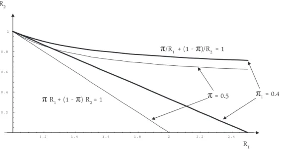
Condition (22) with 1 = is the converse of the condition that ensures
interim Pareto optimality of the competitive equilibrium (1). As expected, when the bubbleless equilibrium is not interim Pareto optimal, there exists a bubbly equilibrium. Figure 4 gives an illustration of the di¤erent cases depending on the values of R1 and R2: The curves are drawn for the value
= 1=2:
The case of pessimism
Agents are assumed to be pessimistic: 1 < : If
1 <
R1(1 R2)
R1 R2
a deterministic bubble exists in an economy in which there would be no bubble if agents did not "transform" the probabilities. The interpretation of this result is simple. Investing in the bubble provides a gross return equal to 1; which is greater than the capital return in the bad state of the nature R2:
Agents invest in the bubble in order to be protected against the occurrence of state 2. In the case of pessimism, they put more weight on this state and invest more in the bubble. Therefore, pessimism can play in favor of the existence of a deterministic bubble. From Proposition 2, a bubbly equilibrium can only exist in an ine¢cient economy.
Figure 5 gives an illustration of the e¤ect of pessimism on the existence of the di¤erent regimes in the plane (R1; R2): The curves are obtained under the
assumption that the pessimism generates a transformation of from = 1=2 to 1 = 0:4:
The case of optimism
The condition ensuring the existence of a bubbly equilibrium remains Con-dition (22). Optimism is unfavorable to the existence of bubbles, as agents put more weight on the good state of the nature.
The relation between the existence of bubbles and interim Pareto opti-mality is more complex in the case of optimism. The usual way to analyze the impact of a bubble is to interpret it as an intergenerational transfer. In the basic economy with standard EU preferences, when (9) is not ful…lled, the existence of a bubble constitutes an intergenerational transfer from the young to the old agents and this transfer is Pareto improving. This analysis can also be used to understand the case of pessimistic agents. But, with opti-mistic agents, preferences are no longer convex. If (12) holds and (13) is not ful…lled, it may be possible that the economy is not interim Pareto optimal and that no bubbly equilibrium exists. Considering the proof of Proposi-tion 3, the competitive equilibrium without bubbles can be ine¢cient in this case, because the technology does not allow agents to redistribute consump-tion from state 1 in favor of state 2. A deterministic bubble cannot solve this problem as the bubble carries out a transfer among generations, and not a transfer among the two states of nature.
3.2
Equilibrium with a stochastic bubble
In this part, a stochastic bubble à la Weil (1987) is introduced. Following Weil, the asset has some probability to explode at each period. More pre-cisely, agents form their expectations according to a self-ful…lling prophecy which assumes that the bubble will continue if some state of the nature oc-curs, and will burst if the other state arises. In all the section, we assume that the continuation of the bubble is conditional to the realization of state 2; and that the bubble bursts if state 1 occurs. This assumption is taken be-cause it is the most favorable to the existence of the bubble. Indeed, agents can arbitrate between the two assets, the productive capital and the bubbly asset. Investing in the stochastic bubble allows to be insured against the occurrence of the state with a low return of productive capital. It would be impossible to have a stochastic bubble which existence is conditional to state 1: This asset would be dominated by productive capital, or its value should grow at a factor greater than R1: This last case would be unsustainable.
3.2.1 The bubble à la Weil (1987)
A bubble asset à la Weil (1987) is available in the economy in a …xed quantity normalized to 1: Its price is pt in period t; conditional to the realization of
state 2. Assuming that the economy is in period t in state 2, agents expect a price pt+1 in period t + 1 conditional to the realization of state 2, and a price
0 if state 1 occurs. In the case of the bubble exploding, the dynamics of the economy after the explosion becomes the same as in the economy without the bubble.
Assuming that state 2 occurs in period t; the budget constraints of a generation t agent are:
ct+ st+ ptxt = w (24)
d1t+1 = R1st (25)
d2t+1 = R2st+ pt+1xt (26)
in-tertemporal budget constraint: ct+ d1 t+1 R1 1 R2 pt pt+1 + d2t+1 pt pt+1 = w (27)
3.2.2 Stochastic bubbles in the EU model
In the EU model, an agent maximizes (4) under budget constraints (24), (25) and (26). The results are:
ct = w 1 + st = w 1 + 1 ptR2 pt+1 xt = w 1 + (1 ) pt R2 pt+1 ptR2
Equilibrium conditions on the bubble market (xt= 1) and on the capital
market Kt= st imply: 1 = w 1 + (1 ) pt R2 pt+1 ptR2 (28) Kt = w 1 + 1 ptR2 pt+1 (29)
With the change of variable t= pt(1 + )=( w); equation (28) gives:
t+1 = R2 t
1 t
1 t
This equation has 2 stationary states: 0 which is stable, and
= 1 R2 1 R2
which is unstable. This last steady state exists only if > 0,
R2 < 1 (30)
Proposition 5 If condition (30) holds, there exists an equilibrium of the economy associated with a stochastic bubble conditional to the continuation of state 2.
This condition is stronger than (22): the deterministic bubble is more likely to exist than the stochastic bubble. Indeed, the stochastic bubble has a positive return only if state 2 arises. Moreover, the stochastic bubble cannot exist in an e¢cient economy: if (30) holds, (9) does not hold. A graphical illustration of these results is shown in Figure 4, with a value = 1=2:
As for the case of deterministic bubbles, when (30) holds, there exists a multiplicity of equilibria: either the economy stays at the bubbly steady state; either the economy stays at the bubbleless equilibrium; or, starting from a value 0 < ; the economy converges towards the bubbleless stationary
equilibrium.
3.2.3 Two types of bubbly equilibria in the RDU model
A stochastic bubble conditional to state 2 may induce some redistribution of consumption between the two states of nature. For the equilibrium with a deterministic bubble, state 1 always remains the best state of the nature. For an equilibrium with a stochastic bubble conditional to state 2, it is possible that state 2 becomes the good state of the nature, as the bubble bursts in state 1. More precisely, the size of the bubble may determine which is the best state. For a small bubble, state 1 will always lead to more consumption than state 2. For a large bubble, the inequality can be reversed. Therefore, it is a priori possible to obtain two types of bubbly equilibria, associated either with d2 < d1 or with d2 > d1:
Equilibrium such that d2 > d1
Assuming that the equilibrium is such that d2
t+1 > d1t+1; the program of
the agent consists in maximizing (6) under the three budget constraints (24), (25) and (26). The results are:
ct = w 1 + st = w 1 + 2 1 ptR2 pt+1 xt = w 1 + (1 2) pt 2R2 pt+1 ptR2
The equilibrium condition on the bubble market (xt = 1) leads to the
dy-namics of the price of the bubble. Using the variable t= pt(1 + )=( w); t
follows the dynamic equation:
t+1 = R2 t 1 t 1 2 t (31) The condition d2 t+1 = R2st+ pt+1 > d1t+1 = R1st leads to: t+1 > R2 t+ (R1 R2) 2
With (31), this condition gives:
t>
R1 R2
R1
(1 2) ^l (32)
The bubble must be large enough to change the ranking of the states 1 and 2.
The bubbly steady state corresponds to
^ = 1 2 R2
1 R2
It exists only if ^ > 0 or
2 < 1 R2 (33)
Moreover, condition (32) must be checked along this equilibrium. It leads to the constraint:
2 <
1 R2
R1+ 1 R2
(34)
This last condition is stronger than (33) as R1+ 1 R2 > 1.
Equilibrium such that d2 < d1
Assuming that the equilibrium is such that d2
t+1 < d1t+1; the program of
the agent gives:
ct = w 1 + st = w 1 + 1 1 ptR2 pt+1 xt = w 1 + (1 1) pt 1R2 pt+1 ptR2
The equilibrium condition on the bubble market (xt = 1) leads to the
dy-namics of the price of the bubble. The variable t = pt(1 + )=( w) follows
the dynamic equation:
t+1 = R2 t 1 t 1 1 t (35) The condition d2 t+1 = R2st+ pt+1 < d1t+1 = R1st leads to: t+1 < R2 t+ (R1 R2) 1
With (35), this condition gives:
t<
R1 R2
R1
(1 1) l (36)
In this case, the value of the bubble must be low enough to not change the ranking of the states.
The bubbly steady state corresponds to
= 1 1 R2 1 R2
It exists only if > 0:
1 < 1 R2 (37)
Moreover, must satisfy (36):
1 >
1 R2
R1+ 1 R2
(38)
The case of a stochastic bubble associated with RDU preferences leads to new results that could not occur in the standard EU framework. The RDU framework gives birth to two types of bubbly equilibria associated with either a low price or a high price for the bubble. These results come from the property that the weights put on the di¤erent states of the nature depend on the rank within the RDU framework. A stochastic bubble with a low value does not change the ranking of the two states of the nature whereas a bubble with a high value does.
3.2.4 Stochastic bubbles and optimism
For an optimistic agent, 1 > > 2; and thus, ^ > : Depending on the
value of the parameters, it is possible to obtain a bubbly equilibrium with d1 < d2 and a high price level of the bubble, or a bubbly equilibrium with
d1 > d2 and a low price level of the bubble.5 The following propositions (6, 7
and 8) show that, for given values of parameters, only one type of equilibrium is possible, either associated with d1 < d2 , or with d1 > d2:
Using conditions (33), (34) , (37) and (38), the following results are ob-tained.
Proposition 6 Assume that 2 < R11 R+1 R2 2 and 1 > 1 R2or 1 < R11 R+1 R2 2:
There exists a unique bubbly equilibrium with d1 < d2 and a price of the bubble
equal to ^( w)=(1 + ):
Proposition 6 shows that optimism can play in favor of the existence of bubbles. Assume that > 1 R2: Under this condition, stochastic bubbles
cannot exist in the economy with EU preferences. If agents are optimistic, it is possible that they transform probabilities with 2 = 1 (1 ) < R11 R+1 R2 2:
In this case a stochastic bubble may exist. The price of the bubble is high enough in such a way that consumption in state 2 (the bubble exists) is higher than consumption in state 1 (the bubble explodes). As agents are optimistic, they put more weight on the good state and invest more in the bubble.
Proposition 7 corresponds to the converse case of a low price of the bubble such that d1 remains higher than d2:
Proposition 7 Assume that 1 < 1 R2 and 2 > R11 R+1 R2 2: There exists
a unique bubbly equilibrium with d1 > d2 and a price of the bubble equal to
( w)=(1 + ):
As < 1 < 1 R2; a necessary condition for the existence of such
an equilibrium is that there exists a bubbly equilibrium in the economy with
5It is not possible to obtain a bubbly equilibrium such that d1=d2;because it is never
EU preferences (see condition (30)). Moreover agents need to be not too opti-mistic, in such a way that 1and 2remain in the interval R11 R+1 R2 2; 1 R2 :
A last case remains to be studied, if
2 <
1 R2
R1+ 1 R2
< 1 < 1 R2
In this case, all preceding conditions (33), (34) , (37) and (38) are ful…lled. But, it does not imply that the two types of bubbly equilibria can exist together. Indeed, in the case of optimistic agents, preferences are not convex. It is possible that two di¤erent solutions satisfy the marginal conditions of the consumer program, one with d1 < d2, the other one with d1 > d2: Therefore,
it is necessary to compare the utility levels associated with the two solutions. This is done in the following proposition.
Proposition 8 Assume that 2 < R11 R+1 R2 2 < 1 < 1 R2: The function
is de…ned according to:
( ) = ln R1 1 R2
+ (1 ) ln(1 )
If ( 2) > ( 1) then a bubbly equilibrium with d1 < d2 exists and the
price of the bubble is equal to ^( w)=(1 + ):
If ( 2) < ( 1) then a bubbly equilibrium with d1 > d2 exists and the
price of the bubble is equal to ( w)=(1 + ):
Proof. See Appendix 5.
To summarize the impact of optimism on the existence of stochastic bub-bles, the most interesting result is obtained in Proposition 6. Optimism may favor stochastic bubbles with respect to EU preferences. The price of the bubble must be high enough in such a way that d1 < d2: In that case, state 2
(the bubble exists) can be better than state 1 (the bubble bursts). Optimistic agents put more weight on the good state and invest more in the bubble.
In overlapping generations models à la Tirole (1985), there exists a max-imum size of the bubble that corresponds to the saddle path converging towards the long run bubbly steady state. There also exists a multiplicity of equilibria starting with a value of the bubble between 0 and the maximum
value. All these equilibria converge towards the long run bubbleless equilib-rium. In our model with RDU preferences and a stochastic bubble, it is possible that these properties are no more satis…ed. Under the assumptions of proposition (6), there exists a stationary bubbly equilibrium with a price of the bubble equal to ^( w)=(1 + ): But any initial value below the steady state value is not admissible. For an optimistic agent, as 1 > 2; the two
constraints (32) and (36) are such that ^l > l: Therefore, any initial value 0 such that l < 0 < ^l is not admissible as it cannot correspond to an
equilibrium path.6
3.2.5 Stochastic bubbles and pessimism
For a pessimistic agent, 1 < < 2: Using conditions (33), (34), (37) and
(38), it is possible to obtain existence conditions for the bubbly equilibria that satisfy the marginal conditions of the consumer program, as in Propositions 6 and 7.7 But, in the case of pessimism, another situation may exist that
corresponds to d1
t+1 = d2t+1. This case results from the existence of a kink for
d1
t+1 = d2t+1:
Considering the maximization of the RDU function under the intertempo-ral budget constraint (27), the optimal solution with d1
t+1 = d2t+1 is obtained if: 1 1 1 < 1 R2 pt pt+1 R1pt+1pt < 2 1 2 (39)
It corresponds to the solution:
ct = w 1 + d1t+1 = d2t+1 = w 1+ 1 R1 R2 R1 pt pt+1 + pt pt+1
The equilibrium price of the bubble satis…es:
pt = w 1 + pt pt+1(R1 R2) 1 + pt pt+1(R1 R2)
6I am grateful to an anonymous referee that has pointed out this property.
7The case studied in Proposition 8 does no more exist as it was related to the non
With the change of variable t= pt(1 + )=( w); this equation gives:
t = 0 or
t+1 = t(R1 R2) + (R1 R2) (40)
(40) has a stationary state
~ = R1 R2
1 + R1 R2
If R1 R2 > 1; this stationary state is unstable. If R1 R2 < 1; it is stable. In
this case, it is possible to observe convergence towards the stationary state, with oscillations. In the case of instability, there is only one stationary bubbly equilibrium. In the case of stability, a multiplicity of bubbly equilibria exists. Finally, the following results have been obtained in the case of a pes-simistic agent:
Proposition 9 Assume that 1 < < 2:
If
2 <
1 R2
R1+ 1 R2
a bubbly equilibrium with d1 < d2 exists and the price of the bubble is
equal to ^( w)=(1 + ):
If
1 R2
R1+ 1 R2
< 1 < 1 R2
a bubbly equilibrium with d1 > d2 exists and the price of the bubble is
equal to ( w)=(1 + ): If 1 < 1 R2 R1+ 1 R2 < 2
a stationary bubbly equilibrium exists associated with a price of the bubble ~( w)=(1 + ):
- If R1 R2 < 1; it is stable. In this case, a multiplicity of bubbly
equilibria exists that converge towards the steady state with oscil-lations.
To summarize, pessimism may favor stochastic bubbles such that d1 >
d2 with respect to EU preferences. To illustrate this point, assume that
> 1 R2: Under this condition, stochastic bubbles cannot exist in the
economy with EU preferences. If agents are pessimistic, it is possible that they transform probabilities in such a way that 1 = ( ) < 1 R2: In this
case a stochastic bubble can exist. The price of the bubble is low enough in such a way that consumption in state 2 (the bubble exists) remains lower than consumption in state 1 (the bubble explodes). As agents are pessimistic, they put more weight on the bad state and invest more in the bubble.
The previous section has showed that optimism may favor stochastic bub-bles with a high enough price in such a way that d1 < d2: This section proves
that pessimism may favor stochastic bubbles with a low price. Therefore, the same parameter (the degree of optimism) can have opposite e¤ects depend-ing on the type of the bubble. This result comes from the property that the weights put on the di¤erent states of the nature depend on the rank within the RDU framework. A stochastic bubble with a low value does not change the ranking of the two states of the nature whereas a bubble with a high value does. In the …rst case, pessimism favors the existence of the bubble whereas optimism favors the existence of the bubble in the second case.
Moreover it is possible to have indeterminacy with a multiplicity of bubbly equilibria converging towards a steady state with oscillations. This result of indeterminacy is related to the existence of a kink on the indi¤erence curves for d1 = d2. When d1 = d2; it is possible that di¤erent values of
the price of the bubble are compatible with an equilibrium. Indeterminacy results from the RDU assumption, but is also related to the assumption of a linear production technology. It is possible to check that indeterminacy vanishes in the case of a Cobb-Douglas technology that eliminates the impact of uncertainty on dynamic ine¢ciency. Indeterminacy needs a high enough elasticity of substitution.
Choquet utility has been obtained in other frameworks: Tallon (1997) and Epstein and Wang (1994) also obtain this result in models of …nancial assets.
4
Conclusion
This paper has proposed a simple model that suggests that uncertainty as-sociated with RDU preferences can extend the scope for the existence of rational …nancial bubbles. Pessimism favors the existence of deterministic bubbles, when optimism may promote the existence of stochastic bubbles. Moreover, associated with pessimism, the RDU assumption is a new cause of multiple bubbly equilibria.
It would be interesting to expand these …rst results into a more gen-eral framework. A …rst improvement would consist in introducing di¤erent production technologies subject to di¤erent shocks, with many states of the nature. Considering non-linear production technologies could also be an in-teresting generalization.
Another development would be to assume heterogeneous agents di¤ering by their degree of pessimism or optimism.
References
[1] Abel, A.B., Mankiw, N.G., Summers L.H., Zeckhauser R.J., 1989. As-sessing dynamic e¢ciency: theory and evidence. Review of Economic Studies 56(1), 1-19.
[2] Allais, M., 1947. Economie et Intérêt, ed. Imprimerie Nationale.
[3] Allais, M., 1953. Le comportement de l’homme rationnel devant le risque: critique des postulats et axiomes de l’école Américaine. Econo-metrica 21(4), 503–546.
[4] Blanchard, O.J., Weil, P., 2001. Dynamic e¢ciency, the riskless rate, and debt Ponzi games under uncertainty. The B.E. Journal of Macro-economics 1(2), 1-23.
[5] Bosi, S., Seegmuller, T., 2010. On rational exuberance. Mathematical Social Sciences, 59(2), 249-270.
[6] Boswijk, H.P., Hommes, C.H., Manzan, S., 2007. Behavioral hetero-geneity in stock prices. Journal of Economic Dynamics and Control 31, 1938-1970.
[7] Brock, W.A., Hommes, C.H., Wagener, F.O.O., 2009. More hedging instruments may destabilize markets. Journal of Economic Dynamics and Control 33, 1912-1928.
[8] Caballero, R.J., Hammour, M.L., 2002. Speculative growth. NBER Working Papers 9381, National Bureau of Economic Research, Inc.
[9] Caballero, R.J., Farhi, E., Hammour, M., 2006. Speculative growth: hints from the U.S. economy. American Economic Review 96(4), 1159-1192.
[10] Cass, D., 1972. On capital overaccumulation in the aggregative, neoclas-sical model of economic growth: a complete characterization. Journal of Economic Theory 4, 200-223.
[11] Chateauneuf, A. 1999. Comonotonicity axioms and RDU theory for ar-bitrary consequences. Journal of Mathematical Economics 32, 21-45.
[12] Cohen, M., Tallon, J. M. 2000. Décision dans le risque et l’incertain: l’apport des modèles non-additifs. Revue d’Economie Politique 110(5), 631-681.
[13] De La Croix, D., Michel, P., 2002. A theory of economic growth: dynam-ics and policy in overlapping generations, Cambridge University Press.
[14] Demange, G., Laroque, G., 1999. Social security and demographic shocks. Econometrica 67(3), 527-542
[15] Diamond, P., 1965. National debt in a neoclassical growth model. Amer-ican Economic Review 55(5), 1126–1150.
[16] Dow, J., da Costa Werlang, S.R., 1992. Excess volatility of stock prices and Knightian uncertainty. European Economic Review, 36(2-3), 631-638.
[17] Epstein, L.G., Wang, T., 1994. Intertemporal asset pricing under Knightian uncertainty. Econometrica 62(2), 283-322.
[18] Farhi, E., Tirole, J., 2008. Competing liquidities: corporate securities, real bonds and bubbles. NBER Working Paper No. 13955.
[19] Farhi, E., Tirole, J., 2012. Bubbly liquidity. Review of Economic Studies 79(2), 678-706.
[20] Gottardi, P., 1996. Stationary monetary equilibria in overlapping gen-erations models with incomplete markets. Journal of Economic Theory 71, 75-89.
[21] Grossman, G., Yanagawa, N., 1993. Asset bubbles and endogenous growth. Journal of Monetary Economics 31(1), 3-19.
[22] Homburg, S., 1992. E¢cient Economic Growth, Springer, Berlin usw.
[23] Hommes, C.H., 2006. Heterogeneous agent models in economics and …-nance, in: Tesfatsion L., Judd, K.L. (Eds), Handbook of Computational Economics, Volume 2: Agent-Based Computational Economics, Elsevier Science B.V., pp. 1109-1186.
[24] Hommes, C.H., Sonnemans, J., Tuinstra, J., van de Velden, H., 2008. Expectations and bubbles in asset pricing experiments. Journal of Eco-nomic Behavior & Organization 67, 116-133.
[25] Kindleberger, C.P., Aliber, R.Z., 2011. Manias, Panics and Crashes: a History of Financial Crises, Palgrave Macmillan , 6th ed, New York.
[26] Machina, M.J., 1989. Dynamic consistency and non-expected utility models of choice under uncertainty. Journal of Economic Literature 27(4), 1622-1668.
[27] Martin, A., Ventura, J., 2012. Economic growth with bubbles. American Economic Review 102 (6), 3033-3058.
[28] Minsky, H.P., 1982. The …nancial instability hypothesis: capitalistic processes and the behavior of the economy, in: Kindleberger, C.P., La¤argue, J.P. (Eds), Financial Crises: Theory, History, and Policy. Cambridge University Press, Cambridge, pp. 12-29.
[29] Olivier, J., 2000. Growth-enhancing bubbles. International Economic Review 41(1), 133-151.
[30] Peled, D., 1984. Stationary pareto optimality of stochastic asset equi-libria with overlapping generations. Journal of Economic Theory 34, 396-403.
[31] Peled, D., Aiyagari, R., 1991. Dominant root characterization of Pareto optimality and the existence of optimal equilibria in stochastic overlap-ping generations models. Journal of Economic Theory 54, 69-83.
[32] Quiggin, J., 1982. A theory of anticipated utility. Journal of Economic Behavior and Organisation 3, 323–343.
[33] Samuelson, P., 1958. An exact consumption-loan model of interest with or without the social contrivance of money. Journal of Political Economy 66, 467-482.
[34] Tallon, J.M., 1997. Risque microéconomique et prix d’actifs dans un modèle d’équilibre général avec espérance d’utilité dépendante du rang Finance. Revue de l’Association Française de Finance 18, 139-153.
[35] Tirole, J., 1985. Asset bubbles and overlapping generations. Economet-rica 53(6), 1499-1528.
[36] Wang, Y., 1993. Stationary equilibria in an overlapping generations economy with stochastic production. Journal of Economic Theory 61, 423-435.
[37] Weil, P., 1987. Con…dence in the real value of money in an overlapping generations economy. Quarterly Journal of Economics 52(1), 1-22.
[38] Wigniolle, B., 2012. Optimism, pessimism and …nancial bubbles. Docu-ments de travail du Centre d’Economie de la Sorbonne 12005, Université Paris 1 Panthéon-Sorbonne, Centre d’Economie de la Sorbonne.
[39] Zilcha, I., 1991. Characterizing e¢ciency in stochastic overlapping gen-erations models. Journal of Economic Theory. 55(1), 1-16.
5
Appendixes
5.1
Appendix 1: proof of Proposition 1.
The proof uses the method developed by Homburg (1992) and De la Croix and Michel (2002). Some notations are introduced. ht denotes a particular
history from period 0 till t (the state 0at period 0 is assumed to be known in
t = 0): ht= ( 0; 1; 2; :::; t): Ht is the set of all possible t-period histories
from period 0: #Ht = 2t as 0 is known in 0. The applications and
are de…ned such that, for an history ht = ( 0; 1; 2; :::; t 1; t) 2 Ht;
(ht) = ( 0; 1; 2; :::; t 1) and (ht) = t:
The allocation corresponding to the competitive equilibrium is such that, for all t 0: K 1 is given, d0 = R( 0)K 1; ct = 1+w c; Kt = 1+w K;
dt+1 = R(1+t+1) w:Using the following notation, d( t) = R(1+t) w; the
corre-sponding ex-ante utility level is: U ln (c)+ ln d(1) + (1 ) ln d(2) : Assuming that this allocation is not interim Pareto optimal means that there exists another feasible allocation that, almost surely, gives a higher expected utility for all period t with a strict improvement on a set of states of positive measure. Formally, it means that it is possible to …nd an allocation (~c(ht); ~d(ht); ~K(ht))ht2Ht; t 0 such that 8t
~
c(ht) + ~d(ht) + ~K(ht) = R( (ht)) ~K( (ht)) + w
~
K ( (h0)) = K 1 (initial condition given)
(feasibility), and such that 8t; 8ht2 Ht
ln (~c(ht)) + ln ~d((ht; 1)) + (1 ) ln ~d((ht; 2)) U (41)
~
with a strict inequality for some ht0:
First, it is easy to check that the competitive solution (c; d(1); d(2)) in period t can be obtained through the following program:
max (c;d1;d2)ln (c) + ln d 1 + (1 ) ln d2 s.t. w = c + R1 d1+(1 ) R2 d2
As a consequence of this property, (41) implies that, 8t; 8ht2 Ht
~ c(ht) + R1 ~ d((ht; 1)) + (1 ) R2 ~ d((ht; 2)) c + R1 d(1) + (1 ) R2 d(2)
with a strict inequality for some history ht0:
For a state t; t 2 f1; 2g ; the function is de…ned as: (1) = and
(2) = 1 : For an history ht = ( 0; 1; 2; :::; t 1; t) 2 Ht; P (ht) is de…ned as P (ht) = t Q i=1 ( i) t Q i=1 R( i) and P ( 0) = 1: Therefore, P (ht) = ( (ht)) R( (ht)) P ( (ht))
For T > t0; it is obtained that ~d( 0) d0+ T 1 P t=0 P ht2Ht P (ht) ~c(ht) + R1 ~ d((ht; 1)) + (1 ) R2 ~ d((ht; 2)) c R1 d(1) (1 ) R2 d(2) > 0
Rearranging the terms that depend on the same period, the following is obtained: T 1 P t=0 P ht2Ht P (ht) h ~ c(ht) + ~d(ht) c d( (ht)) i + P hT2HT P (hT)h ~d((hT)) d( (hT)) i > 0
From the feasibility constraints, it is obtained:
T 1 P t=0 P ht2Ht P (ht) h R( (ht)) ~K( (ht)) K(h~ t) R( (ht))K + K i + P hT2HT P (hT)h ~d((hT)) d( (hT)) i > 0
After simpli…cations, it is obtained: P hT 12HT 1 P (hT 1) h ~ K(hT 1) + K i + P hT2HT P (hT)h ~d((hT)) d( (hT)) i > 0 (43) It is possible to write: ~ K(hT 1)+K = R(1)R(1) h ~ K(hT 1) + K i +1 R(2)R(2) h ~ K(hT 1) + K i
Replacing in (43) makes it possible to write: P
hT2HT
P (hT)h ~d(hT) R( (hT)) ~K ( (hT)) d( (hT)) + R( (hT))K
i > 0
Using the feasibility constraint leads to: P hT2HT P (hT) h c + K ~c(hT) K (h~ T) i > 0
Finally, c + K = w and it is obtained: " P hT2HT P (hT) # w > P hT2HT P (hT) h c + K ~c(hT) K (h~ T) i > 0
Introducing the notation ST =
P
hT2HT
P (hT)
it is straightforward to check that
ST = R1 + 1 R2 ST 1 Therefore, if R 1 + 1
R2 < 1; limT !1ST = 0 and the competitive equilibrium is
interim Pareto-optimal.
5.2
Appendix 2: proof of Proposition 2.
The proof is adapted from the preceding one, replacing by 1. The
com-petitive solution in period t can be obtained through the following program:
max (c;d1;d2)ln (c) + 1ln d 1 + (1 1) ln d2 s.t. w = c + 1 R1 d1+(1 1) R2 d2
As the agent is pessimistic, its preferences remain strictly convex. There-fore, the preceding reasoning can be used: a feasible allocation (~c(ht); ~d(ht);
~
K(ht))ht2Ht; t 0 that interim Pareto-dominates the competitive equilibrium
must satisfy 8t; 8ht2 Ht ~ c(ht) + 1 R1 ~ d((ht; 1)) + (1 1) R2 ~ d((ht; 2)) c + 1 R1 d(1) + (1 1) R2 d(2)
with a strict inequality for some history ht0: Thereafter, the proof is the same,
replacing by 1:
5.3
Appendix 3: proof of Proposition 3.
The proof is adapted from Appendix 1. The competitive solution in period t can be obtained through the following program:
max (c;d1;d2)ln (c) + 1ln d 1 + (1 1) ln d2 s.t. w = c + 1 R1 d1+(1 1) R2 d2
But, as the agent is optimistic, its preferences are no more convex. More precisely, it is possible that the program
max (c;d1;d2)ln c + E ln(d) (44) s.t. w = c + 1 R1 d1+ (1 1) R2 d2
has its optimal solution in the domain d1 < d2: In this case the solution
results from the program
max (c;d1;d2)ln (c) + 2ln d 1 + (1 2) ln d2 s.t. w = c + 1 R1 d1+(1 1) R2 d2
The solution is:
c = w 1+ d 1 = 2 1 R1 w 1+ d 2 = 1 2 1 1 R2 w 1+