HAL Id: hal-02864992
https://hal.archives-ouvertes.fr/hal-02864992
Submitted on 11 Jun 2020
HAL is a multi-disciplinary open access
archive for the deposit and dissemination of
sci-entific research documents, whether they are
pub-lished or not. The documents may come from
teaching and research institutions in France or
abroad, or from public or private research centers.
L’archive ouverte pluridisciplinaire HAL, est
destinée au dépôt et à la diffusion de documents
scientifiques de niveau recherche, publiés ou non,
émanant des établissements d’enseignement et de
recherche français ou étrangers, des laboratoires
publics ou privés.
water stable isotope records from a highly resolved firn
core from Adélie Land, coastal Antarctica
Sentia Goursaud, Valérie Masson-Delmotte, Vincent Favier, Susanne
Preunkert, Michel Legrand, Bénédicte Minster, Martin Werner
To cite this version:
Sentia Goursaud, Valérie Masson-Delmotte, Vincent Favier, Susanne Preunkert, Michel Legrand, et
al.. Challenges associated with the climatic interpretation of water stable isotope records from a
highly resolved firn core from Adélie Land, coastal Antarctica. The Cryosphere, Copernicus 2019, 13,
pp.1297 - 1324. �10.5194/tc-13-1297-2019�. �hal-02864992�
https://doi.org/10.5194/tc-13-1297-2019
© Author(s) 2019. This work is distributed under the Creative Commons Attribution 4.0 License.
Challenges associated with the climatic interpretation of water
stable isotope records from a highly resolved firn core from
Adélie Land, coastal Antarctica
Sentia Goursaud1,2, Valérie Masson-Delmotte1, Vincent Favier2, Suzanne Preunkert2, Michel Legrand2, Bénédicte Minster1, and Martin Werner3
1LSCE (UMR CEA-CNRS-UVSQ 8212-IPSL), Gif-sur-Yvette, France 2Univ. Grenoble Alpes, CNRS, IGE, 38000 Grenoble, France
3Alfred Wegener Institute, Helmholtz Centre for Polar and Marine Research, Bremerhaven, Germany
Correspondence: Sentia Goursaud (sentia.goursaud@lsce.ipsl.fr) Received: 7 June 2018 – Discussion started: 4 July 2018
Revised: 12 March 2019 – Accepted: 14 March 2019 – Published: 24 April 2019
Abstract. A new 21.3 m firn core was drilled in 2015 at a coastal Antarctic high-accumulation site in Adélie Land (66.78◦S; 139.56◦E, 602 m a.s.l.), named Terre Adélie 192A (TA192A).
The mean isotopic values (−19.3 ‰ ± 3.1 ‰ for δ18O and 5.4 ‰±2.2 ‰ for deuterium excess) are consistent with other coastal Antarctic values. No significant isotope–temperature relationship can be evidenced at any timescale. This rules out a simple interpretation in terms of local temperature. An observed asymmetry in the δ18O seasonal cycle may be ex-plained by the precipitation of air masses coming from the eastern and western sectors in autumn and winter, recorded in the d-excess signal showing outstanding values in aus-tral spring versus autumn. Significant positive trends are ob-served in the annual d-excess record and local sea ice extent (135–145◦E) over the period 1998–2014.
However, process studies focusing on resulting isotopic compositions and particularly the deuterium excess–δ18O re-lationship, evidenced as a potential fingerprint of moisture origins, as well as the collection of more isotopic measure-ments in Adélie Land are needed for an accurate interpreta-tion of our signals.
1 Introduction
1.1 Motivation for new coastal Antarctic firn cores Polar ice cores are exceptional archives of past climate variations. In Antarctica, many deep ice cores have been drilled and analysed since the 1950s. For instance, Stenni et al. (2017) compiled water stable isotope data from 112 ice cores spanning at least part of the last 2000 years. Most deep ice cores were drilled in the central Antarctic plateau where low accumulation rates and ice thinning give access to long climate records. In today’s context of rapid global climate change, it is of paramount importance to also docu-ment recent past climate variability around Antarctica. Many Antarctic regions still remain undocumented due to the lack of accumulation and water stable isotope records from shal-low ice cores or pits (Jones et al., 2016; Masson-Delmotte et al., 2008). An accurate knowledge of changes in coastal Antarctic surface mass balance (SMB), an evaluation of the ability of climate models to resolve the key processes affect-ing its variability, and thus an improved confidence in pro-jections of future changes in coastal Antarctic surface mass balance are important to reduce uncertainties on the ice sheet mass balance and its contribution to sea level change (Church et al., 2013).
Meteorological observations have been conducted since 1957 in manned and automatic stations (Nicolas and Bromwich, 2014), and considerable efforts have been de-ployed to compile and update the corresponding dataset
(Turner et al., 2004). This network is marked by gaps in spatio-temporal coverage (Goursaud et al., 2017) as well as systematic biases of instruments such as thermistors (Gen-thon et al., 2011). Satellite remote-sensing data have been available since 1979 and provide large-scale information for changes in Antarctic sea ice and temperature (Comiso et al., 2017), but do not provide sufficient accuracy and homogene-ity to resolve trends at local scales (Bouchard et al., 2010). Coastal shallow (20–50 m long) firn cores are thus essential to provide continuous climate information spanning the last decades at sub-annual resolution, at local but also regional scales. They complement stake area observations of spatio-temporal variability in surface mass balance (Favier et al., 2013), which also help assess the representativeness of a sin-gle record.
Since the 1990s, efforts have been made to retrieve shal-low ice cores in coastal Antarctic areas. Most of these efforts have been focused on the Atlantic sector, in Dronning Maud Land (Altnau et al., 2015; Graf et al., 2002; e.g. Isaksson and Karlén, 1994) and the Weddell Sea sector (Mulvaney et al., 2002). Fewer annually resolved water stable isotope records have been obtained from ice cores in other regions, such as the peninsula (Fernandoy et al., 2018), the Ross Sea sector (Bertler et al., 2011), Law Dome (Masson-Delmotte et al., 2003; Delmotte et al., 2000; Morgan et al., 1997), Adélie Land (Yao et al., 1990; Ciais et al., 1995; Goursaud et al., 2017), and the Princess Elizabeth region (Ekaykin et al., 2017). However, the recent 2000-year temperature and SMB reconstructions for the Antarctic (Stenni et al., 2017; Thomas et al., 2017) highlighted the need for more coastal records. In this line, new drilling efforts have recently been initiated in the context of the ASUMA project (Improving the Accuracy of SUrface Mass balance of Antarctica) from the French Agence Nationale de la Recherche, which aims to assess spatio-temporal variability and change in SMB over the transition zone from coastal Adélie Land to the central East Antarctic Plateau (towards Dome C).
1.2 Climatic interpretation of water stable isotope records
Water stable isotope (δ18O, δD) records from central Antarc-tic ice cores have classically been used to infer past tem-perature changes (e.g. Jouzel et al., 1987). The isotope– temperature relationship was nevertheless shown not to be stationary and to vary in space (Jouzel et al., 1997), calling for site-specific calibrations relevant for various timescales (Stenni et al., 2017). In coastal regions, several studies showed no temporal isotope–temperature relationship at all between water stable isotope records in firn cores covering the last decades and near-surface air temperature measured at the closest station. This is for instance the case in Dron-ning Maud Land, near the Neumayer station (three firn cores, for which the longest covered period is 1958–2012; Vega et al., 2016), in the Ross Sea sector (one snow pit covering
the period 1964–2000; Bertler et al., 2011), and in Adélie Land, close to Dumont d’Urville (DDU, one firn core cover-ing the period 1946–2006; Goursaud et al., 2017). While sev-eral three-dimensional atmospheric modelling studies have suggested a dominant role of large-scale atmospheric circu-lation in the variability of coastal Antarctic snow δ18O (e.g. Noone, 2008; Noone and Simmonds, 2002), understanding the drivers of coastal Antarctic δ18O variability remains chal-lenging (e.g. Fernandoy et al., 2018; Bertler et al., 2018; Schlosser et al., 2004; Dittmann et al., 2016). While distil-lation processes are expected theoretically to relate conden-sation temperature with precipitation isotopic composition, a number of deposition processes can distort this relation-ship: changes in moisture sources (Stenni et al., 2016), inter-mittency or seasonality of precipitation (Sime et al., 2008), boundary layer processes affecting the links between con-densation and surface air temperature (Krinner et al., 2008), and several post-deposition processes, such as the effects of winds (Eisen et al., 2008), snow–air exchanges (Casado et al., 2016; Ritter et al., 2016), and diffusion processes in snow and ice (e.g. Johnsen, 1977). Nevertheless, all these processes remain poorly quantified. As a result, comparisons between firn core records with precipitation records or simu-lations have to be performed carefully.
Changes in the atmospheric water cycle can also be in-vestigated using a second-order parameter, deuterium excess (excess). The definition given by Dansgaard (1964) as d-excess = δD–8× δ18O aims to remove the effect of equilib-rium fractionation processes to identify differences in kinetic fractionation between the isotopes of hydrogen and oxygen. In Antarctica, spatial variations in d-excess have been docu-mented through data syntheses, showing an increase from the coast to the plateau (Masson-Delmotte et al., 2008; Touzeau et al., 2016), but temporal variations in d-excess (seasonal cycle, inter-annual variations) remain poorly documented and understood.
Theoretical isotopic modelling studies show that d-excess depends on evaporation conditions, mainly through the im-pacts of relative humidity (RH) and sea surface temperature (SST) on kinetic fractionation at the moisture source (Merli-vat and Jouzel, 1979; Petit et al., 1991; Ciais et al., 1995), and the preservation of the initial vapour signal during transporta-tion towards polar regions (e.g. Jouzel et al., 2013; Bonne et al., 2015). The effect of wind speed on kinetic fractionation is secondary and thus has been neglected in climatic inter-pretations of d-excess. Some studies usually privileged one variable (RH or SST). For instance, glacial–interglacial d-excess has classically been interpreted to reflect past changes in moisture source SST, neglecting RH effects or assuming co-variations in RH and SST (Vimeux et al., 2001, 1999; Stenni et al., 2001). Recent measurements of d-excess in wa-ter vapour from ships have evidenced a close relationship between d-excess and oceanic surface conditions, especially RH, at sub-monthly scales (Pfahl and Sodemann, 2014; Ue-mura et al., 2008; Kurita et al., 2016). Other recent studies
have suggested that evaporation at sea ice margins may be associated with a high d-excess value due to low RH effects, a process which may not be well captured in atmospheric general circulation models (e.g. Kurita, GRL, 2011; Steen-Larsen et al., 2017). Several authors have thus identified the potential to identify changes in moisture sources using d-excess (Delmotte et al., 2000; Sodemann and Stohl, 2009; Ciais et al., 1995). The comparison between multi-year iso-topic precipitation datasets with the identification of air mass origins using back trajectories showed, however, a complex picture, with no trivial relationship between the latitudinal air mass origin and d-excess (Dittmann et al., 2016; Schlosser et al., 2008). A few studies have also explored sub-annual d-excess variations and suggested that seasonal d-d-excess sig-nals cannot be explained without accounting for seasonal changes in moisture transport (e.g. Delmotte et al., 2000). These features have been explored through the identification of back-trajectory clusters and their relationship with δ18O– d-excess relationships, including phase lags (Markle et al., 2012; Caiazzo et al., 2016; Schlosser et al., 2017).
Most of these d-excess studies have been performed us-ing firn records and not precipitation samples. We stress that the impact of post-deposition processes on d-excess remain poorly documented and understood. While relationships be-tween moisture origin and d-excess should in principle be conducted on vapour measurements to circumvent the uncer-tainties associated with deposition and post-deposition pro-cesses, the available vapour water stable isotope records from Antarctica only cover 1 or 2 summer months (Ritter et al., 2016; Casado et al., 2016) and do not yet allow exploration of the relationships between moisture transport and seasonal or inter-annual isotopic variations. Also, state-of-the-art at-mospheric general circulation models equipped with water stable isotopes such as ECHAM5-wiso can capture d-excess spatial patterns in Antarctic snow, but they fail to correctly reproduce its seasonal variations (Goursaud et al., 2017). Fi-nally, the understanding of the climatic signals preserved in d-excess is limited by the available observations. This mo-tivates the importance of retrieval of more highly resolved d-excess records from coastal Antarctic firn cores.
1.3 This study
In this study, we focus on the first highly resolved firn core drilled in coastal Adélie Land, at the TA192A site (66.78◦S, 139.56◦E; 602 m a.s.l., hereafter named TA). Only two ice cores and one snow pit were previously studied for water stable isotopes in this region, without any d-excess record: the S1C1 ice core (14 km from the TA, 279 m a.s.l.; Gour-saud et al., 2017), the D47 highly resolved pit (78 km from the TA, 1550 m a.s.l.; Ciais et al., 1995), and the Caroline ice core (Yao et al., 1990). The climate of coastal Adélie Land is greatly influenced by katabatic winds (resulting in a very high spatial variability of accumulation) and by the presence of sea ice (Périard and Pettré, 1993; König-Langlo
et al., 1998), including the episodic formation of winter polynya (Adolphs and Wendler, 1995), which lead to nearby open water during wintertime. The regional climate has been well documented since March 1957 at the meteorological station of Dumont d’Urville, where multi-year atmospheric aerosol monitoring has also been performed (e.g. Jourdain and Legrand, 2001). The spatio-temporal variability of re-gional SMB has also been monitored at an annual timescale since 2004 through stake height and snow density measure-ment over a 156 km stake line (91 stakes) (Agosta et al., 2012; Favier et al., 2013). The TA firn core was analysed at sub-annual resolution for water isotopes (δ18O and δD) and chemistry (Na, SO2−4 , and methane sulfonate, MSA). These records were used to establish the age scale for the firn core. Using these records, we explore (i) the links between the TA isotopic signals, local climate, and atmospheric transport, (ii) the possibility to extract a sub-annual signal from such a highly resolved core, and (iii) how to interpret the d-excess signal of coastal Antarctic ice cores.
In this paper, we first present our material and methods (Sect. 2), then describe our results (Sect. 3) and compare them with other Antarctic records and the outputs of the ECHAM5-wiso model in our discussion (Sect. 4), before summarizing our key findings and formulating suggestions for future studies (Sect. 5).
2 Materials and methods
2.1 Field work and laboratory analyses
Here we present the results of one firn core drilled at the TA site (66.78, 139.56◦S; 602 m a.s.l.), located at 25 km from
the Dumont d’Urville station (DDU) and at 14 km from the S1C1 ice core (Goursaud et al., 2017; Fig. 1). The 21.3 m long firn core was drilled on 29 January 2015, when the daily surface air temperature and wind speed were −8.5◦C and 3.9 m s−1respectively at the D17 station (9 km from the drilling site).
The FELICS (Fast Electrochemical lightweight Ice Coring System) drill system was used (Ginot et al., 2002; Verfaillie et al., 2012). Firn core pieces were then sealed in polyethy-lene bags, stapled, and stored in clean isothermal boxes. At the end of the field campaign, the boxes were transported in a frozen state to the cold-room facilities of the Institute of Environmental Geoscience (IGE, Grenoble, France). Every core piece was weighted and its length measured in order to produce a density profile. The cores were sampled at 4 cm resolution, leading to a total of 533 samples for oxygen iso-topic ratio and ionic concentrations following the method de-scribed in Goursaud et al. (2017). Samples devoted to ionic concentration measurements were stored in the cold room until concentrations of sodium (Na+), sulfate (SO2−4 ), and methane sulfonate (MSA) were analysed by ion chromatog-raphy equipped with a CS12 and an AS11 separator
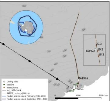
col-Figure 1. Map showing the location of the drilling sites of the S1C1 and TA192A firn cores (black points), the Dumont d’Urville and D17 stations (green points), the stake points (in brown; in-cluded the three closest stake points from the TA192A, namely the 18.3, 19.2, and 20.3 lines, and 156 km stake line), and the mean wind direction over the period 1957–2014 (in black). Isohypses (grey lines) shown in the main figure are simulations from adigi-tal elevation model, large-scale resolution. Radarsat Antarctic Map-ping Project Digital Elevation Model version 2 (Liu et al., 2001). The map of Antarctica on the top left displays the mean February and September sea ice extent over the period 1981–2010 extracted from the Nimbus-7 Scanning Multichannel Microwave Radiome-ter (SMMR) and Defense Meteorological Satellite Program Spe-cial Sensor Microwave/Imagers – SpeSpe-cial Sensor Microwave Im-age/Sounder (DMSP SSM/I-SSMIS) passive microwave data (http: //nsidc.org/data/nsidc-0051, last access: January 2018) (Cavalieri et al., 1996) (light blue and dark blue lines respectively), and the zoomed area (grey rectangle), while the grey rectangle in the mid-dle right zooms the area around the TA192A drilling site in order to show the three closest stake locations.
umn, for cations and anions respectively. Samples devoted to oxygen isotopic ratio were sent to LSCE (Gif-sur-Yvette, France) and analysed following two methods. First, δ18O was measured by the CO2/H2O equilibration method on a
Finni-gan MAT 252, using two standards calibrated to SMOW– SLAP international scales, with an accuracy of 0.05 ‰. Sec-ond, δ18O and δD were also measured using a laser cavity ring-down spectroscopy (CRDS) Picarro analyser, using the same standards, leading to an accuracy of 0.2 ‰ and 0.7 ‰ for δ18O and δD respectively. The resulting accuracy of d-excess, calculated using a quadratic approach, is 1.7 ‰.
2.2 Datasets
2.2.1 Instrumental data
To assess potential climate signals archived in our firn core records, we extracted meteorological data to ex-plore regional climate signals, and outputs of atmo-spheric models to explore synoptic scale climate sig-nals. The regional climate is well documented since 1957 thanks to the continuous meteorological monitor-ing at DDU station (https://donneespubliques.meteofrance. fr/?fond=produit&id_produit=90&id_rubrique=32, last ac-cess: January 2018), with one gap between March 1959 and January 1960. We extracted near-surface temperature, humidity, surface pressure, wind speed and wind direction data computed monthly and annual averages over the peri-ods 1957–2014 and 1998–2014.
The monthly average sea ice concentration was extracted from the Nimbus-7 Scanning Multichannel Microwave Ra-diometer (SMMR) and Defense Meteorological Satellite Program Special Sensor Microwave/Imagers – Special Sen-sor Microwave Image/Sounder (DMSP SSM/I-SSMIS) pas-sive microwave data (http://nsidc.org/data/nsidc-0051, last access: January 2018), over the 50–90◦S latitudinal range at a 25 km × 25 km grid resolution (Cavalieri et al., 1996). D’Urville summer sea ice extent was estimated by extract-ing the number of grid points coverextract-ing the area (50–90◦S, 135–145◦E) where the sea ice concentration is higher than 15 %, from December to January (included) for each year from 1998 to 2014.
SMB measurements from stake point data were obtained from the GLACIOCLIM observatory (https://glacioclim. osug.fr/, last access: January 2018). We extracted data from the three stakes closest to the TA drilling site, namely 18.3 (66.77◦S, 139.57◦E; 1.04 km from the TA drill site), 19.2 (66.77◦S, 139.56◦E; 83 m from the drilling TA site), and 20.3 (66.78◦S, 139.55◦E; 1.00 km from the drilling TA site), all spanning the period 2004–2014.
2.2.2 Database of surface snow isotopic composition
In order to compare the d-excess record from the TA firn core with available Antarctic values, we have up-dated the database of Masson-Delmotte et al. (2008), by adding 26 new data points from precipitation and firn core measurements provided with d-excess (Table 1). This in-cludes data from five ice cores from the database con-stituted by the Antarctica2k group (Stenni et al., 2017). Altogether, the updated database includes 777 locations. This includes 64 coastal sites at an elevation lower than 1000 m a.s.l., (with 19 new datasets). These data were extracted from our updated isotope database (Goursaud et al., 2018a) archived in the PANGAEA data library (https://doi.org/10.1594/PANGAEA.891279).
Table 1. Site, latitude (◦), longitude (◦E), and reference of new d-excess data added to Masson-Delmotte et al. (2008). Data in (a) correspond to precipitation, (b) data correspond to ice cores extracted from the Antarctica2k database (Stenni et al., 2017), and (c) data are new data compared to our prior database (Goursaud et al., 2017).
Site Latitude Longitude Reference
(a)
Frei (South Shetland Islands)* −62.20 301.04 Fernandoy et al. (2012) O’Higgins (north peninsula)* −63.32 302.10 Fernandoy et al. (2012)
Halley −75.58 333.50 Rozanski et al. (1993)
Base tte. Marsh −62.12 301.44 Rozanski et al. (1993) Rothera Point −67.57 291.87 Rozanski et al. (1993) Vernadsky −65.08 296.02 Rozanski et al. (1993)
Vostok −78.5 106.9 Landais et al. (2012)
DDU −66.7 140.00 Jean Jouzel, personal communication, June 2017 Neumayer −70.7 351.60 Schlosser et al. (2008)
Dome F −77.3 39.7 Fujita and Abe (2006)
Dome C −75.1 123.4 Schlosser et al. (2017)
(b)
EDC Dome C −75.10 123.39 Stenni et al. (2001)
NUS 08-7 −74.12 1.60 Steig et al. (2013)
NVFL-1 −77.11 95.07 Ekaykin et al. (2017)
WDC06A −79.46 247.91 Steig et al. (2013)
IND 25B5 coastal DML −71.34 11.59 Rahaman et al. (2016) (c)
OH-4* −63.36 302.20 Fernandoy et al. (2012)
OH-5* −63.38 302.38 Fernandoy et al. (2012)
OH-6* −63.45 302.24 Fernandoy et al. (2012)
OH-9* −63.45 302.24 Fernandoy et al. (2012)
OH-10* −63.45 302.24 Fernandoy et al. (2012)
KC −70.52 2.95 Vega et al. (2016)
KM −70.13 1.12 Vega et al. (2016)
BI −70.40 3.03 Vega et al. (2016)
GIP −80.10 159.30 Markle et al. (2012)
DE08-2 −66.72 112.81 Delmotte et al. (2000)
DSSA −66.77 112.81 Delmotte et al. (2000)
D15* −66.86 139.78 Jean Jouzel, personal communication, June 2017
TA192A −66.78 139.56 This study
Finally, data associated with “*” were not provided with a dating while data in italics have a sub-annual resolution. Note that DE08-2 and D15 ice cores were not dated.
2.2.3 Atmospheric reanalyses and back trajectories Unfortunately, because of the katabatic winds around DDU, no instrumental method allows reliable measurements of pre-cipitation (Grazioli et al., 2017a). We use outputs from ERA-Interim reanalyses (Dee et al., 2011b), which were shown to be relevant for Antarctic surface mass balance (Bromwich et al., 2011), to provide information on DDU intra-annual precipitation variability. We extracted these outputs from the grid point (0.75◦×0.75◦, ∼ 80 km × 80 km, point centered at 66.75◦S and 139.5◦E) closest to the TA drilling site over the period 1998–2014, at a 12 h resolution, and calculated daily, monthly, and annual average values. We also extracted 2 m temperature (2mT), 10 m u and v wind components (u10
and v10), and the geopotential height at 500 hPa (z500) over the whole Southern Hemisphere (50–90◦S), in order to
in-vestigate potential linear relationships between our records and the large-scale climate variability.
In order to identify the origin of air masses, back trajec-tories were computed using the HYSPLIT (Hybrid Single-Particle Lagrangian Integrated Trajectory) model. It is an at-mospheric transport and dispersion model developed by the National Oceanic and Atmospheric Administration (NOAA) Air Research Laboratory (Draxler and Hess, 1998), based on a mixing between Lagrangian and Eulerian approaches (Stein et al., 2015). We set the arrival point at the coordinates of the TA drilling site, at an initial height of 1500 m a.s.l., and used the NCEP/NCAR Global Reanalysis ARL archived
Figure 2. Representation of the sectors used to classify the last point of the simulated back trajectories by HYSPLIT over the pe-riod 1998–2014, defined as follows: (i) the eastern sector (0–66◦S, 0–180◦E), (ii) the plateau (66–90◦S, 0–180◦E), (iii) the Ross Sea sector (0–75◦S, 180–240◦E), and finally (iv) the western sector (0– 75◦S, 180–240◦E) and (50–90◦S, 240–360◦E).
data for forcing the meteorological conditions, as the ERA-Interim reanalyses are not available in the required extension. Earlier studies (e.g. Markle et al., 2012; Sinclair et al., 2010) highlighted good performances of NCEP outputs when com-pared with Antarctic station data after 1979. For instance, previous studies showed that the mean sea level pressure simulated at DDU and averaged on a 5-year running win-dow was well captured in NCEP reanalyses after 1986 (cor-relation coefficient > 0.8, bias < 4 hPa, and RMSE < 5 hPa) (Bromwich and Fogt, 2004; Bromwich et al., 2007). Also, Simmons et al. (2004) showed quasi-equal 12-month run-ning means of 2 m temperatures for the Southern Hemi-sphere between the European Re-Analyses ERA-40, the NCEP/NCAR, and the Climatic Research Unit CRUTEM2v products. We thus run daily 5-day back trajectories from Jan-uary 1998 to December 2014. Each back trajectory was anal-ysed for the geographical position of the last simulated point (the estimated start of the trajectory, 5 days prior to arrival at DDU) and classified into one of the following four regions, represented in Fig. 2 and defined by their longitude (long) and latitude (lat) as follows: (i) the eastern sector: (0–66◦S, 0–180◦E), (ii) the plateau: (66–90◦S, 0–180◦E), (iii) the Ross Sea sector: (0–75◦S, 180–240◦E), and finally (iv) the western sector: (0–75◦S, 180–240◦E) and (50–90◦S, 240– 360◦E).
2.2.4 Atmospheric general circulation and water stable isotope modelling: ECHAM5-wiso
The potential relationships between large-scale climate vari-ability and regional precipitation isotopic composition was also investigated through outputs of a nudged simulation performed with the atmospheric general circulation model ECHAM5-wiso (Roeckner et al., 2003), equipped with stable-water isotopes (Werner et al., 2011). We chose this model due to demonstrated skills to reproduce spatial and temporal patterns of water stable isotopes in Antarctica (Masson-Delmotte et al., 2008; Steen-Larsen et al., 2017; Werner et al., 2011; Goursaud et al., 2017) and in Greenland (Steen-Larsen et al., 2017).
In this study, we use the same simulation as Goursaud et al. (2017), in which the large-scale circulation (winds) and air temperature were nudged to outputs of the ERA-Interim reanalyses (Dee et al., 2011a). The skills of the model were assessed over Antarctica for the period 1979–2014. The model was run in a T106 resolution (i.e. ∼ 110 km × 110 km horizontal grid size). In the following, we used the subscripts ECH, TA, and S1C1 to differ ECHAM5-wiso outputs from the TA and S1C1 firn cores records respectively (e.g. δ18OTA
and δ18OECH). Note also that linear relationships are
consid-ered significant when the p value < 0.05. 2.2.5 Modes of variability
We tested the main modes of variability were imprinted in our recorded, especially
– the Southern Annual Mode (SAM) using the index defined by Marshall (2003) and archived on the National Center for Atmospheric Research website (Marshall, Gareth & National Center for Atmospheric Research Staff (Eds); last modified 19 March 2018; “The Climate Data Guide: Marshall Southern Annu-lar Mode (SAM) Index (Station-based)”; retrieved from https://climatedataguide.ucar.edu/climate-data/marshall-southern-annular-mode-sam-index, last access: January 2018).
– the El Niño–Southern Oscillation (ENSO) using the El Niño 3.4 index defined by the Climate Prediction Center of NOAA’s National Centers for Environ-mental Prediction and archived on their website (Trenberth, Kevin & National Center for Atmospheric Research Staff Eds); last modified 06 September 2018; “The Climate Data Guide: Nino SST Indices (Nino 1 + 2, 3, 3.4, 4; ONI and TNI)”; retrieved from https://climatedataguide.ucar.edu/climate-data/ nino-sst-indices-nino-12-3-34-4-oni-and-tni, last access: January 2018).
– the Interdecadal Pacific Oscillation (IPO), using the IPO Tripole Index (TPI) defined by Hen-ley et al. (2015) based on filtered HadISST and
ERSSTv3b sea surface temperature data and archived on the internet (https://www.esrl.noaa.gov/psd/data/ timeseries/IPOTPI, last access: 20 September 2018). – the Amundsen Sea Low pressure center (ASL) archived
one the National Center for Atmospheric Research web-site (Hosking, Scott & National Center for Atmospheric Research Staff Eds); last modified 19 March 2018; “The Climate Data Guide: Amundsen Sea Low in-dices”; retrieved from https://climatedataguide.ucar. edu/climate-data/amundsen-sea-low-indices, last ac-cess: January 2018).
3 Results
3.1 Firn core chronology 3.1.1 Ice core dating
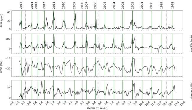
The firn core was dated using an annual layer counting method (Fig. 3). As in Goursaud et al. (2017), we used con-centrations in MSA and non-sea-salt (nss) SO2−4 (nssSO4).
We have explored the validity of an approach using a def-inition of nssSO4based on a sulfate-to-sodium mass ratio of
0.25 inferred from summer observations only. The multi-year study of size-segregated aerosol composition conducted at the coast of TA (the DDU station) has demonstrated that sea-salt aerosol is depleted in sulfate with respect to sodium in winter, with a sulfate-to-sodium mass ratio of 0.13 from May to October instead of 0.25 (i.e. the seawater composition) in summer (Jourdain and Legrand, 2002). Even at the high plateau station of Concordia, Legrand et al. (2017a) showed that sea-salt aerosol is depleted in sulfate in winter (sulfate-to-sodium ratio of 0.13 from May to October). We resampled the sulfate time series recorded in the TA with 12 points per year and inferred seasonal average values from averages over the corresponding subsets of points, as previously performed for isotopic records (Sect. 3.2). We then calculated nssSO4
(noted as nssSO∗4) using a sulfate-to-sodium ratio of 0.25 for points associated with months from November to February and 0.13 for points associated with months from March to September. Note that when ignoring the change in sulfate-to-sodium ratio in winter (i.e. applying a sulfate-sulfate-to-sodium ratio of 0.25 for all the points of the year), the mean nssSO4
value is lower by 18.2 %, decreasing from 36.5 ± 12.3 ppb to 43.1 ± 11.8 ppb for nssSO∗4(Fig. S1 in the Supplement). We thus applied a calculation of nssSO4for all points of our firn
core, only using the sulfate-to-sodium ratio obtained from summer observations, as [nssSO2−4 ] = [SO2−4 ] − 0.25 [Na+]. For depths lower than 10 m w.e., summer (December– January) peaks were identified (i) from nssSO4values higher
than 100 ppb, synchronous with MSA peaks (with no thresh-old), and (ii) for nssSO4values higher than 200 ppb (with or
without a simultaneous MSA peak). Double nssSO4 peaks
were counted as one summer (e.g. 2012, 2003, and 2001).
For depths higher than 10 m w.e., summer peaks were iden-tified for nssSO4 values higher than 27 ppb. The outcome
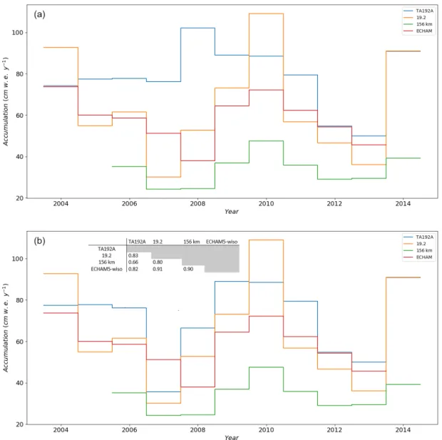
of layer counting allowed us to estimate annual layer thick-ness, which, combined with the density profile, allowed us to estimate annual SMB in the firn core. This estimated SMB was then compared with stake area data. The three stake data closest to the TA firn core (18.3, 19.2, and 20.3, not shown) depict the same inter-annual variability (pairwise coefficient correlations, r > 0.93 and p values, p < 0.05), giving con-fidence in the use of these measurements to characterize the inter-annual variability of local SMB. The comparison with the stake data shows that our initial layer-counted chronol-ogy results in a mismatch in the measured versus estimated SMB for the year 2008 (Fig. 4a). This mismatch can be re-solved by identifying one more summer peak in the chemical records (thin green line, Fig. 3). The revised firn core SMB record from this revised chronology shows correlation coef-ficients between the stake data and the TA firn core varying from 0.64 for 20.3 to 0.83 for 19.2 (p < 0.05), with coherent inter-annual variability (Fig. 4b).
Peaks in δ18OTAor d-excessTAwere not used in our layer
counting, so that our age scale is independent of a climatic interpretation of water stable isotopes (e.g. assumption of synchronicity between temperature seasonal cycles and wa-ter stable isotope records). We note an uncertainty in layer counting of 3 years when comparing the outcome of layer counting using chemical records with δ18OTA peaks, which
have nonetheless been excluded from our dating, as they do not improve the correlations, either between the recon-structed SMB and the stake data or between our records and the ECHAM5-wiso simulations (Tables S1 to S3).
As a result, we consider the “best guess” chronology re-sults from the annual layer counting based on nssSO4 and
MSA refined with the comparison with stake data, giving a total of 18 summer peaks (green vertical lines, Fig. 3). In the following, we thus use the dated firn core records covering the complete period 1998–2014. We note that our chronol-ogy is more robust for the period 2004–2014, for which stake area SMB data are available.
3.1.2 Potential post-deposition effects
In order to test whether the available d-excessTArecords are
not affected by post-deposition effects, one may apply cal-culations of diffusion (e.g. Jones et al., 2017; Johnsen et al., 2000; van der Wel et al., 2015). However, many records are not available as depth profiles, and annual accumulation rate data are missing, precluding a systematic approach. We thus applied a simple approach to quantify how the seasonal δ18OTAand d-excessTAamplitudes vary through time in firn
records, as an indicator of potential post-diffusion effects. For this purpose, we calculate the ratio between the mean amplitude of the most recent three complete seasonal cycles (2011–2014 for TA) and the average seasonal amplitude for the whole record (1998–2014 for TA). If seasonal cycles are
Figure 3. Identification of annual layers in the TA192A ice core based on the dual identification of nssSO2−4 and MSA summer peaks and comparison of estimated accumulation with annual accumulation measured at the closest stakes (not shown). The thick vertical green lines correspond to summer peaks identified from chemical signals, while the thin vertical green line shows the additional identification of summer 2008 added to the counted summers from the comparison between the estimated accumulation and the accumulation record from the closest stake data (see Fig. 3). Vertical dashed lines highlight equivocal summer peaks with a sometimes small signal in only one of the chemical records. Water stable isotope records were not used to build the timescale. Note that double peaks in both δ18O and d-excess occur repeatedly within one counted year.
stable through time, and if there is no significant smooth-ing due to post-deposition effects, we should obtain a ratio of 1. However, it is expected to be above 1 in the case of large post-deposition smoothing. We obtain a ratio of 0.5 for δ18OTA data, possibly reflecting the inter-annual variability
of the δ18O seasonal amplitude. We repeated the same ex-ercise with all eight other sub-annual δ18O records from our database (Table S4). Discarding an outlier (NUS 08-7), all ra-tios are between 1.0 and 2.9. Rara-tios based on d-excess ampli-tudes are similar to those found for δ18O (Table S5). For the TA firn core, we again obtain a ratio of 1.1 for d-excessTA.
We also note high ratios for d-excess data in the NUS 08-7. Except for the ratios calculated in the WDC06A, which no-tably differs for d-excess (1.1) compared to δ18O (2.9), other ratios for d-excess data vary between 1.0 and 1.4, with 20 % maximum difference compared to the corresponding ratio for δ18O data.
For the TA, we also estimated the diffusion length (Küt-tel et al., 2012) and found mean diffusion lengths of 1.4 ± 0.3 months for δ18OTA (with a maximum of 1.9 months in
2007) and 1.6±0.5 months for d-excessTA(with a maximum
of 2.4 months in 2007).
These results suggest that potential post-deposition effects in the TA can be neglected. Notwithstanding, a potential loss of seasonal amplitude in the other average time series
com-pared to the most recent seasonal cycles cannot be discarded and has to be considered in the comparison of seasonal am-plitudes, from one core to the other, in the comparison with the seasonal amplitude of precipitation δ18O time series, and with ECHAM5-wiso outputs.
3.2 Mean values
3.2.1 Mean climate from instrumental data
Before reporting the mean values from TA records, we de-scribe the available meteorological data. A time-averaged statistical description of the available meteorological data measured at DDU, the station closest to the drilling site, is given in Table 2 for the whole available measurement pe-riod prior to 2015 (1957–2014) and over the pepe-riod cov-ered by our TA records, 1998–2014. For all the considcov-ered parameters (near-surface temperature, wind direction, wind speed, humidity, and surface pressure), the time-averaged values differ by less than 8 % (the maximum deviation be-ing for the wind direction) over the period 1998–2014 com-pared to the whole available period. Standard deviations cal-culated over these two time periods also differ by less than one respective standard deviation unit, except for wind di-rection, which shows much less variability over the recent period. We conclude that the local climate of the period
Figure 4. Annual accumulation (cm w.e. yr−1)estimated from the layer counting in the TA192A firn core (blue line), measured at the closest stake point 19.2 (orange line), from the 156 km network stake data (green line) and extracted from the ECHAM5-wiso model (red line), before (a) and after (b) adding the identification of summer 2008 in a time interval of low accumulation rates and skipped in the initial layer-counting approach due to the lack of a signal in the MSA record (thin green line in Fig. 2). Correlations between time series (TA192A series inferred from the second dating) are inserted in the lower plot, with all linear relationships being significant (p < 0.05).
1998–2014 is representative of the multi-decadal climate state since 1957. In ERA-Interim, the average precipitation is 46.0 ± 26.9 cm w.e. yr−1over the period 1998–2014.
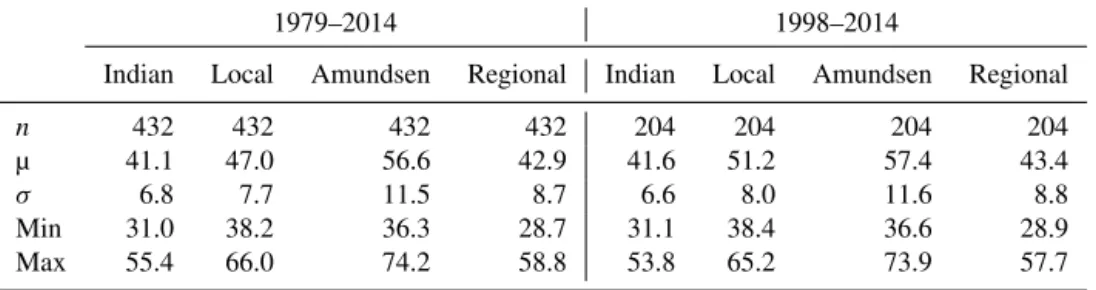
Finally, we compare the statistical description of the sea ice concentration for the four aforementioned regions (Sect. 2.2) over the available period 1979–2014, with the pe-riod covered by the TA firn core 1998–2014 (Table 3). We note that the mean difference between the two periods is maximum for the local sea ice concentration (135–145◦E),
with 8.9 % difference, whereas it remains below 1.5 % for the other sectors. The extrema (minimum and maximum val-ues) vary by 0.5 % on average (all regions included) from one sector to another, with a maximum difference of 2.9 %. As a result, the mean sea ice concentrations of the period 1998–
2014 are also representative for the last decades over large sectors from the Amundsen Sea to Indian Ocean.
3.2.2 Mean values recorded in the TA firn core
Time-averaged values calculated from TA records are reported in Table 4. The average SMBTA is 75.2 ±
15.0 cm w.e. yr−1. Stake data points from GLACIOCLIM show that this site of high accumulation is located in an area of large spatial variability. This feature is confirmed by the values given by (i) the stake data closest to the TA site (19.2, 100 m for the TA site and associated with a 76.6 ± 25.8 cm w.e. yr−1mean accumulation rate) compared to fur-ther stake data (18.2, 1.04 km from the TA site and
associ-Table 2. Number of points (n), time averages (µ), standard deviation (σ ), minimum (min), and maximum (max) values of all the monthly meteorological observations at Dumont d’Urville from Météo France over the period 1957–2014 (with a gap between March 1959 and January 1960, inclusive) and over the period 1998–2014 for near-surface temperature (Ts,◦C), wind speed (ws, m s−1), wind direction
(wd,◦E), relative humidity (RH, %), and annual precipitation and accumulation (precipitation minus evaporation and sublimation) from ERA-Interim reanalyses (Prec. ERA, mm w.e. yr−1).
1957–2014 Ts ws wd RH Ts ws wd RH Prec. ERA (◦C) (m s−1) (◦E) (%) (◦C) (m s−1) (◦E) (%) (cm w.e. yr−1) n 730 719 383 717 202 201 201 199 µ −10.9 9.6 145.3 61.4 −11.1 9.1 133.8 60 46.0 σ 6 2.1 22.4 7.6 6.0 1.8 15.8 8.3 26.9 Min −23.5 4.9 90 34 −22.1 4.8 1.5 34.0 1.5 Max 1 19.5 220 86 0.9 14.1 172.4 85.5 147.8
Table 3. Number of points (n), time averages (µ), standard deviation (σ ), minimum (min), and maximum (max) values of monthly meteoro-logical sea ice concentration over the periods 1979–2014 and 1998–2014 extracted from the Nimbus-7 Scanning Multichannel Microwave Radiometer (SMMR) and Defense Meteorological Satellite Program Special Sensor Microwave/Imagers – Special Sensor Microwave Im-age/Sounder (DMSP SSM/I-SSMIS) passive microwave data (http://nsidc.org/data/nsidc-0051, last access: January 2018) (Cavalieri et al., 1996), and for the four regions defined as (i) “local” (135–145◦E), (ii) “Indian” (100–145◦E), (iii) “Amundsen” (160–205◦E), and (iv) “re-gional” (100–205◦E).
1979–2014 1998–2014
Indian Local Amundsen Regional Indian Local Amundsen Regional
n 432 432 432 432 204 204 204 204
µ 41.1 47.0 56.6 42.9 41.6 51.2 57.4 43.4
σ 6.8 7.7 11.5 8.7 6.6 8.0 11.6 8.8
Min 31.0 38.2 36.3 28.7 31.1 38.4 36.6 28.9
Max 55.4 66.0 74.2 58.8 53.8 65.2 73.9 57.7
ated with a 47.7±15.7 cm w.e. yr−1mean accumulation rate), (ii) our mean SMB reconstruction from the S1C1 ice core al-most 4 times lower than for the TA (21.8 ± 6.9 cm w.e. yr−1; Goursaud et al., 2017), and (iii) mesoscale fingerprints such as the SMB estimated for coastal Adélie Land by Pettré et al. (1986), based on measurements at stakes located from 500 m to 5 km from the coast (Table 2).
The average δ18OTA value is −19.3 ‰ ± 3.1 ‰, close
to the average δ18OS1C1 of −18.9 ‰ ± 1.7 ‰, and the
av-erage d-excessTA is 5.4 ‰ ± 2.2 ‰. Compared to the 64
points located at an elevation lower than 1000 m a.s.l. from our database, the δ18OTA and d-excessTA average values
are slightly higher than the average low-elevation records (−22.7 ‰ ± 8.8 ‰ and 4.8 ‰ ± 2.3 ‰ for δ18O and d-excess respectively, Fig. 5). Finally, the average TA concentrations in Na+, MSA, and nssSO4are 126.0 ± 276.5, 4.5 ± 5.6, and
36.5 ± 44.2 ppb respectively. Note that the Na+average con-centration value is affected by strong peaks in 2003 and 2004 with annual values of 369.4 and 388.5 ppb. Excluding these two peaks, the average Na+concentration is reduced to 93.2 ppb (with a standard deviation of 38.6 ppb). These con-centrations will be discussed later in Sect. 4.4.
To summarize our findings, the TA records encompass a period (1998–2014) representative of multi-decadal mean climatic conditions. The isotopic mean values appear lower than the average of other Antarctic low-elevation records (as shown in Fig. 4). The local SMB is remarkably high for East Antarctica, consistent with stake measurements performed close to the TA site.
3.3 Inter-annual variations
In the following, we refer to seasons as follows: summer (De-cember to February), autumn (March to May), winter (June to September), and spring (October and November). This cutting was defined based on the mean seasonal cycle of temperature, showing the highest values from December to February, and a plateau of low values from May to Septem-ber (Fig. 8a). In the TA records, resampled with 12 points per year, we identified seasonal average values by calculat-ing averages over the correspondcalculat-ing subsets of points (e.g. for autumn, we select from the third to the fifth points out of the 12 resampled points within the year). We are fully aware that this is a simplistic approach, assuming a regular distri-bution of precipitation year round, and that our chronology is
Table 4. Time averages (µ) and standard deviation (σ ) of the reconstructed accumulation (cm w.e.) and of the signals recorded in the TA192A ice core obtained from the resampling of the isotopic and chemical variables for δ18O (‰), d-excess (‰), Na, MSA, and nssSO4(ppb), over
the 17 annual values.
Accumulation δ18O d-excess Na+ MSA nssSO4
(cm w.e.) (‰) (‰) (ppb) (ppb) (ppb)
µ 75.2 −19.3 5.4 126.0 4.5 36.5
σ 15.0 3.1 2.2 276.5 5.6 44.2
Figure 5. Spatial distribution of δ18O (a, ‰) and d-excess (b, ‰) in surface Antarctic snow based on our updated database combining data from precipitation, surface snow, pits, and shallow ice cores. Bigger points with a black edge correspond to new data compared to Masson-Delmotte et al. (2008).
more accurate for summer than for other seasons, due to the layer-counting method. We nevertheless checked that the dis-tribution of precipitation simulated by ERA-Interim within each year is rather homogeneous (Table S6).
3.3.1 Trends in time series
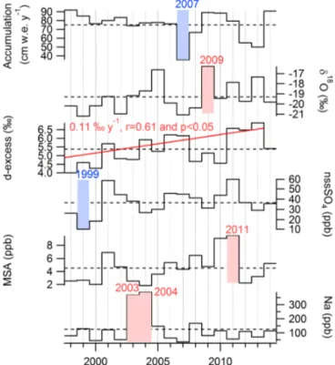
Here we report the analysis of potential trends from 1998 to 2014 and the identification of remarkable years. Figures 6 and 7 display the time series of meteorological variables, Du-mont d’Urville summer sea ice extent and TA records over 1998–2014. In Figs. 6 and 7, we chose not to display stan-dard deviations for readability, but they are reported in the Supplement (Figs. S2 and S3).
Significant increasing trends are detected in the annual values of d-excessTA(0.11 ‰ yr−1, r = 0.61 and p < 0.05)
as well as of Dumont d’Urville summer sea ice extent (r = 0.77, p < 0.05).
3.3.2 Pairwise linear regressions between variables We performed pairwise linear regressions for all records (me-teorological and firn core records), using, on the one side,
annual averages and, on the other side, monthly or seasonal values. As previously observed by Comiso et al. (2017), we report a significant anti-correlation between annual regional sea ice concentration (i.e. 100–205◦E, but not with other sectors) and DDU near-surface air temperature (r = −0.56 and p < 0.05). This relationship is strongest in autumn (r = −0.75 and p < 0.05), where it holds for sea ice in all sectors, and disappears in spring or summer. Confirming earlier stud-ies (Minikin et al., 1998), we observe a close correlation be-tween annual concentrations of MSA and nssSO4(r = 0.76,
p <0.05). Statistically significant linear relationships ap-pear between the isotopic signals (δ18OTA and d-excessTA)
and nssSO4 in spring (r = 0.65 and r = 0.55 for δ18OTA
and d-excessTArespectively, p < 0.05) and only between
d-excessTA and nssSO4 in autumn (r = 0.65 and p < 0.05).
We find no relationship between δ18OTAand the DDU
near-surface temperature. Our record depicts a significant anti-correlation between annual values of SMBTAand d-excessTA
(r = −0.59 and p < 0.05), as well as a significant correla-tion between d-excessTAand Dumont d’Urville summer sea
ice extent (r = 0.65 and p < 0.05). Finally, a systematic pos-itive significant correlation is identified between d-excessTA
Figure 6. Meteorological time series over the period 1998–2014 av-eraged at the inter-annual scale. Near-surface temperature (◦C), rel-ative humidity (%), sea level pressure (hPa), wind speed (m s−1), and direction (◦E) were provided by Météo France. The local sea ice concentration (%) is extracted in the 135–145◦E sector (with a latitudinal range of 50–90◦S) from the Nimbus-7 Scanning Multi-channel Microwave Radiometer (SMMR) and Defense Meteorolog-ical Satellite Program Special Sensor Microwave/Imagers – Special Sensor Microwave Image/Sounder (DMSP SSM/I-SSMIS) passive microwave data (Cavalieri et al., 1996). Horizontal dashed lines cor-respond to the climatological averages over 1998–2014 for each pa-rameter. Remarkable years, i.e. associated with values deviating by at least 2 standard deviations from the climatological mean value, are highlighted with red shading (positive anomalies) or blue shad-ing (negative anomalies). The same figure with standard deviations is available in the Supplement (Fig. S2).
and δ18OTA, except in summer. It is the strongest in austral
spring, with a correlation coefficient of 0.75 (with a slope of 0.61 ‰ ‰−1).
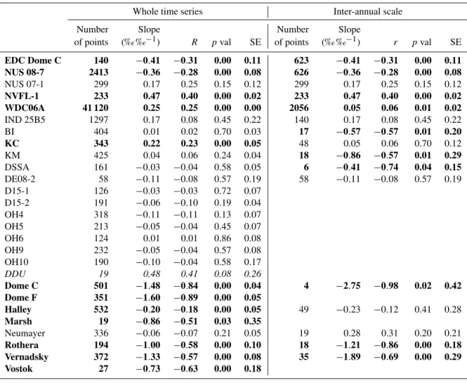
In order to understand the specificities of the TA record, we explored the temporal correlation between δ18O and d-excess from all available Antarctic records (Table 5, cells in bold for significant relationships), using all data points (in order to be able to exploit non-dated depth profiles) as well as inter-annual variations, when available. When focusing on significant results, we note that most precipitation datasets depict an anti-correlation between d-excess and δ18O (three out of nine precipitation records). Although we are cautious with the short DDU precipitation time series (with only 19 points, and p values = 0.08, cell in italics in Table 5), it
Figure 7. Dated TA192A ice core annually averaged records over the period 1998–2014: accumulation, cm w.e. yr−1; concentrations of Na+ (ppb), nssSO4(ppb), MSA (ppb), δ18O (‰), and d-excess
(‰). Horizontal dashed lines correspond to 1998–2014 average val-ues. Remarkable years (i.e. associated with values deviating by at least 2 standard deviations from the climatological mean value) are highlighted with red shading (positive anomalies) or blue shading (negative anomalies). The same figure with standard deviations is available in the Supplement (Fig. S3).
shows a positive relationship, similar to the one identified in the TA record. We conclude that the positive correlation observed in the TA records is specific to the coastal Adélie Land region, which is unusual in an Antarctic context. 3.3.3 Remarkable years
Using only annual SMB, water stable isotope, and chemistry TA records, we finally searched for remarkable years, defined here as deviating from the 1998–2014 mean value by at least 2 standard deviations. We highlight three remarkable years (red-shaded for high values and blue-shaded for low values, Figs. 6 and 7):
– 2007, with very low SMBTA;
– 2009, with remarkably high δ18OTA;
– 2011, with high MSA, Dumont d’Urville summer sea ice extent, and wind speed values.
We had previously noted that the years 2003 and 2004 are associated with very high Na+ values and add that the year 1999 experienced low nssSO4values.
Table 5. The d-excess versus δ18O linear relationship of data from our database provided with d-excess over the whole time series (left side of the table) and over annual averages (inter-annual scale, right side of the table): slope (‰ ‰−1), correlation coefficient (r), p value (p val), and standard error of the slope (SE, ‰ ‰−1). Cells in bold show a significant relationship (p < 0.05) and the cell in italic is to be taken with caution (see DDU line, p < 0.10). Inter-annual relationships could not be computed for undated data (D15 and OH ice cores) or for precipitation data monitored for too short of a time and thus appear as empty cells.
Whole time series Inter-annual scale
Number Slope Number Slope
of points (‰ ‰−1) R pval SE of points (‰ ‰−1) r pval SE EDC Dome C 140 −0.41 −0.31 0.00 0.11 623 −0.41 −0.31 0.00 0.11 NUS 08-7 2413 −0.36 −0.28 0.00 0.08 626 −0.36 −0.28 0.00 0.08 NUS 07-1 299 0.17 0.25 0.15 0.12 299 0.17 0.25 0.15 0.12 NVFL-1 233 0.47 0.40 0.00 0.02 233 0.47 0.40 0.00 0.02 WDC06A 41 120 0.25 0.25 0.00 0.00 2056 0.05 0.06 0.01 0.02 IND 25B5 1297 0.17 0.08 0.45 0.22 140 0.17 0.08 0.45 0.22 BI 404 0.01 0.02 0.70 0.03 17 −0.57 −0.57 0.01 0.20 KC 343 0.22 0.23 0.00 0.05 48 0.05 0.06 0.70 0.12 KM 425 0.04 0.06 0.24 0.04 18 −0.86 −0.57 0.01 0.29 DSSA 161 −0.03 −0.04 0.58 0.05 6 −0.41 −0.74 0.04 0.15 DE08-2 58 −0.11 −0.08 0.57 0.19 58 −0.11 −0.08 0.57 0.19 D15-1 126 −0.03 −0.03 0.72 0.07 D15-2 191 −0.06 −0.10 0.19 0.04 OH4 318 −0.11 −0.11 0.13 0.07 OH5 213 −0.05 −0.04 0.45 0.07 OH6 124 0.01 0.01 0.86 0.08 OH9 232 −0.05 −0.04 0.57 0.08 OH10 190 −0.10 −0.04 0.58 0.17 DDU 19 0.48 0.41 0.08 0.26 Dome C 501 −1.48 −0.84 0.00 0.04 4 −2.75 −0.98 0.02 0.42 Dome F 351 −1.60 −0.89 0.00 0.05 Halley 532 −0.20 −0.18 0.00 0.05 49 −0.23 −0.12 0.41 0.28 Marsh 19 −0.86 −0.51 0.03 0.35 Neumayer 336 −0.06 −0.07 0.21 0.05 19 0.28 0.31 0.20 0.21 Rothera 194 −1.00 −0.58 0.00 0.10 18 −1.21 −0.86 0.00 0.18 Vernadsky 372 −1.33 −0.57 0.00 0.08 35 −1.89 −0.69 0.00 0.29 Vostok 27 −0.73 −0.63 0.00 0.18
In summary, we identify increasing trends in d-excessTA
and sea ice concentration, no significant correlation between δ18OTA and DDU near-surface temperature, and an
anti-correlation between d-excessTA and SMBTA. We also note
two remarkable years in SMBTA (dry 2007) and δ18OTA
(high 2009). Finally, no systematic relationships are iden-tified between chemistry and water stable isotope signals (e.g. parallel trends, inter-annual correlation, and remark-able years).
3.4 Intra-annual scale
3.4.1 Mean cycles
The high resolution of the TA record allows us to describe the mean seasonal cycles (Fig. 8), as well as to explore the inter-annual variability of the seasonal cycle.
Among the meteorological variables, only near-surface temperature, relative humidity, and sea level pressure show a clear seasonal cycle. Temperature (Fig. 8a) is minimum in July and maximum in January, while relative humidity and pressure (Fig. 8b and c respectively) are minimum in spring (in November and October respectively) and maxi-mum in winter (in August and June respectively), as reported in earlier studies (Pettré and Périard, 1996). The average sea-sonal cycles of wind speed and wind direction are flat but marked by large inter-annual variations (Fig. 8d and e). Fi-nally, the local sea ice concentration shows a rapid advance from March to June, a plateauing from June to October, and a rapid retreat from October to November, with a minimum in February (Fig. 8c), as previously reported by Massom et al. (2013).
In the TA firn core, Na, nssSO4, and MSA show
sym-metric cycles with minima in winter and maxima in sum-mer (by construction of our timescale) (Fig. 8g–i), consistent
Figure 8. Mean seasonal cycles over the period 1998–2014. Meteorological observations are averaged from daily data, for near-surface temperature (a,◦C), relative humidity (b, i %), surface pressure (c, hPa), wind speed (d, m s−1), wind direction (e,◦E), and local sea ice concentration, i.e. averaged over a 135–145◦E ridge (f, %). Seasonal cycles from ice core records are averaged from the resampled time series for Na (g, ppb), nssSO4(h, ppb), MSA (i, ppb), δ18O (j, ‰), and d-excess (k, ‰). The inter-annual standard deviation is highlighted
with the grey shading.
with previous studies of aerosols and ice core signals (e.g. Preunkert et al., 2008). The δ18OTA seasonal cycle is
sur-prisingly asymmetric (Fig. 8j), with a maximum in Decem-ber and a minimum in April, thus not in phase with the sea-sonal cycles of local sea ice concentration (Fig. 8f) or DDU
temperature (Fig. 8a). The mean d-excessTAseasonal cycle
(Fig. 8k) is marked by a maximum in February, 2 months after the δ18OTA maximum, and a minimum in October, 6
months after the δ18OTA minimum. We then calculated the
the amplitude of the mean seasonal cycle, due to the dif-ferent timing of peaks from one year to another. The mean δ18OTA seasonal amplitude is 8.6 ‰ ± 2.1 ‰, more than 3
times higher than found in the S1C1 ice core, and close to the DSSA mean δ18O seasonal cycle of 8.0 ‰ ± 2.8 ‰. The mean d-excessTAseasonal amplitude is 6.5 ‰ ± 2.8 ‰, close
to the DSSA value of 5.3 ‰ ± 1.0 ‰. Compared with other precipitation and firn/ice core isotopic data from other re-gions of Antarctica (Table S7), the average seasonal ampli-tude obtained from TA δ18O is closest to the one obtained at KM, BI sites in Dronning Maud Land, and Vernadsky or Rothera on the peninsula but is much larger than identified from NUS 08-7 or WDC06A and significantly smaller than at Halley (by a factor of almost 2), Neumayer (a factor of 2.3), Dome C, or Dome F (a factor of ∼ 4). In addition to DSSA, the average seasonal amplitude obtained from TA d-excess is also comparable to the one obtained in the KM, BI, and IND25B5 firn cores in Dronning Maud Land but is systematically higher (by a factor higher than 3) than in pre-cipitation datasets. This calls for systematic comparisons of d-excess seasonal amplitudes in precipitation and snow data. Due to their common symmetric aspect, significant posi-tive linear relationships emerge from the mean seasonal cy-cles of (i) temperature, nssSO4, and MSA (r > 0.93 and
p <0.05), (ii) nssSO4 and MSA (r = 0.97 and p < 0.05),
(iii) nssSO4 and Na+ (r = 0.93 and p < 0.05), and finally
(iv) δ18O with nssSO4(r = 0.75 and p < 0.05). Due to the
asymmetry of water stable isotope seasonal cycles, no linear relationship is detected between the seasonal cycles of DDU near-surface temperature, δ18OTA, and d-excessTA. Finally,
the seasonal cycle of d-excessTA is clearly anti-correlated
with all sea ice concentration indices (local, Indian, Amund-sen, and regional), with correlation coefficients varying be-tween −0.83 and −0.80.
3.4.2 Inter-annual variability of peaks
Over the whole period covered by the TA firn core (1998– 2014), the seasonal cycle of δ18OTA shows a large
inter-annual variability (Table 6). δ18OTAmaximum values occur
primarily in summer (41 % of the time) and winter (41 %) and more rarely in spring (12 %) and in autumn (6 %). The same feature is observable for d-excessTA, which most of the
time has its maximum in summer (38 %) and winter (43 %) and more scarcely in spring (6 %) and in autumn (13 %).
In summary, the TA water stable isotope seasonal cycles display an asymmetry, with higher isotopic values in austral spring than in austral autumn. The d-excessTAseasonal cycle
is anti-correlated with the reconstructed SMB. Finally, the TA isotopic seasonal cycles show a high inter-annual vari-ability from one seasonal cycle to another one, with no re-current pattern between those of δ18OTAand d-excessTA.
Table 6. Fraction of annual maxima (%) of δ18O and d-excess iden-tified during each season: austral summer (DJF, i.e. from December to February), austral autumn (MAM, i.e. from March to May), aus-tral winter (JJAS, i.e. from June to September), and ausaus-tral spring (ON, i.e. from October to November) in the data over the period 1998–2014 and in the ECHAM5-wiso simulation (model) over the period 1998–2013. The analysis is based on resampled data (ice core) and monthly values (model).
Variable Source Period DJF MAM JJAS ON δ18O Data 1998–2014 41 6 41 12 Model 1998–2013 63 0 12 25 d-excess Data 1998–2014 41 12 41 6 Model 1998–2013 0 69 31 0
3.5 Influence of synoptic weather on TA records: insights from ECHAM5-wiso simulation, ERA-Interim reanalyses, back trajectories, and modes of variability
In order to explore the influence of the synoptic-scale weather on TA records, we explore outputs of ECHAM5-wiso and back-trajectory calculations, driven by atmospheric reanalyses. None of the associated atmospheric simulations resolve local processes such as katabatic winds or sea breeze. We used the ECHAM5-wiso model outputs to explore the following questions: (i) do ECHAM5-wiso outputs show similarities with the corresponding observed variables for their inter-annual variability, trends, and remarkable years? (ii) What are the simulated seasonal cycles for δ18O and d-excess? (iii) What are the simulated relationships between lo-cal near-surface air temperature and δ18O and between δ18O and d-excess at the seasonal and inter-annual scales? (iv) Are there significant relationships between our isotopic records and the large-scale climatic variability?
3.6 ECHAM5-wiso similarities with the corresponding observed variables
For inter-annual variations, the annual means of DDU near-surface temperature and the simulated 2 m temperature (2mTECH) are significantly correlated (slope of 0.50 ± 0.14,
r =0.67, and p < 0.05). This relationship is valid for all sea-sons. It is the strongest in winter (slope of 1.1 ± 0.1◦C◦C−1, r =0.93 and p < 0.05) and the weakest in summer (slope of 0.98 ± 0.3◦C◦C−1, r = 0.69, and p < 0.05). There is no
significant correlation between water stable isotope records from the TA and simulated by the ECHAM5-wiso, for either δ18O or d-excess. Finally, we found no significant trend in any model output over 1998–2014.
In terms of remarkable years, ECHAM5-wiso shows a low δ18OECHmean value in 1998 and a high d-excessECHmean
value in 2007 (Fig. S4). Only the year 2007 is remarkable in both the data (low reconstructed SMB) and the model.
We thus explored the model more deeply. The highest d-excess value was simulated 7 May (Table S8). When com-paring from 6 to 8 May 2007, with daily averages over the period 1979–2014, the model simulates similar near-surface temperature but particularly low precipitation and wind com-ponents (zonal and meridional). Despite the small precipita-tion amount, the daily isotopic anomaly is sufficiently large to drive the annual anomaly (Fig. S5). The d-excess values higher than 30 ‰ (threshold chosen as it corresponds to the maximum d-excess mean + standard deviation simulated by ECHAM5-wiso over Antarctica at the monthly scale; see Fig. S6) occur only four other times over 1998–2014. We nevertheless remain cautious with these values, which could be due to a numerical artefact.
t2mECH–δ18OECH, SMBECH–d-excessECH, and δ18OECH–
d-excessECH relationships are not identified in
ECHAM5-wiso seasonal or annual outputs. Likewise, no significant re-lationship could be identified between d-excessTAand SMB
simulated by ERA using both annual and seasonal values. 3.6.1 Simulated seasonal cycles for δ18O and d-excess We now explore the seasonal variations in δ18OECH and
d-excessECH over the period of simulation (1998–2014,
Ta-ble 6). The peaks in t δ18OECHpredominantly occur in spring
and summer (25 % and 63 % respectively), while they only happen 12 % of the time in winter and never in autumn. The d-excessECHpeaks most often in autumn (69 %) and
secon-darily in winter (31 %), but never during the other seasons. As a result, the model simulates more regular isotopic sea-sonal cycles with δ18O maxima during spring to summer sea-sons and d-excess maxima during autumn to winter seasea-sons, than identified in the TA record.
3.6.2 Relationships with the large-scale climatic variability
The ERA-Interim outputs allow us to investigate whether the large-scale climatic variability influences the isotopic com-position of Adélie Land precipitation recorded in the TA firn core. We looked at the simulated linear relationships between the TA isotopic records (δ18OTA and d-excessTA)
with the ERA-Interim outputs (2mT, u10, v10, and z500, Sect. 2.2). Here we report only significant relationships with absolute correlation coefficients higher than 0.6. For δ18OTA,
we found a correlation with 2mT over the Antarctic plateau (Fig. 12a), as well as a correlation with v10 (Fig. 12b) along the westerly wind belt, at ∼ 55◦S, 100◦E and ∼ 55◦S,
130◦E in the Indian Ocean and at ∼ 55◦S, 10–50◦E in the Atlantic Ocean, and a very little area on coastal Dron-ning Maud Land at ∼ 60◦S, 30–40◦E. For d-excessTA, we
found a correlation with 2mT (Fig. 12c) toward the Lam-bert Glacier at ∼ 70–80◦S, 30–40◦E and an anti-correlation in the south of the peninsula at ∼ 55–65◦S, 250–300◦E. Fi-nally, we noted a correlation between d-excessTA and u10
(Fig. 12d) at a very narrow area of Dronning Maud Land at ∼ 80◦S, 10–20◦E and an anti-correlation on the westerly
wind belt in the Atlantic Ocean at ∼ 55◦S, 40–50◦E. No
cor-relation is found with z500, δ18OTA, or d-excessTA.
Note that no significant relationship is obtained between the TA records and any mode of variability.
3.6.3 Origin of air masses
Finally, we used the HYSPLIT back-trajectory model to count the proportion (percentage) of air mass back trajec-tories, based on daily calculations over the period 1998– 2014, and averaged at the annual and seasonal scale, from four different regions (Sect. 2.3): the plateau, the eastern At-lantic Ocean and the Indian Ocean (eastern sector), the Ross Sea sector (RSS), and the West Antarctic Ice Sheet with the Pacific Ocean and the western Atlantic Ocean (western sector), as displayed in Fig. 2. On average, the highest an-nual proportion of air masses comes from the eastern sector (54.1 ± 8.3 %) and the East Antarctic plateau (32.5 ± 4.9), while a small proportion of air masses come from the west-ern sector (9.7 ± 3.7 %) and from the RSS (3.6 ± 1.3 %). A k-mean clustering over the last points of the whole back trajectories indicate two main origins, in the Indian Ocean (62.4◦S, 131.7◦E) and in the coastal West Antarctic Ice Sheet (73.4◦S, 227.5◦E).
Inter-annual variations in back trajectories (Fig. 9b) reveal a positive trend for the fraction of air masses coming from the western sector (slope of 0.41 ± 0.16 % yr−1, r = 0.55, and p < 0.05) and remarkable years: 1999, which was identi-fied as having a remarkable high δ18O value and low nssSO4
value in our TA records, is here associated with a minimum of back trajectories from the plateau, and the year 2011, which was associated with particularly high MSA in our TA record, shows a particularly low proportion of air masses coming from the eastern sector and a particularly high pro-portion of air masses coming from the Ross and western sec-tors.
The seasonal cycles of back trajectories per region are shown in Fig. 9c. The percentage of back trajectories coming from the plateau displays peaks in autumn and spring (March and November), those from the Ross Sea sector in winter and summer (January and June), those from the eastern sector in autumn and winter (May and August), and finally those from the western sector in spring (November). We note a signifi-cant linear correlation between the seasonal cycles of the per-centage of δ18O and back trajectories coming from the Ross Sea sector (r = 0.68 and p < 0.05) and from the western sec-tor (r = 0.59 and p < 0.05) and between the seasonal cycles of d-excess and the percentage of back trajectories coming from the western sector (r = −0.67 and p < 0.05).
Finally, we associated each daily back trajectory with daily precipitation δ18O and d-excess values simulated by ECHAM5-wiso in the precipitation and classified the time series for each variable by back-trajectory sectors. We then
Figure 9. Results of daily back-trajectory calculations over the period 1998–2014 with (i) the percentage (%) of the sum of back trajectories passing over each defined region: (i) the eastern sector (0–66◦S, 0–180◦E), (ii) the plateau (66–90◦S, 0–180◦E), (iii) the Ross Sea sector (0–75◦S, 180–240◦E), and finally (iv) the western sector (0–75◦S, 180–240◦E) and (50–90◦S, 240–360◦E) (see Sect. 2.3), and with (ii) averages at the annual scale (b) and at the mean seasonal scale (c). In (b) and (c)) horizontal dashed lines correspond to the mean value and vertical solid lines to standard deviations. Remarkable years, i.e. associated with values deviating by at least 2 standard deviations from the climatological mean value, are highlighted with red shading (positive anomalies) or blue shading (negative anomalies).
computed the corresponding seasonal cycles (Fig. 10). The mean δ18OECHvalue is slightly as high for air masses coming
from the eastern sector (−20.6 ‰ compared to −21.9 ± 0.2 for the other sectors). The asymmetry in δ18OECH is
par-ticularly well marked for air masses coming from the Ross Sea and western sectors, with peaks in August and Septem-ber respectively (resulting in a winter amplitude more than twice higher compared to the eastern and plateau sectors) and corresponding to higher precipitation amounts during these months during the winter season. The d-excess mean seasonal cycles substantially differ by their amplitude: for air masses coming from the western sector, it is 11.8 ‰, with outstanding values in March and October (minima) and in May (higher than the mean plus 2 standard deviations), whereas it varies between 3.2 ‰ and 3.6 ‰ for the other sec-tors.
The back trajectory of 7 May 2007 (shown to be remark-able for simulated d-excess by ECHAM5-wiso) was iden-tified as coming from the western sector, but those asso-ciated with the four other remarkable simulated d-excess
(i.e. > 30 ‰) indicate air masses coming from the three other regions, and sometimes varying with the hour of the day (Fig. S6).
In summary, we found a mismatch between ECHAM5-wiso outputs and the TA data for d-excess variations. There are no similarities for trends, for seasonal cycles, or for inter-annual isotopic variations. Similar to in the TA firn core, ECHAM5-wiso simulates no δ18OECH – t2mECH
correla-tion but no d-excessECH – δ18OECH. Both TA records and
ECHAM5-wiso depict an unusual feature in 2007, with dry conditions and high d-excess values. The comparison be-tween TA records and air mass back trajectories suggests that the asymmetry in the δ18O seasonal cycle is due to the precip-itation of air masses coming from the western sector and that an increased occurrence of (rare) air masses coming from the western sector is associated with high d-excess values.