An Evolutionary Approach to Financial Innovation

Review of Economic Studies(2001)68,493-522 ©2001The Review of Economic Studies Limited

0034-6527/01/00210493$02.00

An Evolutionary Approach to

Financial Innovation

MARC OLIVER BETTZOGE and THORSTEN HENS University of Zurich

First version received June 1997; final version accepted March 2000 (Eds.)

The purpose of this paper is to explain why some markets for financial products take off while others vanish as soon as they have emerged. To this end, we model an infinite sequence of CAPM-economies in which financial products can be used for insurance purposes. Agents' participation in these financial products, however, is restricted. Consecutive stage economies are linked by a mapping ("transition function") which determines the next period's participation struc-ture from the preceding period's participation. The transition function generates a dynamic process of market participation which is driven by the percentage of informed traders and the rate at which a new asset is adopted. We then analyse the evolutionary stability of stationary equilibria. In accordance with the empirical literature on financial innovation, it is obtained that the success of a financial innovation, a mutation, depends on a sufficiently high trading volume, marketing, and new and differentiated hedging opportunities. In particular, a set of complete markets forming a stationary equilibrium is robust with respect to any further financial innovation while this is not necessarily true for a set of incomplete markets.

"There is no generally accepted theory of financial innovation, but some broad general-izations of the innovation process are possible. What matters is not the invention of a financial product or process (which is often obscure) but its diffusion through the market environment" .

Ted Padolski(1987)in:The New Palgrave on Money and Finance: Financial Innovation and Money Supply (p. 68)

1. INTRODUCTION

The rapid development and unprecedented growth of international financial markets over the last two decades' has become the object of intensive economic research. Literally every day an abundance of new financial assets is created on these markets; some of these new securities soon become standard instruments of financial trade, other ones disappear as quickly as they have emerged. This extensive process of financial innovation has led to deep structural changes in the scope and range of international financial markets.

This paper sets out from the claim that the development of financial markets must be regarded as a fundamentally dynamic process, connecting a series of basic historical changes. Therefore, we postulate that the analysis of the process of financial innovation requires treatment within a truly dynamic model.2As the process of financial innovation is stimulated by a variety of different reasons, each leading to a different range of financial products, we think of causes for a specific innovation as a black box, assuming that, for whatever reason, new assets can perpetually enter the market. Then we consider an evolutionary selection process which distinguishes stable asset structures from such asset

1 For an assessment see Tufano(1989)and Miller(1992).

2. This need for a model describing the ongoing process of financial innovation is one of the main conclusions of the well known empirical research by Silber(1981)and Black(1986).

structures which are likely to be modified by the innovation of some new financial product. Building on the applied literature on this topic we assume that a high level of market participation generated by a certain financial security is one of the key determinants of its "survival" in the market. This observation has already been summarized by Black (1986), page 1:

"What do we mean by success or failure? A successful contract innovation attracts a lot of trading interest, draws many people to the pit and generates substantial order flow from off-the-floor participants. On the other hand, some contracts are intro-duced, and although a few people stand in the pit at the exchange, there is not enough interest or orders from other market participants to continue supporting the contract. The floor traders leave the pit and the exchange no longer provides floor space or price reports for the contract-it is a failure".

The empirical literature moreover suggests that the key determinants of market partici-pation itself are trading volume and liquidity;' degree of novelty and awareness."

The essential ingredient of our evolutionary model is a standard (static) general equilibrium model with incomplete financial markets (GEl-model), where investors' mar-ket participation is assumed to be asymmetrically restricted." In such a model, investors are characterized not only by their respective endowments and their preferences (which we assume to be of the CAPM-type), but also by the subset of assets which they are able to trade on the market. We consider an intertemporal sequence of these stage economies, where we assume stationarity of all the standard GEl-characteristics. The proportion of investors trading in certain assets, however, varies over consecutive periods. This pro-portion can be interpreted as a "market participation rate". Using some transition func-tion, which again is stationary, the evolution of market participation rates is modelled. Thus, starting from arbitrary initial conditions, an iterative dynamical process is defined allowing an analysis of its stationary equilibria (fixed points).

First, we give necessary and sufficient conditions for the existence of stationary equili-bria, both for the cases of uniform participation and of mixed participation. In the former case, every asset is used by either everyone or by no one, while in the latter case there is some asset which is traded by some of the agents but not by all of them. We then analyse which of the stationary equilibria are robust with respect to small perturbations of the market participation rates. We investigate whether some new assets which have not been traded so far ("mutations") can succeed in being established in the market. We call stationary equilibria evolutionarily stable if there is an entry barrier for the participation rates of new assets, below which these assets will be pushed back out of the market. Moreover, a stationary equilibrium is called asymptotically stable, if for any sufficiently small perturbation of the corresponding market participation rates the dynamical process converges back to the stationary equilibrium. An asymptotically stable stationary equilib-rium thus always is evolutionarily stable. In our model, the case of complete participation always is asymptotically stable if it happens to form a stationary equilibrium. Incomplete 3. This view is commonly held by applied as well as by theoretical economists (see Black (1986), Tufano (1989), Miller (1986), Duffie and Rahi (1995) or "The Economist" (1996». According to Black (1986) traders prefer to "cross-hedge" the insurance possibilities offered by a new and hence relatively illiquid asset using well established liquid markets.

4. It is obvious that without being aware of the existence of a certain financial instrument one cannot trade in that instrument. According to Simon (1955), bounded rationality begins with the observation that individuals are not aware of all the choices available to them.

5. Such models were studied first by Merton (1987), Siconolfi (1986, 1989)and Balasko, Cass and Siconolfi (1990). Also see Polemarchakis and Siconolfi (1997).

BETTZUGE & HENS FINANCIAL INNOVATION 495 uniform participation phases are evolutionarily stable only with respect to such assets which do not generate a sufficiently high trading volume, which do not offer sufficiently new and differentiated hedging opportunities, or which are not supported by an adequate marketing effort." Moreover, mixed participation equilibria never are asymptotically stable in our model.

The issue of financial innovation has recently received a lot of attention in economic theory." The literature has mainly focused on optimal security design, i.e. on the inno-vator's decision problem, especially in the presence of asymmetric information. The models presented so far are of an inherently static nature. In general, only two time periods areconsidered."In the first period, imperfect competition between financial inter-mediaries (banks, brokering institutions, exchanges) is modelled, which determines some endogenous financial market structure. In a second step, this structure is used as the exogenous market structure for the well-known static GEl-financial market model. All of these models have to make rather strong assumptions on innovators' rationality. In par-ticular, in these models financial intermediaries can perfectly anticipate every possible consequence of their alternative financial innovations. However, imperfect competition between financial intermediaries is a deep and very challenging problem, especially if one adds imperfect competition to a general equilibrium model. In fact, a recent paper by Corch6n and Mas-Colell (1996) shows that games with imperfect competition can have indeterminate equilibria even if the corresponding GE-economy with perfect competition happens to have a unique equilibrium. We wish to avoid tackling this delicate issue. Instead, we take a complementary point of view by leaving the "obscure" process of asset creation to a black box and studying the diffusion of assets through the market environ-ment. Yet, our approach can also serve as a dynamic alternative to the results obtained in the corresponding static models which depend on rather strong rationality assumptions, whereas our approach is based on principles of bounded rationality and does not need to consider intermediaries at all.

The paper is organized as follows. First, in Section 2, the static CAPM-economy with restricted participation is introduced and some useful properties of the stage economy are derived. Section 3 sets up the evolutionary process and defines corresponding inter-temporal equilibrium and stability notions. Section 4 derives our main results illustrating them by some simple examples. Section 5 concludes the paper by giving an outlook on further research building on our evolutionary approach.

2. THE STAGE ECONOMY 2.1. The RPGEI-model

The first step of our evolutionary approach to financial innovation consists in the definition of a suitable stationary stage economy. The basis of the financial markets model 6. The role of marketing in CAPM-economies with restricted participation has previously been studied by Merton (1987). Similar to our interpretation, Merton considers the restriction in market participation as a lack of information about the existence of an asset. Merton (1987) then studies a monopolistic intermediary who chooses the optimal amount of marketing effort which balances the revenues from additionally informed agents and the cost of marketing.

7. For a summary see the survey article by Duffie and Rahi (1995) in the JET Symposium on Financial Innovationand the book by Allen and Gale (1994).

8. Models of the type discussed here are used for example in Cuny (1993), Duffie and Jackson (1989), Heller (1993), Allen and Gale (1994), Bisin (1998), Pesendorfer (1995) and Williamson (1996).

at each stage of the evolutionary process is given by the standard GEl-model. For sim-plicity we assume that there is only one consumption good, which is divisible and perish-able, and which is interpreted as a composite commodity. Moreover, there are two periods with uncertainty in the second period, which is modelled byS possible statess

=

1, ... , S. Hence, consumption takes place on S+1spot markets indexed bys

=

0for the first period and by s

=

1, ... , S for the second period. There are I types of individuals i

=

1, ... , I, where each type consists of a continuum [0, 1] of identical agents. Hence, every agent is characterized by a utility-endowment combination

ur,

0/) for ieI, where

u'

is a utility function mapping lRS

+I into IR and (OiElRs+I.

Since the main point of this paper is not to investigate the most general allocation problem, the following rather strong assumption on the individuals' utility functions will be made.

Assumption (CAPM).

u'.

IRS+I~lR is given by Ui(x)

=

Xo+

I:=

IPs(xs -!yi(xs)2), where

r'

>0 is the coefficient oftype i's risk aversion.

For the analysis of GEl-economies with objective probabilitiesps>0 for s

=

1, ...,S, it is convenient to define the p-adjusted scalar product in IRs:

0: IRsxIRs~lR, wherexOy:=

I:=

IxspsYs.

We will later make use of the norm 11·11:IRs~IR defined by

IIYII:=

~yOy, and we will call any two vectors x,yEIRs"orthogonal" (with respect to p)ifxOy

=0.

9•

In the first period, agents can trade anexogenouslygiven set of assetsjeJ.Assets are "real", i.e. they payoff in units of the single consumption good. They can be distinguished by their payoff-vectors AjEIRs. The set of all assets J can then be viewed as an Sx J-matrix, i.e.A

=

[AI, ... ,AJ]EIRs x J. The set of assets J is the set out of which the evol-utionary process draws its mutations. We think ofJto be a very large set allowing for all possible constellations of asset markets in which agents eventually participate. Since trad-ing volume is one of the key drivtrad-ing forces of the evolutionary process, we will assume that all assets in J have unit length according to the objective probability measure pEIR~,i.e.IIAjll

=1 for alljEJ. This normalization allows to give a meaningful definition

of trading volume while not restricting the key characteristic of any GEl-model which is the market subspace(A), i.e. the column space of the asset matrixA. Markets will be said to be "complete" whenever the payoffs of the assets span the entire state space, i.e. when-ever (A)

=

IRs. Otherwise, markets are incomplete. An asset with payoffs which are spanned by those of some other assets are called "redundant". Hence, an asset Aj is

redundant if there is a portfolio BEIRJ such thatAj=LbojBkAk.

In the standard GEl-model, every agent is able to trade each available asset. Here, agents can only use certain subsets of the assets. Considering the enormous amount of different assets available on today's financial markets this does not seem to be an implaus-ible assumption. Especially for the discussion of theemergenceof new assets (innovation), it seems rather reasonable to consider situations where-to start with-only a small pro-portion of all the traders are both aware of this new trading opportunity and prepared to adopt it as a new trading instrument." Denoting by BEIRJ

agent i'sasset portfolio and by qE IRJ

the vector of asset prices,'! we therefore consider the following decision problem 9. For these definitions and their role in CAPM-economies see for example Magill and Quinzii (1996, Chapter 3).

10. For a motivation of this assumption in the context of financial markets also see Merton (1987). 11. We use the common notation in which prices (quantities) are denotedby row (column) vectors.

BETTZUGE & HENS FINANCIAL INNOVATION 497 of an individual agent of type i who is restricted to trade only such assetsj which are contained in a given subsetKcJof all the assets"

(P~f,) max Ui(x)

XEIR S+ !

6EIRJ

s.t. (x - coi)=

(~q

)

6

8j = 0 ifj~K.

Observe that the definition of (piff,) implicitly assumes that the budget constraint

(x - Qi)~

Cl)8

is satisfied with equality. This will be the case in equilibrium if either the market institutions do not allow for free disposal in the second period or if preferences are monotonic at the equilibrium consumption vector. Such a monotonicity condition can be ensured in the CAPM by choosing sufficiently small coefficients of individual risk aversion yi>

°

forieI.13

Due to our assumptions, agents of the same type are distinguished only by the setK describing the set of assets an individual is able to trade. Therefore, for every type of agents ie I and every setKcJone can define the sets f,Kof all agents of type iwho can exactly trade in those assets contained inK. In the sequel, the economy will be specified such as to ensure that these sets are Borel-measurable for every ieI and Kk J. Hence, one can define constants pi(K), ieI, KkJ by

p'(Kr>Lebesgue-measure(f,K).

Thus, pi(.) describes the distribution of the awareness restrictions imposed on agents of type i. Observe that each pi(-) is a probability measure on .9(J):= {Kk J}.

Lacking a clear understanding of how various endowment-utility combinations may affect market participation of an agent, we make two simplifying assumptions on the participation structures considered. First, we assume that all types of agents are identically restricted with respect to their market participation. This assumption will later allow us to obtain a simple solution for the equilibria of the stage economies.

Assumption (P). There isap suchthatp=pi for every ieI.

Secondly, we restrict attention to such participation structures which are completely characterized by the proportion rj of agents knowing assetj. Since for a general partici-pation structurep the proportion of agents knowing asset j is given by

rj

=

LKCJ,jEKP(K),

we therefore consider the participation structurespe[0, 1]2Jfor which there exists a vector re [0,

If

such that

p(K):= p'(K)

=

llkEKrkll/EK(I - r/),

for everyKk J.We will denote such probability distributions by

r'.

r e[0,

If,

in order to indicate the J-dimensional vector of factors corresponding to pr, and we will frequently 12. For a decision-theoretic notion of awareness, which can be viewed as a foundation of this decision problem, see also Dekel, Lipman and Rustichini (1998).

13.Itis well known, for example, that if markets are complete the assumption 1 - yiL~=!ro~>0 for every

iEI and everySES suffices to show monotonicity of preferences on the relevant domain of allocations. Similar conditions can be found for the case of incomplete markets (see Siwik (2000)).

refer to the vectorr as the "(market) participation structure" or "participation phase".14 Besides simplification of analysis, there is one important property of participation structures described by a phase r e[0, If: In this case the participation rates of each of the individual assets are mutually uncorrelated in the sense that the knowledge of some particular asset does not favour the knowledge of any other asset." In practice it might often be the case that information about different assets is not acquired in such an inde-pendent way as postulated here; lacking a clear understanding, however, how the partici-pation rate in some asset might affect the participartici-pation rate in another asset, this mutual independence seems the most natural assumption to start with.

We will often devote our attention to some relatively simple but important partici-pation structures, namely those structures

r'

where rje{O, I}for all assetsjeJ.With such a participation structure every agent is considering trading within the same non-empty subset of assets. Such structures are called uniform participation structures while the other structures are called mixed participation structures. Observe that uniform participation structures correspond to the standard GEl-situation without restricted participation.

With these definitions, the characteristics of the stage economies can be summarized as

RPGEI

=

{IRS+1,A, (Vi, O/)ieh(rj)jeJ},

where RPGEI stands for a general equilibrium economy with incomplete markets and restricted participation.

2.2. RPGEI-equilibria and associated trading volumes

In an RPGEI-economy, the definition of RPGEI-equilibria can be stated as follows. Here, the superscript(i,K) for ieI and Kk J is meant to indicate an arbitrary agent of type i contained in the setJi,K.

Definition 1. A tuple ({-,8,q)elR(fX2J)X(S+I)xlR(fX2J)XJxIRJ is called a restricted

participation equilibrium with incomplete markets (RPGEI-equilibrium) at a given partici-pation structure re[0, 1]J if it satisfies the following conditionsi'"

(i) {-i,K, 8i,K) solves(P~IJ,)given q for every (i, K)elx .!?(J);

*.

(ii) Lief LKr;;Jpr(K)· BI,K

=

0, and

(..i) ~ ~ r(K)

*

i K ~ i

111 L..ief L..Kr;;JP .X'

=

L..ief ar,

The simplifying restrictions placed on the relevant participation structures as well as the assumption of quadratic utilities allow to explicitly solve for RPGEI-equilibria. In particular, this is a consequence of the following result which states that the innovation of a non-redundant asset in the quadratic CAPM does not change the equilibrium price

14.Itis easy to see that for anyrE[O,llJ

the vectorprdefined bypr(K):=IlkEKrkIll~K(1-rl)'for every

KcJ,is in fact a probability measure on the power setg(J). By construction, the set of all such probability measures can be identified with [0,I]",In particular, it follows that this set is non-empty.

15. Consider the indicator variablesX;:L9'(J)~{O,I} for JEJ withX;(K)=1 if and onlyiijeK. Itcan easily be shown that cov[X;, Xk ]

=

0 wheneverjek,providedX;andXkare distributed according to a probability

measure of the formpro

16. Observe that the third condition in Definition 1 is redundant by the definition of the maximization problem (P~lf,).

BETTZUGE & HENS FINANCIAL INNOVATION 499

of the existing assets." As a further piece of notation we define 1:=(1, ... ,I)EIRs, and, for any S+l-dimensional vector x=(xo,Xl, . . .,XS)TEIRS+I, we letXl:=(Xl, . . . ,XS)T.

Lemma 1 (Market PartitionLemma). Given {A,(Vi,o/)},for every K~J consider

the standard GEl-economies parameterized by r, {IRS

+I,A, (U\

0/);=

I,r}, where all the agents are restricted to trade exactly in those assets contained in K, i.e. where rj

=

1 for je K and rj

=

0forj~K. It then follows that, the equilibrium asset prices do not vary withK, i.e. that the equilibrium asset pricesq(K) of these economies satisfyqiK) = tv(K')for each

jEKnK'.

Proof Let K~J be fixed, and consider a GEl-economy where all agents trade exactly in those assets contained in K. Without loss of generality" assume that K

=

J. Then agent i's maximization problem can be rewritten as

max

m~-qli+

1

O(m~+A8i)-

r

i

(m~+A8i)O(m~+A8i).

eielRJ 2

Hence, the first order condition for this problem becomes

1 . .

---: (1 OA -q)

=

(ml

] +A8jOA.

r'

*.

Summing over types of agents, inserting the equilibrium condition

L;=

I 81=0, defining

I ' I '

1(:=

Li=

I (Iii) and m]:=

Li=

I m

l

] ,and observing the fact that the unboundedness of the consumption sets guarantees an interior solution, then yields equilibrium prices

q

as

q=(1-~rol)OA.

But then, obviously, tvdoes not depend on the pay-off structure of any asset other than assetj.

II

From the Market Partition Lemma one concludes that the price of an asset only depends on preferences and endowments but not on the other assets present in the econ-omy. This property together with the CAPM-assumption suffices to prove the existence of a unique RPGEI-equilibriumI 9as long as the assets in the economy are not redundant. In the presence of redundant assets, equilibrium allocations of consumption bundles still are unique but uniqueness of individual portfolio decisions obviously can no longer be expected.

Proposition 1. Suppose every agent can only trade in a non-redundant set of assets.

Then thereexistsauniqueRPGEI-equilibrium.

Proof Stratify the economy into those subeconomies consisting only of agents being able to trade exactly in the same non-empty subset of assets KcJ. By Assumption (P) all those subeconomies have the same endowment-preference characteristics (which are just

17. This result can, for example, also be found in Oh (1994).

18. Note in particular that we do not assume thatJforms a complete set of assets.

19. While for more general preferences existence of an equilibrium can still be proven (see Siconolfi (1986, 1989) and Polemarchakis and Siconolfi (1997)), uniqueness of such an equilibrium can no longer be expected. For a recent overview over uniqueness results for standard GEl-economies see Hens, Schmedders and Voss (1999).

II

jE K.

scaled differently). From the proof of the Market Partition Lemma, it is now clear that equilibria for these subeconomies exist, that they are unique, and, moreover, that asset prices are the same across all the subeconomies. Hence, the equilibrium prices

q

of the subeconomies also form an equilibrium price vector for the global RPGEI-economy.

It remains to show that q* is the unique equilibrium price vector for the RPGEI-economy. This, however, can be inferred from the monotonicity of the market demand function

O(q):=L~=1LKkJpr(K)Oi,K(q)

which is defined on the set of no arbitrage-prices (see Magill and Quinzii (1966».20 By assumption (CAPM), utility functions are quasi-linear in first period consumption, Quasi-linearity of preferences implies monotonicity of individual asset demand functions Oi,K (see the first-order condition derived in the proof of the Market Partition Lemma); and since aggregation preserves this property (see, for example, Hildenbrand and Kirman (1988», market demand is, in fact, monotonic in prices in this economy. Finally, note that if pr(K)=0for some K then the equilibrium consumption allocations are still unique but the equilibrium prices qj,jE Kare arbitrary. In this case we choose

qj=(l-~rol)OAj'

For a given participation structure r and an associated RPGEI-equilibrium price vector q(r), let now voI5(K, r):=

I

8;K(r)

I

be the RPGEI-equilibrium trading volume in asset j as effected by an agent of type i who is restricted to trade only in those assets contained in Kk ~(r):={jEJlrj>0}.21 Forvol~(K,r) to be well defined ~(r) is assumed to be a non-redundant set of assets. Aggregating over types of agents and all the possible restricting subsets ofJ, one then obtains total trading volume in asset j as

vj(r):=L~=1LKk K+(r)pr(K)vol~(K, r)

= LKf;;;K+(p)pr(K) vol, (K, r),

I .

where vOlj(K, r):= Li=1volj(K, r). It should be noted that the summation can only be taken over sets contained inK+(r), since for other sets the associated asset demand is not defined at the participation structure r.

As a consequence of the Market Partition Lemma, the volume function has a very useful property: The aggregate trading volume of asset j in the population of agents con-sidering trade in the subset K of assets, i.e.vol, (K, r), is independent of the market partici-pation phaser.

Proposition 2. For each Kk J and for every je K, there exists a positive constant

af

such that vOlj(K, r)

=

af

for any rE[O, l]J with~(r) ~ K, where~(r)is non-redundant. Proof Trading volume vol] (K, r) of an individual trader knowing assets contained in K only depends on the equilibrium prices q(K). But prices q(K) are independent of the participation structure by the previous Market Partition Lemma. Hence, independently of r (i.e. independently of the relative sizes of the 2J subeconomies restricted to trade

20. Here,(Ji,K(q)is the portfolio used in thesolution to the maximization problem(P~lf,)for given pricesq.

21. Here, similar to the previous footnote, (J i,K(r)is a solution to the maximization problem(P~If,)for given £1(r).

BETTZUGE & HENS FINANCIAL INNOVATION 501 assets in K),equilibrium prices for the RPGEI-economyare given byq == q(J).Therefore, af:=vol,(K, r)is constant overr.

II

The simple participation structures considered in this paper then allow for an explicit characterization of the equilibrium trading volumes in our stage economies. In order to further simplify notation, we let r\j:= (rl' ... ,ri-«,rj+1, . . .,rJ)e[0, 1]J-I.

Corollary 1. For every asset jeJ and every participation structure re[0,I]J, trading volume is linear in rb je~(r),i.e. there are constants J.lj such that vAr)

=

J.lj' rj. Here, the constants /lj are given by

/lj:= /lj(r\j, a j):= /lj(r\j, (af)Kf;;;J):= LKf;;;J\{j} (TIkeKrd(TII~K,l",j(1 - rl»afU U}. Proof This follows from the fact thatpr(K)=0ifjeK, for someje~(r).

II

Note that /lj(r\j, aj) gives the trading volume of asset j generated in the RPGEI-economy where every agent knows this asset (i.e. rj

=

1)and participation in the other assets is described by r\j' Observe also that the linearity of the volume function implies that volume is continuously differentiable on the entire set [0, Ifof participation phases. Computing an asset's trading volume simplifies even further, when the asset structure is"p-orthogonal't.f

Lemma2. Suppose A

=

{A1, . . . ,A J} is such that Aj0 A k

=

0for ft=k ("p-orthogonal

asset structure"). Then af= a~

if

jeK and af= 0otherwise.

Proof Recall that 1(:=L~=1(l/Yi) and that (0] denotes aggregate endowments in

the second period. Let AK be the S x K submatrix of A formed by the column vectors associated with the assets contained in K. Using the same line of reasoning as in the proof of the Market Partition Lemma, one can then derive equilibrium asset demand of a type i-agent trading only K as

li(K)=

~(AKrl(AK)TO(.!

(0] -

yi(O~),

yl 1(

whereA K

=

(AK)TO Ak.Then p-orthogonality of the assets implies thatA Kis the J-dimen-sional identity matrix.Itfollows that

*i I AjOyi 1 i

eAK)

=

~.

_r'

=

~(AjOy),

ylAjOAj yl

where /,ieI, is an S-dimensional vector independent ofK.

From this, we can conclude that e~(K)

=

e~(K') ifje KnK', i.e. every agent being able to trade in assetj will choose to trade the same amount of this asset independent of the other assets she is allowed to trade in. But then total trading volume in any asset has to be constant over the different markets associated with the subsetsKk J.

II

In the case of p-orthogonal assets, we can therefore determine trading volume by a very simple formula.

Lemma 3. Suppose A is a p-orthogonal asset structure. Then vAr)

=

a~ . rj for every asset jeJ and every phase r e[0, If.

Proof Let r e [0, I]J. Then

/1j(r\j, aj)=afLKCJ\{j} (llkEKrk)(II/fl!'K,z,f'j(1 - r/))=af,

where the penultimate equality follows from Lemma 2, and the ultimate one from simple multinomial algebra.

II

Summarizing this discussion we conclude that in a RPGEI-economy with individuals characterized by standard CAPM-assumptions, and with a homogeneous distribution of trading restrictions (Assumption (P)), a unique equilibrium price exists since then prices are independent of the asset structure (by the Market Partition Lemma). Moreover, since asset demands in the incomplete market case are projections of the complete market demands (as can be seen from the proof of Lemma 2), asset demands also are independent of the asset structure if the assets are orthogonal.

The derivative of the trading volume with respect to the market participation is the key determinant for the stability of the evolutionary process we consider in the next section. Therefore, we provide the following two results which conclude the analysis of the stage economy.

Proof For m

=

j,the result immediately follows from vir)

=

rj'/1j and from the fact that drj/1j=0 by Corollary 1.If mej, then drmVj=rj' drm/1j' Simple algebra now yields the formula stated in the lemma.

II

Corollary 2. Let r e[0, If.

(i)

If

A is p-orthogonal, then the Jacobian of v is a diagonal matrix with diagonal entries drjVj=af for everyjEJ.

(ii)

If

rj

=

0 (i.e.

if

asset j is not adopted within the economy), then thej-th row vector of the Jacobian of v is given by the j-th unit vector multiplied by the positive scalar drjVj

=

/1j(r\j, a j).

Proof

(i) For a p-orthogonal asset structure we know that a[U{j,m} - afUU}=0 for any assetsj,mEJ. Hence, our claim follows from Lemma 2 and Lemma 4 II. (ii) This is obvious from Lemma 4.

This finishes the description of the stage economy.

3. THE EVOLUTIONARY PROCESS

Having described the one-shot stage economy and having shown that equilibria for this stage economy do in fact exist and are unique, we now turn our attention to the evolution-ary process generating a sequence of such stage economies, denoted by RPGEI(t) for t e

BEITzDGE & HENS FINANCIAL INNOVATION 503 assumed to be stationary. In addition to the invariance of

• RS+1the commodity space,

• Vi the utility functions,

• 0/

the endowments, we also assume stationarity of

• A the exogenous set of assets,

over the time path of the RPGEI-economies. Only individual market participation (i.e. the phases(rl(t), ... , rAt» fort eNo)will be updated in each period. Two issues now have to be addressed: how is a phase ret) translated into a phase ret+1), and which are the notions of stationarity and stability to be applied for the analysis of the resulting dynami-cal process. Both of these issues are discussed in the remainder of this section.

3.1. The transition function

First the relation between two consecutive time periods has to be established. For given utility functions and endowments the equilibrium itself only depends on the market participation. We define a stationary transition function

g:[0, If~[O,If, ret+1)=g(r(t»

connecting consecutive time periods which translates the participation phase r(t) into the participation phase ret+1). Hence, as can be inferred from the definition ofg, transition is modelled in a Markovian way,i.e.market participation in period t+1 depends only on the market participation in periodt and remains unaffected by the history of the process in the periods preceding time t.23

We now assume that the transition function gAr) of any asset} consists of an aware-ness coefficient~(rj)and an adoption coefficientaj(r), i.e. we let

rAt+1)

=

gAr(t»

=

~(rj(t» . aAr(t», }E J.

This definition is motivated by the observation that in order to actively trade in an asset, agents must first become aware of that asset. Consequently, we introduce the notation

~(rj(t» for the proportion of agents knowing asset} in period t+1.Whether traders being aware of an asset then also actually adopt it (by incorporating it into their decision prob-lem) will be determined by the perceived attractiveness of the market as compared to already existing markets. In our model, the coefficientaj(r(t» thus denotes the percentage of traders being aware of asset}andadopting it as a part of their maximization problem in period t+1.24

To add more structure to the transition function we make explicit assumptions on the nature of the diffusion of awareness, d., and the percentage of actual adoption, a.. 23. Note that this dynamic process is well-defined only if the RPGEI-equilibria are known to be unique (as is the case with the quadratic preferences considered here). With multiple equilibria in the stage economies, however, the transition process would no longer be well-defined as long as no explicit equilibrium selection mechanism were introduced.

24. The adoption of technical and social innovations has intensively been studied by psychologists and sociol-ogists. There is overwhelming empirical evidence that adoption is not driven by a rational cost-benefit analysis but merely by rules of bounded rationality such as imitation (see Rogers (1995) and Rogers and Schoemaker (1971». Following this observation, we do not base the adoption process on a rational cost-benefit analysis which might require anticipating the next period's equilibrium (which itself depends on who decides to participate in certain assets).

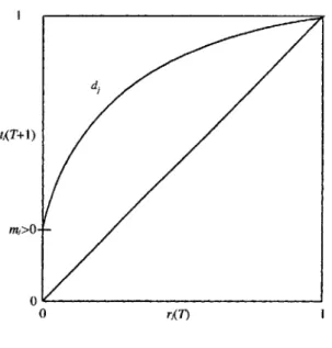
FIGURE1

Illustration of~

First, we assume that~(rj)is a simple diffusion of information process, i.e.

According to this diffusion process, knowledge about the existence of asset j can arise from three sources:rjis the percentage of people who remember asset j from last period." (l - rj) is the percentage of previously uninformed agents who might get informed by public information(m;>0 is called the "marketing coefficient") or by private information

(Wj~Ois called the "word of mouth coefficient"). Awareness of an asset only depends on last period's awareness of this particular asset, but it is completely independent of the level of awareness of any of the other assets. Hence, there are no "spill-over"-effects with respect to the information about the existence of an asset.

The diffusion process~(rj)is a simple monotone and strictly concave mapping from [0, 1]into [0, 1] which has a unique stationary point

r,

=

1.See Figure 1 for an illustration of~.26

Whereas ~(rj)is the percentage of agents being aware of assetj, aj is the "adoption coefficient" which determines the percentage of agents being aware of asset j and actually considering to participate in the market for this asset in the next period t+1. Again we suggest a simple multiplicative structure: ForK+(r) non-redundant let

wherejjrepresents a function measuring the relative "fitness" of an asset, whereas nj is

supposed to reflect the degree of innovation an asset is offering compared to the other existing assets. As a consequence, this definition of the coefficientsaj implies in general

25. Note that here we implicitly assume that agents do not forget.

26. Note that in the absence of the adoption coefficientQjthe number of people being aware of the financial

innovation will display an S-shaped time-path (upon iteration of our evolutionary process). This implication ofthe specification of the diffusion processdjis supported by the empirical literature on the diffusion of innovations (see

BETTZUGE & HENS FINANCIAL INNOVATION 505 that the transition function for an asset jeJis a non-trivial function of the entire partici-pation phase r: whereas

t;

only depends on rj> the adoption coefficients aj, and hence the transition functions gj, depend on r., ... ,rJ. Thus the transition dynamics is inherently multi-dimensional, and there are potential "spill-over"-effects between the assets.

The concept of fitness of an asset should reflect the expected gains from participating in this asset, and we take the trading volume to be an indicator for those gains." To fix ideas we will simply assume thatjj(Vj)

=

Vj' Itshould be noted that the assumed linearity of

f

will have a considerable effect on the results obtained in the following section, since it precludes complicated functional forms of the composite transition functiong.

There are at least three arguments made in the literature which support the assump-tion that the fitness of a financial asset is positively correlated with the volume it generates." Firstly, trading volume is often interpreted as a proxy for the liquidity of a financial asset (for a theoretical foundation of this argument see for example Hopenhayn and Werner (1996) or Pagano (1989a». Liquid assets are, ceteris paribus, considered to be more attractive to investors than illiquid ones for three reasons: They can better be real-ized at short notice (Grossmann and Miller (1988», they are subject to a reduced influence of strategic behavior-which can either be due to asymmetric information as in Kyle (1985, 1989) or Admati and Pfleiderer (1988), or due to imperfect competition as in Pagano (1989a)-and they are less volatile (see e.g. Pagano (1989b». Secondly, a number of studies have stressed that trading volume is a major factor governing the actions of financial intermediaries. Such intermediaries, for example exchanges or brokers, are often (directly or indirectly) compensated by some form of transaction fees which are portional to the trading volume; hence, these intermediaries attempt to find and to pro-mote such financial assets which generate high trading volumes. For models in support of this argument see for example Duffie and Jackson (1989), Cuny (1993), Hara (1995), or Bisin (1999)/9 Finally, a third argument can be made in favour of interpreting an asset's trading volume as its fitness: As Bikhchandani, Hirshleifer and Welch (1998) have pointed out, herding behaviour is an important phenomenon in the presence of bounded knowl-edge and asymmetric information. In this sense, high trading volume can here be inter-preted as a signal that an asset is widely and successfully used, and which therefore attracts new consumers who had so far not adopted this asset.

Finishing the specification of the transition function, the factor nir) is supposed to measure the degree of innovation in the payoffs of assetj relative to the other assets already established where nj(r)

=

1 if ~(r)

=

{j} or ~(r)

=

0. To be more precise, let a participation rate

r

be given and assume that ~(f) forms a non-redundant set of assets. Then one can decompose the payoff Aj for any asset jeJ into a spanned component S,

and an innovation component

l.i,

i.e. Aj ==

l.i

+Sj, where S, is the p-orthogonal projection

of Aj onto the span of the otherassets already traded at f. Say S,

=

LkEK+(f)\{j}Ak

ek,

where

{jis defined as the unique solution to the optimization problem.

27. Obviously, if the preceding trading volume was zero, then no trader was able to gain anything on that market. Moreover, the higher the trading volume the more gains, in general. Hence, the fitness function should be starting at 0 and being monotonically increasing.

28. Black (1986) evendefinesthe success of a financial innovation by the trading volume attracted. 29. Observe that-in order to keep things separate-we have not incorporated this effect into the "marketing coefficient"mj(which we assumed to be exogenous and fixed), but that we have rather amalgamated all

In the sequel we will assume that this "innovation" coefficient has the following simple shape

nj(r)

=

JII~W

+f3j(r)IISjW,

where f3ir)

=

rj/(rj+ LkeK+(;')\{j{klekl) if the denominator is different from zero, and f3j(r) = 1 otherwise

For a motivation of this specific assumption on nj observe that in a model with restricted participation the degree of "innovativeness" of an asset depends on two factors: On the one hand, and as acknowledged by the literature on financial innovation" it depends on the level to which assetj contributes to the spanning opportunities available in the economy. On the other hand, the degree of novelty of an asset depends on the relative participation in assetj compared to the participation in the other assets. This has already been pointed out by Black (1986) who stresses that the availability of well-estab-lished "cross-hedging" opportunities for a new asset is one of the major reasons for the failure of this asset. Our formulation of the functionnjtherefore measures the "spanning factor" by II~II,and captures the "cross-hedging" factor by introducing the coefficientf3. Regarding the properties of the function nj, note that f3jE[0, 1] and hencenjE[0, 1] by our normalization assumption

IIAj

II

=

1 for alljEJ. Moreover, njis non-decreasing in rj and continuously differentiable in r.31 Furthermore, for a p-orthogonal asset Aj, it is obtained thatnj =1 for all rjE[0, 1]. Finally, if Ajhas zero participation and is redundant to some assets with positive market participation, then nj

=

0. These properties ofnjare, in fact, the only properties which will be used to derive our general results. The examples given in Subsection 4.2 are computed using the specific function njdefined above.

3.2. Notions of stationarity and stability

We now first have to look for steady states of the evolutionary process. These are captured by the following notion of a fixed point of the transition mapping defined by g. Our notion of stationarity thus describes a situation of market participation rates (and trading volumes) that sustain themselves over time, allowing for both high participation in some assets and low participation in other assets.

Definition2. A participation phase FE[0,Ifis astationary equilibrium of the evol-utionary process

if

F

=

g(F).

From the definition of the transition function g it is obvious that r

=

(0, ... , 0) always is a stationary equilibrium.

We continue by investigating the stability of stationary equilibria by analysing which set of assets is robust with respect to some ongoing process of financial innovations. First, we define stability of a set of assets with respect to the further introduction of new assets, i.e.financial innovations.

Definition 3. A stationary equilibriumFE[0,I]J with

if

=

°

is evolutionarily stable with respect to the innovation of assetj

if

the following holds: There exists some £jE(0, 1)such that for every

1JE

(0,£j) the sequence r(t+1)=g(r(t)), with reO)=(F\j,1J),t=

30. See for example Duffle and Jackson (1989).

BETTZUGE & HENS FINANCIAL INNOVATION 507

ifJ1Ar\j, aj)nj(r)rj<1 otherwise

0, 1, ...converges to f. Moreover, a stationary participation phase isevolutionarily stable

if

it is evolutionarily stable with respect to any innovation.

Thus, a stationary participation structure is evolutionarily stable if the traded assets can be protected from "mutants" by certain entry barriers for the initial proportion of traders participating in the new asset markets. Note that if the uniform participation phase

r

=

(1, ... ,I) is a stationary equilibrium, it is also evolutionarily stable since no more entrants can appear.

Similarly, we ask whether some asset market "remains perfect", i.e. whether an asset market with complete participation has a tendency to return to the situation of complete participation if its participation rate is reduced slightly below I.

Definition4. A stationary participation phase

re

[0,I]J with

0

=1remains perfect with respect to assetj

if

the following holds: There exists some £jE (0, I) such that for everyijE (1 - £1' 1) the sequence ret+1)

=

g(r(t», with reO)

=

(f\j,ij), t

=

0, 1, ...converges to f. Moreover, a stationary participation phaseremains perfect

if

itremains perfect with respect to any asset.

A stronger stability requirement than evolutionary stability and remaining perfect is given by

Definition 5. A stationary participation phase fE[0,I]J is asymptotically stable with respect to the subsets of assets KcJ

if

there exists some e>

°

such that for every fE[0,I]J withij

=

0,jflk and withIIf -

fll

<

e

the sequence, ret+I)

=

g(r(t» with reO)

=

f,t

=

0, 1, ... converges tof. Moreover, a stationary phase is asymptotically stable

if

it is asymptotically stable with respect tok

=

J.

Note that participation structures which are asymptotically stable also are evol-utionarily stable and remain perfect for every asset j while the opposite implication in general fails to hold. The concepts differ, since evolutionary stability and remaining per-fect only require robustness with respect to changes in the participation rates of single assets while asymptotic stability considers small deviations from the market participation rate in any possible direction.

4. MAIN RESULTS 4.1. Analytical results

We first introduce specific one-dimensional functions h, for every jeJ, which serve to greatly simplify much of the following exposition. In fact, for everyjeJ and for every (fixed)r\jE[0,1]J -1 we define

hArj):= gj (r\1'rj)

={d.i(rj)' nj(r)' J1j(r\1' aj)' rj d.i(rj)

Thus h,is the one-dimensional function governing the dynamics ofrjif the partici-pation rates, r\j, of the other assets were to be kept fixed.Itwill turn out in the sequel that in spite of the potential spill-over effects present in the economy (due to the construc-tion ofnjandJ1jwhich may depend on the entire vectorr),all the results for the existence

o

o o

FIGURE2

Generic shapes of the function h, (Lemma 5)

and stability of stationary points derived below can be deduced from the shape ofhj'The following lemma shows that-except for irregular cases-hj essentially takes three possible shapes, which are depicted in Figure 2.

Lemma 5. Let jEJ and r\jE[O,I]J-I be given, and let Jij=Jiir\j,aj)' Then

hj (rj):=gj(r\hrj) has the following properties:

(i) hAn)

=

0. Furthermore, hAl)

=

1only ifnAr\hI)Jlj~l.

(ii) IfnAr\j, I)Jij<1then hj(rJ<rjfor every rjE(O,1]and hi(0)<1.

(iii) Ifnj(r\hl)Jlj> 1and mjnAr\j,O)/lj>1 then hj(1)

=

1,hi(0)> 1,and hArj)>r.for all rjE(0, 1).

(iv) If nj(r\h I)Jij>1and mjnj(r\h O)Jij<1then hj(l)

=

1,hi(0)<1,and there exists a uniqueijE(O, 1)such that hAij)

=

ij. Moreover, in this case,h,is differentiable at

fj and hi (ij )>1.

Proof

(i) This follows directly from insertingrj

=

0 and rj

=

1 into the definition ofhj' (ii) In this case

hAl)

=

4i(1)nAr\j, I)Jlj< 1, hence h,ends below the diagona1. Since therefore

hj(rj)~4i(rj )nAr\h rj)Jij' rj~4i(I)nj(r\j, 1)/lj' rj<rj,

it follows thath,never crosses the diagonal in the open interval (0, 1). Moreover, one easily computes the derivative at rj

=

°

as

hi(O)

=

4i(O)nj(r\}, O)Jlj< 4i(0)

=

mj~1.

(iii) Here, hj(l)

=

4i(1)

=

1 by construction. Now consider the function

ii

j defined as

ii

j (rj):=d,(rj)nj

v».

rj)/lj(r \j, aj)

for every rjE[0, 1]. Clearly,

ii

j is strictly increasing, sinced,is strictly increasing and njis non-decreasing. Under the assumptions stated it follows that

iiAO)

> 1. Hence,~(rj)> 1 for every rjE[O,1]. Noting thathj(rj)

=

min {hi(rj)' rh 4i(rj)} >rj for every rjE(0, 1), then proves that hj cannot cross the diagonal in the open interval (0, 1). Furthermore, the assumptions imply that hi(0)

=

mjnj(r\}, O)Jij>1.

BETTZUGE & HENS FINANCIAL INNOVATION 509

i=1, ...,I,

(iv) Again,hAl)=4i(l)= 1follows by construction. Now, for the functionJij defined

above, one obtains thatJij (0) < 1andJij (1) > 1.Hence, due to the strict monoton-icity ofJib there must be a unique point fjE(0, 1)such thatJiAfj)

=

1.But in this casehAfj)

=h

j

v» .

r,

=

fj,and

r,

is unique in (0, 1)as claimed.

In the case considered, the derivative ofhjat rj

=

1satisfieshj(l)<1.But then, at fj, h, must cross the diagonal from below. Since4i(fj)>fjimpliesaAfj)<1,it follows thathjis differentiable at

r..

Hence, hj (fj)>1.

II

To see what is driving this result consider the role of aj: Either it never becomes constant, then hiis stationary only inrj

=

o.

If, however, it does become constant then, in a neighbourhood of rj

=

1, hj is identical with 4i which has a simple shape and which strictly lies aboves the diagonal.

Therefore, Lemma 5 completely characterizes the possible shapes ofhj in all the cases

where mjnAr\b O)llj:t:1and n/r\j' 1)llj:t:1("regularity conditions"). Since we are only concerned with phases r\ j which are part of a stationary equilibrium, it suffices to show

that these regularity conditions are met for all stationary points. As the next proposition demonstrates, this is in fact true for almost all endowments m=(mt, ... , m/)EIR(S+1)/.

Lemma 6. For all endowment distributions, except for some set CclR(S+1)/ of

Lebesque-measure zero, the regularity conditions mjnj(f\b O)llj:t:Iand nj(F\j, 1)J.fj:t:1,where J.fj

=

Ilj(f\j, aj), hold at all stationary equilibriaFE[0, 1]J with

14(F) forming a non-redundant

set of assets.

Proof32 Let FE [0,I]Jbe a stationary equilibrium. As in the Market Partition Lemma, consider the GEl-economies GEI(F,K)

=

{IR(S+1>, A(F, K),

ur,

mi)f= I}' where A(F, K)is a submatrix of A, consisting only of assets jeK ~14(F) with positive participation rates. Equilibrium trading volumes are

*.

1

T I T

(1

. .)

81 ( m )

=

-:(A(F, K) OA(F, K)f A(F, K) 0 - ml - ylmll ,

r'

I(

/ . / . *.

where 1(=Li=I(l/yl) and ml=Li=".mll. Hence, 81!~) is a continuously differentiable

function for mEIR(S+1)/and rank dOl8

1 ( m )

=

IKI,

i.e. 81

(m)is "controllable" by t». Hence, b,y the parametric transversality theorem, for all

ca

except for a set C of measure zero, 85(m):t:0 so that the aggregate trading volume af(m)

=

L~=1Ie5(m)1

is continuously dif-ferentiable and controllable by m,i.e.rank dOl(af(m), ....a;(r»)

=

IKI.

Therefore, for all i», except for a set of measure zero, nAF)J.fj(F\j, af):t:1for alljEJ and for all K c;;,

14

(F). A similar argument can be applied for the second regularity con-dition mjnAr\b O)llj(F\j, af):t:1, noting thatnjis continuously differentiable inr\j.

II

The stability properties of the evolutionary process are determined by the eigenvalues of the Jacobian of the transition function g: [0,

If

-:>[0,

If

evaluated at the stationary equilibria. Therefore, we need to clarify whether g is differentiable at every stationary phase FE [0,

If,

where, as has been noted before, for stationary phases in the boundary of [0,

If

the derivative has to be taken only in any direction pointing to the interior of [0,

If.

Note that the transition function g need not be differentiable at a point where njvj= 1.

32. This proof uses some parametric transversality theorems (for a precise statement and a thorough dis-cussion thereof see Magill and Quinzii (1996».

Proposition 3. For all endowment distributions, except for some set C of measure zero, the transition function g:[0, If~[O,I]J is continuously differentiable at all stationary equilibrium phasesFE[0,If with 14(F)forming a non-redundant set of assets.

Proof By construction, d.i(rj) and nj(r) are continuously differentiable. Corollary 1 has demonstrated that the volume function vj(r) is continuously differentiable as well. Hence, it remains to argue that, generically in endowments, nj(F)vj (F)

=

nj(F)Jlj(F\h aj)f.j=t:-l for all stationary equilibria F under consideration. Now gAF)

=

f.j and nj(F)vAF)

=

1imply d.i(f.j)

=

f.jand, hence, f.j

=

1.Therefore, the claim follows as a corollary from the previous lemma.

II

After these preliminaries we can characterize stationary equilibria F in terms of properties of their coordinates f.j forjEJ.

Theorem 1. Suppose 14(F\j, 1)forms a non-redundant set of assets, and let F be a stationary equilibrium. Let Jlj

=

Jlj (F). Then

(i) f.j

=

1only

if

nj(F)Jlj~1.

(ii) Moreover, at F, let the economy satisfy the regularity conditions, i.e. let mjnj(F\j, O)Jlj=t:-l and nAF\h I)Jlj=t:-1. Then f.jE(0, 1)only

if

nAF\h O)Jljmj<1<nAF\h I)Jlj. Such a mixed participation phase is unique in(0, 1).

Proof A stationary equilibriumFE[0,If is a solution to the equation F=g(F),where gj(F)=min {I, nj(f)Jljf.j}d.i(f.j) for all j=1, ...,J. Hence, if F is a stationary equilibrium, then hAf.j)=f.j for every jEJ (where r., is held fixed). But then, the statements in the theorem follow directly from Lemma 5.

II

From Theorem 1, we get simple conditions for the stationarity of the two extremal participation structures, zero participation and complete participation in all assets, respectively.

Corollary 3.

(i) F=(0, ... , 0)always is a stationary equilibrium.

(ii) For any non-redundant set of assets K~J, a phase FE[0,I]J with r,= 1for every jEK is a stationary equilibrium only

if

nj(F)Vj (F)~1for everyjEK. Moreover

if

nj(F)vj (F)~1 for every jEK and f.j=

°

for every j'lK then F is a stationary equilibrium.

(iii) Let A be p-orthogonal. Then, for any non-redundant set of assets KcJ, a phase FE[0,I]J with f.j

=

1 for every je K is a stationary equilibrium

if

and only

if

a;~1. Moreover, f.jE(O,1) is part of a stationary equilibrium only

if

a;mj< 1, and a; f.j<1in which case

r,

in unique.

Proof Parts (i) and (ii) are obvious from Lemma 5 and Theorem 1. To see (iii) observe that ifA is p-orthogonal, then nj(f)

=

1 by construction and Jlj(F\j, a j)

=

a;by the proof of Lemma 3. Hence nj(F)Jlj= a;'

II

In order to determine the stability properties of stationary equilibria, we now com-pute the derivative of the transition function.

BETTZUGE & HENS FINANCIAL INNOVATION 511 Lemma 7. For any stationary equilibrium fE[O,Ifwith 14(f) non-redundant andfor almost all endowmentsOJwe get:

iff.j=o iff.j=1 (ii)

If

f.jE{a,I}andk:;:. j then drkgj(f)

=0.

(iii)

If

f.jE(0, 1)then drjgj (f)> 1.

Proof Recall that gAf)

=

dAf)aAf), where

«o»

=

f.j+ mAl - f.j)+Wjf.j(1- f.j) and aj(f)=min {I,nj(f)vj(f)} for every jEJ.

Compute

where

and

ifnAf)vAf)>1, k,jEJ.

(i) Suppose k

=

j and

r,

=

0. Then aAf)

=

°

since vj(f)

=

0. Moreover, for the same reason drjaj(f)

=

nj(f)drjvAf). By Lemma 4, drjvAf)

=

J1Ar\j, aj)' Hence, drjgAf)

=

mjnAf)J1j(r\h a j).

On the other hand, suppose k

=

j and f.j

=

1. Then aj(f)

=

1 and nj(f)vj(f)

=

nj(f)J1j>1 by Theorem l(i), so thatdrjaAf)

=

0. Hence,drjgj(f)

=

1 - mj - Wj'

(ii) Suppose k:;:.j. Then, drkl!.i(f.j)

=0, since

l!.i only depends on rj. IfnAf)vj(f)>1, thendrkaj(f)=0. Ifnj (f)Vj (f)<1, then aj(f)<1 and sinceris a stationary equili-brium withf.jE{a, I}, it must follow thatf.j

=

°

by Theorem l(i). But then,vAt) =

°

and, by Lemma 4,drkVj(f)

=

0, hencedrkgj(f)

=

0.

(iii) Suppose

'.JoE

(0, 1) is part of the stationary equilibrium. Observe that drjgAf)

=

hj (f.j) where

r

\j

=

(f., ... , f.j- .,

r,

+h . . . ,fJ ) is held fixed. Then

The-orem 1 (ii) and Lemma 5(iv) imply that drjgj(f)>1.

II

The stability properties of stationary equilibria are derived from Lemma 7 by appli-cation of some well known results of the Theory of Dynamical Systems. A stationary equilibrium is asymptotically stable if all the eigenvalues of the Jacobian of the transition function evaluated at the stationary point have absolute value less than 1 (see, for example, Devaney (1986)). Moreover, a stationary uniform participation phase f which is asymptotically stable with respect to 14(f) is evolutionarily stable with respect to the mutation of a new assetj~14(f) if the diagonal entry corresponding to this mutation has absolute value less than 1. This condition for evolutionary stability follows from Lemma 7. Consider a stationary point with fk =0. Since by Lemma 7,drkgj(f)=

°

for allj with f.jE{a, I}, the Jacobian matrixdrgis a diagonal matrix at any uniform participation phase, and therefore, in a small neighbourhood aroundf, the derivative ofg in the direction of k is given by drjgj(f). A similar argument applies for the stability with respect to small reductions of participation levels below 1,i.e.for an asset's property to remain perfect.

Therefore, we get the following stability properties:

Theorem 2. At any stationary equilibrium re{O, I}J with ]4(f) non-redundant, and

for almost all endowments 00, we get:

(i) Iff is asymptotically stable with respect to ]4(f) then

r

is evolutionarily stable with respect to the innovation of a non-redundant asset jrt.]4(f)

if

mjnj(f)J.1j<1. (ii) Iff is asymptotically stable with respect to ]4(f) then

r

is not evolutionarily stable

with respect to the innovation of a non-redundant asset jrt.]4(f)

if

mjnAf)J.1j>1. (iii) Iff with ij= 1 is asymptotically stable with respect to ]4(f)\{j} then the

partici-pation structure remains perfect with respect to assetj.

Moreover any stationary equilibrium f with ije (0, 1) for some j eJ is not asymptotically stable.

Proof First assume that fe{O, I}J. Then, by part (ii) of Lemma 7, the directional

derivative of g in the k-th direction is given by the k-th diagonal element of drg(f). Hence, part (i) of Lemma 7 together with Lemma 5 gives the stability conditions (i), (ii), and (iii). To show the last statement assume that f is stationary. and that there is some keJ such that fke (0, 1). Recall from elementary linear algebra that the trace of a matrix is equal to the sum of its eigenvalues. Part (ii) of Lemma 7 implies for every jeJ with je {O, I} that the j-th unit vector is a left eigenvector of drg(f) with corresponding eigenvalue drjgAf). Since furthermore drkgk(f) > 1 for k with fke (0, 1), at least one eigenvalue of drg(f) must be greater than one. Hencer is not asymptotically stable.

II

Moreover, as the next theorem shows, a stationary equilibrium with full participation in a complete set of markets is not only evolutionarily stable but also asymptotically stable.Ifthe economy happens to settle in a complete set of markets it cannot be unsettled by small perturbations to the participation rates.

Theorem 3. Any stationary equilibrium

re

{O, I}J with]4(f) forming a non-redundant

and complete set of markets is asymptotically stable.

Proof To demonstrate asymptotic stability first note that by Lemma 7, drg(f) is a diagonal matrix because by assumption of Theorem 3 for all jeJ either ij=

°

or ij= 1. Hence locally the transition function gdecomposes intoJ independent functions. There-fore f is asymptotically stable if every je]4(f) remains perfect and if

r

is evolutionarily stable with respect to any jrt. ]4(f). The former is indeed the case because for f = 1 the j-th diagonal element is 1 - mj - Wj which is smaller j-than one. The latter requires to extend gon a neighbourhood of

r

to redundant assets. Such an extension which keeps the utility maximization property of asset demand and which does not destroy the differentiability ofgis always possible, as the following simple example demonstrates.

Let j be such that j(]]4(f)

=

0 be a set of possible financial innovations, each of which is redundant to ]4(f), i.e.

Aj

=

LkeK+(;') A k

8{,

je

t.

N ow with reference to Definition 3 consider the recursion

rk(t+1)

=

r, -

Ljel8i,.,rAt), rj(t+1)= 1/(t+1)rAO),

with rk(O)

=

fk, t

=

0, 1,2, .k e ]4(f), with rAO)=

e.,

t=0, 1,2, ,jei.

BETTZUGE & HENS FINANCIAL INNOVATION 513 Note that limt~OO

=f. Finally note that for any such extension f is evolutionarily

stable because the innovation coefficient,nj(f), is zero for allj~/4(f). Hence,

r

is indeed asymptotically stable.

II

Finally, in the case of p-orthogonal assets the criterion for evolutionary stability is independent of the particular equilibrium.

Corollary 4. Let the assets be p-orthogonal. Then a stationary equilibrium re[0,I]J with /4(f) non-redundant is evolutionarily stable with respect to the innovation of asset j~/4(f)

if

afmj< 1.

If

afmj> 1, then f is not evolutionarily stable with respect to the inno-vation ofasset j. Moreover,

r

is asymptotically stable

if

and only it it is evolutionarily stable.

Proof By construction nAf)

=

1 for all jEJ if assets are p-orthogonal. Moreover, by Lemma 3, the equilibrium volume of trade of any asset is independent of the other assets' market participation. Hence, org(f)is a diagonal matrix, and its stability properties then are determined by its diagonal entries.

II

The simple stability properties of stationary equilibria derived in Theorems 2 and Theorem 3 and in Corollary 4 rely on two particular features of the transition process:

Firstly, whenever a stationary equilibrium r corresponds to a standard GEl-economy, i.e.whenever fE{O,I}, then f can locally be characterized by the one-dimensional dynam-ics described byh,for every jeJ.In particular, the stability of

r

only depends on the slope ofhjat r,

=0 and

r,

=

1. The derivative hj(O)depends on the marketing coefficientmj, the coefficient of asset j's trading volume J.1j(f\h a j), and the degree of asset j's "innovative-ness" nj(f\h0).If,for example, there is no marketingeffort." i.e. mjsmall, or if assetj is almost redundant(njsmall) or if it does not generate a sufficiently high trading volume (J.1j is small), then evolutionary stability with respect to assetj follows, i.e. assetj is a "failure". On the other hand, the derivative hj(l) will always be smaller than 1 since if ij

=1 is a part of a stationary equilibrium then

hj necessarily is identical to ~in a neigh-bourhood of 1 (for "regular economies",i.e. for almost all endowments), where dj(l)

=

1 - mj - Wj<1. But the fact that the cross-derivatives do not matter in this case (Lemma 7(ii» implies that assetj must be remaining perfect. Hence, any small reduction of market participation rates of assets in which there is full participation in the stationary equilib-rium will lead back to full participation.

Secondly, the economy cannot get stuck in a situation of mixed market participation, where potential spill-over effects might become relevant (i.e. where the cross-derivatives can be non-zero): In such a situation, eventually, and after any perturbation, every asset will either be adopted by the entire economy or it will disappear. As can be seen from the proof of Lemma 7(iii), this instability is implied by the important fact from linear algebra that the trace of a matrix is equal to the sum of its eigenvalues. Based on this observation, the lack of stability of mixed participation equilibria can be deduced from the shape of the one-dimensional functionshj-inspite of the fact that the transition function is multi-dimensional in any neighbourhood around the mixed participation equilibrium. As a consequence, the "standard" GEl-economies are the only stable stationary outcomes of the dynamical process modelled in this paper, and they are characterized by simple, locally one-dimensional, dynamics.

33. Itis commonly found in the empirical literature that marketing is among the key factors that distinguishes top performing products in financial services (see Cooper, Easingwood, Edgett, Kleinschmidt and Storey (1994».