Buyout prices in online auctions

Buyout Prices in Online Auctions

by

Shobhit Gupta

B. Tech., Mechanical Engineering (2002)

Indian Institute of Technology, Bombay

Submitted to the Sloan School of Management

in partial fulfillment of the requirements for the degree of

Doctor of Philosophy in Operations Research

at the

MASSACHUSETTS INSTITUTE OF TECHNOLOGY

June 2006

( Massachusetts Institute of Technology 2006. All rights reserved.

Author

...

'

''..Sloan

School of Management

cam

May 18, 2006

Certified

by...

_. 7.."~r~emie

Gallien

J. Spencer Standish Career Development Professor

Thesis Supervisor

Accepted

by ...

...

James B. Orlin

Edward Pennell Brooks Professor of Operations Research,

Co-director, Operations Research Center

OF TECHNOLOGY J L 2 4 2006

LIBRARIES

Buyout Prices in Online Auctions

by

Shobhit Gupta

Submitted to the Sloan School of Management on May 18, 2006, in partial fulfillment of the

requirements for the degree of

Doctor of Philosophy in Operations Research

Abstract

Buyout options allow bidders to instantly purchase at a specified price an item listed for sale through an online auction. A temporary buyout option disappears once a regular bid above the reserve price is made, while a permanent option remains available until it is exercised or the auction ends. Buyout options are widely used in online auctions and have significant economic importance: nearly half of the auctions today are listed with a buyout price and the option is exercised in nearly one fourth of them.

We formulate a game-theoretic model featuring time-sensitive bidders with in-dependent private valuations and Poisson arrivals but endogenous bidding times in order to answer the following questions: How should buyout prices be set in order to maximize the seller's discounted revenue? What are the relative benefits of using each type of buyout option? While all existing buyout options we are aware of currently rely on a static buyout price (i.e. with a constant value), what is the potential ben-efit associated with using instead a dynamic buyout price that varies as the auction progresses?

For all buyout option types we exhibit a Nash equilibrium in bidder strategies, argue that this equilibrium constitutes a plausible outcome prediction, and study the problem of maximizing the corresponding seller revenue. In particular, the equilib-rium strategy in all cases is such that a bidder exercises the buyout option provided it is still available and his valuation is above a time-dependent threshold. Our numerical experiments suggest that a seller may significantly increase his utility by introducing a buyout option when any of the participants are time-sensitive. Furthermore, while permanent buyout options yield higher predicted revenue than temporary options, they also provide additional incentives for late bidding and may therefore not be al-ways more desirable. The numerical results also imply that the increase in seller's utility (over a fixed buyout price auction) enabled by a dynamic buyout price is small and does not seem to justify the corresponding increase in complexity.

Thesis Supervisor: Jr6mie Gallien

Acknowledgments

I am deeply indebted to my thesis advisor, Professor Jr6mie Gallien, for his unwa-vering guidance, support and encouragement. His enthusiasm for research, attention

to rigor and detail, and limitless knowledge has been a constant source of inspiration guiding me over the last four years. He has been very generous with his time and very supportive of my efforts. Thank you, Jremie!

I would also like to thank my thesis committee members, Professor Stephen Graves and Professor Georgia Perakis, for their critical comments and suggestions that have greatly improved the quality of this dissertation. During my years at MIT, I have gained valuable teaching experience for which I am thankful to Professor J6r6mie Gallien, Professor Stephen Graves, Professor John Wyatt and Professor Roy Welsch who very kindly offered me tutoring positions. A very special note of thanks to Professor John Wyatt who gave me his car - owning a car has been a great convenience and luxury and has vastly improved my student life experience.

I spent a lot of time in my office at the ORC and am very thankful to my col-leagues for being such a fun group of people and an excellent source of help. I would specially like to thank Pranava Goundan and Raghavendran Sivaraman for their help with all my research problems, and Kwong Meng Teo, Dan Stratila and Alexandre Belloni for being great office-mates. Special thanks to Paulette Mosley, Laura Rose, Andrew Carvalho and Veronica Mignott for their superb administrative assistance and friendship.

Finally, I will like to thank Smeet for her love, friendship and care. Of course, this thesis would not have been possible without the unconditional love and support of my parents and sisters who have always believed in me and encouraged me. This dissertation is dedicated to my parents to whom I am eternally grateful for all the values they have instilled in me.

Contents

1 Introduction 13

1.1 Literature Survey ... ... 16

1.1.1 Literature on Online Auctions ... 16

1.1.2 Literature on Buyout Price auctions . . . ... 19

2 Market Environment and Auction Mechanism

25

2.2 Auction Mechanism ... 26

2.3 Model Discussion ... 28

3 Static Buyout Prices

33

3.1.1 Outcome Prediction ... 34

3.1.2 Equilibrium Refinements ... .. 45

3.1.3 Seller's Optimization Problem ... 54

3.2 Permanent Buyout Option ... 62

3.2.1 Outcome Prediction ... 62

3.2.2 Equilibrium Refinements . . . 74

3.2.3 Seller's Optimization Problem .. . . . .. 76

4 Dynamic Buyout Prices

79

4.1.2 Seller's Optimization Problem. 4.2 Permanent Buyout Option ...

4.2.1 Outcome Prediction.

4.2.2 Seller's Optimization Problem . . . . .

89 93 93 98

5 Empirical Analysis, Numerical Results and Comparative DiscussionlO5

5.1 Static buyout prices ... ... 105

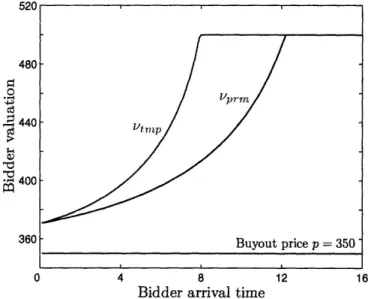
5.1.1 Equilibrium threshold valuation functions ... 106

5.1.2 Approximate temporary buyout price ... 107

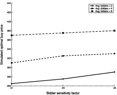
5.1.3 Temporary and permanent optimal buyout prices ... 108

5.1.4 Gain in seller's utility enabled by a buyout price ... 111

5.2 Dynamic buyout prices . . . ... 114

5.3 Empirical Analysis of Bidding Data . ... 117

5.3.1 eBay Data ... 120

5.3.2 Yahoo Data ...

...

.

123

6 Conclusion

A Appendix

A.1 Proof of Proposition 1 ... A.2 Expression for Et[max(v, v(2T)+l )1

A.3 Proof of Lemma 8 ... A.4 Proof of Lemma 10 ... A.5 Proof of Proposition 2 ... .

133 133 134 135 141 143 . .. . . .

...

...

...

...

...

List of Figures

2-1 Snapshot of an online auction webpage ... 28

5-1 Equilibrium threshold valuation in temporary and permanent buyout price auction . . . ... 106 5-2 Optimal temporary buyout price ( = 0.03) ... 109 5-3 Optimal temporary buyout price ( = 0.03) ... 110

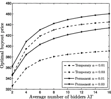
5-4 Optimal temporary and permanent buyout prices with impatient bid-ders . . . ... 111 5-5 Relative increase in seller's utility from a temporary buyout option

( = 0.03) ...

112

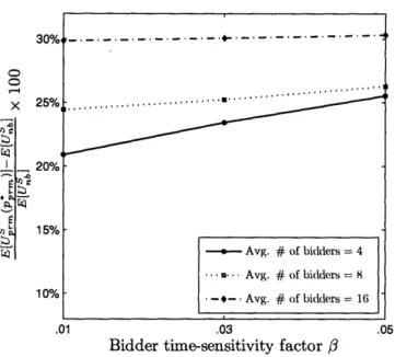
5-6 Relative increase in seller's utility from a permanent buyout option

(p = 0.03) ...

113

5-7 Relative increase in seller's utility from a temporary buyout option

(a = 0.03) ...

114

5-8 Relative increase in seller's utility from a permanent buyout option

(a = 0.03) ...

115

5-9 First activity time as a function of winning bid ... 121 5-10 Plot of mean first activity time with mean winning bid in a temporary

buyout price auction ... 124

5-11 Average bid time as a function of winning bid ... 125

List of Tables

3.1 Optimal buyout price in asymptotic regimes ... 59

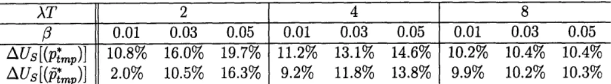
5.1 Percent utility increase achieved by temporary optimal and

approxi-mate buyout price .. . . . ... ... 108

5.2 Utility increase achieved by fixed and dynamic temporary buyout prices116 5.3 Utility increase achieved by fixed and dynamic permanent buyout prices16 5.4 Summary of auction data with wb < $30, bp > 1.25, and b > 0.8 . 121 5.5 Mean first activity time for different winning bid cutoffs ... 123 5.6 Summary of auction data with wb > $100, _Sp bP > 1.25, and b > 0.8. _{- ·} bp 125

Chapter 1

Introduction

As they were initially conceived during the last decade of the previous century, online auctions were arguably suffering from two perceived drawbacks relative to posted price mechanisms: waiting time and price uncertainty. In order to render these auctions more attractive to time-sensitive or risk averse participants, many auction sites have since introduced a new feature known as a buyout option, which offers potential buyers the opportunity to instantaneously purchase at a specified price an item put for sale through an online auction. Indeed Mathews (2003b) notes that "one of the reasons eBay introduced [the buyout] option is that buyers wanted to be able to obtain and sellers wanted to be able to sell items more quickly". Augmented with this option, an online auction thus becomes a hybrid between an electronic catalogue and a traditional auction.

Buyout options are now widespread and have significant economic importance: in the fourth quarter of 2003 alone, fixed income trading (primarily from the buyout option "Buy It Now") contributed $2 billion or 28% of eBay's gross annual merchan-dise salel; other examples of buyout options include Yahoo's "Buy Price", Amazon's "Take-It" and uBid's "uBuy it!". Remarkably, buyout options in these large auction sites currently differ in one important aspect: eBay's "Buy It Now" option disappears as soon as a regular bid above the reserve price is submitted, so it is called temporary; in contrast Yahoo, Amazon and uBid's options remain until they are exercised or the

1

auction in which they are featured ends, so they are called permanent (Hidv6gi et al. 2003).

These observations motivate in our view the following questions: What is the benefit associated with using a buyout option for a seller in an online auction? How should the buyout price be set when doing so? Should a temporary or a permanent buyout option be used? We design a game-theoretic model to answer these questions in a stylized setting - the market environment and the auction mechanism we consider are specified in §2.1 and §2.2 respectively, and we discuss the realism of the model in §2.3. For this model, for both the temporary and permanent buyout option an equi-librium in bidder strategies is characterized and the associated seller's optimization problem is discussed. We extend next our analysis with the goal of answering the following question: while all existing buyout options we are aware of rely on a static buyout price (i.e. with a constant value), what is the potential benefit associated with using instead a dynamic buyout price that varies as the auction progresses? The main contributions of our research can be summarized as following:

1. Analysis for temporary and permanent buyout price auctions - We characterize equilibrium strategies for temporary and permanent buyout price auctions in §3.1.1 and §3.2.1 respectively, and analyze their robustness to perturbations in strategy and payoff space (§3.1.2 for temporary and §3.2.2 for permanent). We also conduct a simple empirical analysis, described in §5.3, to validate the predictions of these strategies using bidding data from actual online auctions. For limiting regimes of bidder arrival rate, and bidder and seller time sensitivity, we derive optimal buyout prices for both options (§3.1.3 and §3.2.3).

2. Comparison of temporary and permanent buyout option - Our numerical exper-iments, discussed in §5.1, suggest that the seller's expected discounted revenue derived from an optimal permanent buyout option is larger than that obtained with an optimal temporary option. Furthermore, the relative attractiveness for the seller of a temporary buyout option decreases with the expected number of bidders, whereas it increases in the case of a permanent option. The

equilib-rium analysis however implies that the permanent option promotes late bidding -- a fact that is also corroborated by bidding data obtained from online auction websites - which may negatively impact the seller's revenue.

3. Dynamic buyout price - We analyze temporary and permanent dynamic buyout price auctions - §4.1.1 (resp. §4.2.1) focuses on outcome prediction in the tem-porary (resp. permanent) case and §4.1.2 (resp. §4.2.2) discusses the resulting optimization problem. Our numerical experiments, discussed in §5.2, suggest that the increase in seller's utility (over a fixed buyout price auction) enabled by a dynamic buyout price is small and does not seem to justify the corresponding increase in complexity - dynamic prices will be difficult to implement and may be too complex for bidders to understand.

Chapter 6 contains the concluding remarks, and all proofs omitted from the main text are included in the Appendix.

The results (1) and (2) can assist a seller in selecting the appropriate auction mechanism (including the optimal buyout price, if required) based on his preferences and the market environment for the product. The above results could also have important auction design implications: for example, the outcome prediction for a permanent buyout price auction advocates using an auction mechanism which would allow bidders to submit "last-minute" bids in advance hence avoiding the hassle of tracking the auction to place a bid near its end. This could however convert the

auction into a sealed bid second-price auction which may not be desirable; see Roth and Ockenfels (2002) for a discussion on introducing the sniping option in an auction. The conclusion (3) suggests that there is little advantage for the seller of introducing a buyout option with time-varying price.

The following section in this Chapter reviews literature on auctions and buyout prices.

1.1 Literature Survey

Auctions, in many different forms, are very widely used; a historical sketch of the use of auctions is provided by Shubik (1983) - one of the most famous being an auction of the entire Roman empire in AD 193. More recently government contracts, United States Treasury bills, cars, arts and antiques have been auctioned (see Klemperer (1999)). With the advent of online auctions, the list of items sold by auction has ex-panded to include software, collectibles, electronic items, used books, concert tickets, furniture, and almost everything else2 (also see Lucking-Reiley (2000)).

As a consequence of their importance and popularity, there is a significant body of theoretical literature on auctions. A comprehensive but somewhat dated bibliography of auction literature is provided in Stark and Rothkopf (1979) while more recent surveys include Milgrom (1985), Milgrom (1989) and Klemperer (1999). McAfee and McMillan (1987) discuss developments in the theory of bidding mechanisms restricting to models analyzing, like we do, a single isolated auction. A critical discussion of available models aiding competitive decision making in auctions- bidding strategy for bidders and auction design for sellers - is presented by Rothkopf and Harstad (1994).

1.1.1

Literature on Online Auctions

Introduced in 19953, online auctions have gained tremendous popularity - eBay, ar-guably the biggest online auction website, had 135 million registered users and a gross merchandize volume, which is the total value of everything sold on eBay, of $34.2 billion in 20044. Lucking-Reiley (2000) traces the development of online auc-tions describing transaction volumes, types of auction formats used, type of goods auctioned, fee structure and the business model of various auction websites. There has been much recent research activity seeking to answer the many new questions posed by the emergence of online auctions; Pinker et al. (2003) characterize the state

2

http://en.wikipedia.org/wiki/Ebay

'Lucking-Reiley (2000)

4

of research and present many open problems in this field.

Online auctions have several unique characteristics - for instance, unlike tradi-tional auctions, a bidder in an online auction usually faces a random number of bidders; in addition, online auctions are typically longer in duration. These features impact bidder behavior raising new theoretical issues, which many papers seek to answer. Taking a dynamic programming approach, Bertsimas et al. (2002) develop a computationally-feasible algorithm to determine the optimal bidding strategy for a potential bidder in a single unit auction assuming that bids from other bidders are generated from a probability distribution which can be estimated using publicly available bidding data. They also extend their results to multi-unit auctions. Ariely and Simonson (2003) analyze bidding behavior focusing on two key aspects affecting the decision making process: value-assessment and decision dynamics. They discuss the effect of these two factors on bidder behavior at three key stages of an auction: (a) beginning of the auction (bidder decides whether to participate or not), (b) bid-ding during the auction and (c) bidbid-ding at the end of the auction. Park et al. (2005) build an integrated model, based on bidders' willingness to pay at any given auction round, of bidding behavior incorporating three main factors: which bidder placed a bid, the timing of the bid and its amount. Similar, in spirit, to our model, Carare and Rothkopf (2005) assume that bidders incur a fixed cost of waiting and returning later to the auction. Unlike our research, however, they analyze a Dutch auction mechanism deriving, in a simple two-bidder, two-valuation framework with transac-tion costs, pure- and mixed-strategy Nash equilibria in bidder strategy in a Dutch auction with a linear price function.

In a series of papers, Roth and Ockenfels analyze last-minute bidding in online auctions. Roth and Ockenfels (2002) and Ockenfels and Roth (2002) provide empirical evidence of late bidding and give strategic and non-strategic hypotheses justifying the phenomenon while Ockenfels and Roth (2005) show that last-minute bidding can occur at equilibrium in fixed price auctions if very late bids have a positive probability of being rejected. In all their studies, they observe that auctions with a floating deadline (see §2.3 for definition) experience lesser last-minute bidding than

fixed deadline auctions. Taking a different approach, Bajari and Hortacsu (2003) rationalize late bidding by considering a model with common values where bidders have an incentive to hide their private information by bidding at the last-minute.

Other aspects of online auctions are addressed by Segev et al. (2001) who model an online auction as a two-dimension Markov chain (the two dimensions being the current price and the number of bidders) to estimate the final selling price of a product. While a significant number of online auctions offer multiple units, literature analyzing multi-unit online auctions is fairly limited. In two papers Bapna et al. (2000) and Bapna et al. (2001) study bidding strategies in multi-unit auctions classifying bidders as opportunists, participators and evaluators based on when and how often they bid. Pinker et al. (2001) formulate a dynamic program for solving the problem of allocating inventory across several multi-unit auctions. They extend their model to develop a framework where information from earlier auctions is utilized to update seller's beliefs about bidder valuations and consequently improve the lot-sizing decisions.

Publicly available bidding data on auction websites has led to a number of empir-ical studies on online auctions. Kaufmann and Wood (2004) investigate factors that make bidders pay more for exactly the same item and find that items sold on week-ends, items with a picture and items sold by experienced sellers tend to sell at higher prices. A similar study by Lucking-Reiley et al. (2000) concludes that the auction selling price is higher when the seller has higher feedback ratings and the auction is longer. Several other papers including Houser and Wooders (2005), Melnik and Alm (2002), Ba and Pavlou (2002) and McDonald and Slawson (2002) study the effect on seller's feedback rating on auction outcome and conclude that seller ratings positively affect the selling price. Durham et al. (2004) study the "Buy-it-Now" option offered on eBay and find that seller reputation also has a significant impact on buyout price auctions - sellers with higher reputation are more likely to offer the buyout option and, the probability of option exercise increases with seller reputation. In another study, comparing auctions with online catalogs Vakrat and Seidmann (1999) find that, on an average, an item sells at significant discount (between 25% - 39%) when offered via an auction as opposed to a fixed-price mechanism.

1.1.2 Literature on Buyout Price auctions

While the literature on auction theory, online and otherwise, is large, existing research work on buyout prices is recent and relatively limited. Indeed, the comprehensive 1999 survey of the auction literature by Klemperer (1999) makes no mention of buyout prices, and while Lucking-Reiley (2000) observes the use of buyout prices in his 2000 survey of internet auction practices, he points out that he is "[...] not aware of any theoretical literature which examines the effect of such a buyout price in an auction."

Most papers written since on buyout prices consider models where, in contrast with most actual online bidding interactions, the number of bidders is known in ad-vance to all participants. Studying such a model with two risk averse bidders having two possible valuations for an item, Budish and Takeyama (2001) show that augment-ing an English auction with a permanent buyout price can improve the seller's profit. Kirkegaard and Overgaard (2003) investigate the impact of a permanent buyout op-tion when two bidders with multi-unit demand face two sequential aucop-tions of one item each. In the presence of two competing sellers they find that the one running the first auction benefits from using a buyout option. When a single seller runs both auctions, they show that his total revenue increases if bidders expect him to use a buyout option in the second auction. In contrast, we consider an auction for a single item run by a monopolistic seller, so that our model does not offer any insights on the issues of competition between sellers, sequential auctions and multi-unit demand.

Other papers still assume that the number of bidders is known to all, but allow that number to be arbitrarily high. In a model with n bidders, Reynolds and Wooders (2003) focus on the effect of bidder risk aversion on seller revenue in auctions with a buyout price (temporary or permanent). For either type of buyout option they find that with risk-averse bidders an auction with the optimal buyout price increases the seller's revenue. Hidv6gi et al. (2005) also find that, ill the presence of risk aversion by either the bidders or the seller, such buyout price does increase the seller's revenue. However in their model, where participants are not time-sensitive, bidders' utility does not increase through the use of the buyout option. In a series of three papers

investigating variations of the same basic model, Mathews (2003b), Mathews (2004) and Mathews (2003a) focuses instead on the temporary buyout option. Specifically, he considers a fixed number of time-sensitive bidders with different arrival times, and explicitly captures the fact that early bidders may prevent later ones from exercis-ing the option. He shows that a risk averse or time-sensitive seller facexercis-ing either risk neutral or risk averse bidders will choose a buyout price ensuring that the buyout option is exercised with positive probability; he also finds that, depending on the val-uation distribution, the buyout option either makes all bidders weakly better off, or low valuation bidders weakly better off and high valuation bidders strictly worse off. Note that we do not investigate bidder welfare in the present paper. By assuming a deterministic number of bidders, the papers mentioned above assume that every bid-der knows with certainty upon his arrival how many competing bidbid-ders have already arrived and how many others are yet to come before the auction closes, which we believe to damage realism.

Furthermore, of all the papers analyzing buyout prices cited so far, the papers by Mathews are the only ones that capture, as we do in our model, the timing of bidder arrivals. That is, all others do not model the sequence in which bidders come to the auction site, and thus ignore the impact of each bidder's arrival time on his strategy. This is crucial as auction duration (and indeed the bidder arrival time) is an important factor affecting bidder participation strategy in buyout price auctions as illustrated by Wan et al. (2003) who, in a survey conducted by them, find that "38.7% respondents agree that the duration of an auction is a consideration in choosing the buyout option. 25% of the respondents replied that an auction with a long duration

(7 to 10 days) encourages them to use the "Buy It Now" option". The importance of time sensitivity of auction participants on buyout exercise is also confirmed by eBay - its user guidelines state the reduction in waiting time as the very first reason why both sellers ("Sell your items fast.") and buyers ("Buy items instantly") would want to use their buy it now features) - and, more generally, by the discussion forums of experienced online auction users; below we list several examples:

5

"This guide is for people that are tired of losing auctions at the last second or for people who are just in a hurry to get their item. By using the Buy-It-Now option, you can quickly find the best price for the item you are searching for." - Reviews and Guides, eBay (2005)

"One of the best features to come along in quite awhile is eBay's "Buy It Now" feature. This allows bidders to buy it immediately for a price that you set. It's great for buyers who don't want to wait days until an auction ends to see if theyve won. Sellers also benefit. I have sold items within a half an hour by offering the "BIN" option."6

"You can also sell in "Buy It Now" mode, where you establish a fixed price, and the "auction" ends as soon as someone agrees to pay that price. The fees are [t]he same as with standard auctions, but you could sell multiple copies of the same item in the time it would have taken you to run a single "standard" auction. [...] It's also good when you don't want the delays of standard auctions or the uncertainties of a variable auction price." - Seltzer (2004)

"Neither you nor the buyer needs to wait for the end of an auction cycle - you get your payment sooner, and buyers get their merchandize faster. This is a great way to move more merchandize, especially if you have a product that's in demand."7

Moreover, by assuming that all bidders can potentially exercise the buyout option irrespective of when they arrive, these papers do not capture a key feature of buyout price auctions - a bidder arriving earlier can make the buyout option unavailable to subsequent bidders by either exercising it (for both temporary and permanent option) or placing a bid in the auction (for the temporary option only). This leads to a material difference as we exhibit robust equilibrium strategies where bidders arriving earlier in the auction do bid/buyout immediately on arrival.

6http://auction.lifetips.com/subcat/69131 /selling/special-features/index.html 7

A model that ignores the arrival time of bidders also fails to capture the timing of bids placed in the auction. This is crucial as last-minute bidding and, in general, the timing of bids in online auctions has received considerable attention from both theorists - Roth and Ockenfels (2002) provide strategic and non-strategic hypotheses justifying late bidding - and practitioners - there are special softwares like eSnipe and Last Minute Bidder8 which allow bidders to place bids at the last minute. Also, auction sites frequently implement auction mechanisms that discourage late bids -for example, Amazon and Yahoo use a floating auction deadline that automatically extends if a bid is placed near the end of the auction; Amazon also offers a first bidder discount of 10% to promote early bidding. Despite the importance of bid timing, most of the literature analyzing bidder behavior in buyout price auctions either assumes exogenous bidding times (Caldentey and Vulcano (2004), cited below) or neglects the issue of bid times altogether (Budish and Takeyama (2001), Kirkegaard and Overgaard (2003), Reynolds and Wooders (2003), Hidv6gi et al. (2005)). In contrast, the time when bidders act after their arrival is endogenous in our model, and we find in fact that with a permanent buyout option buyers submitting regular bids are likely to do so only at the very end of the auction.

While the papers cited above analyze models with a deterministic number of bidders, Caldentey and Vulcano (2004), who consider a multi-unit auction with a permanent buyout option, assume like we do that bidder arrivals follow a Poisson process whose future outcome is not known to participants. In addition, they also assume that auction participants are risk-neutral and time-sensitive, and use in fact the exact same utility functions we do. Unsurprisingly, they find, as in our research, that bidder strategies characterized by a threshold depending on arrival time and buyout price form an equilibrium. However, there are important differences between their work and the analysis we develop for the permanent buyout option: The model in Caldentey and Vulcano (2004) assumes that bidders are only informed about the initial number of units and not the number of units remaining. In the single-unit auction we investigate, this would correspond to bidders not knowing whether the

8

item listed is still available or not. We assume instead that bidders have access to this information, which is a material difference since the specific threshold strategy we obtain as a result is different. In addition, as discussed above Caldentey and Vulcano (2004) assume bidders to act immediately (bid or buyout) upon their arrival. We do not however consider the multi-unit case here.

In summary, of all the papers cited above that analyze buyout prices, only Math-ews (2004) models the arrival time of bidders and considers endogenous bidding times. It however assumes a deterministic number of bidders and only analyzes the tempo-rary buyout option. Reynolds and Wooders (2003) - which as we pointed out ignores the impact of arrival and bid times - is the only paper we are aware of which at-tempts to study like we do both temporary and permanent buyout options in the same framework. Also, our model features more realistic information structure and strategy space than all others discussed, and we believe to be the first to provide an analysis of dynamic buyout prices.

Chapter 2

Market Environment and Auction

Mechanism

In this chapter, we first describe our game-theoretic model, focusing on the market environment in §2.1 and the auction mechanism in §2.2. We then discuss its realism in §2.3.

2.1 Market Environment

We consider a monopolistic seller opening at time 0 a market for one item. From that point on, he faces an arrival stream of potential buyers (or bidders) which is non-observable per se, but is correctly believed by all participants to follow a Poisson process with a known, exogenous and constant rate A. Bidders valuations (or the prices at which they are indifferent between purchasing the item and not participat-ing in the market) are assumed to follow an independent private values model - see Klemperer (1999) for background. Specifically, each bidder has a privately known val-uation, and all other participants initially share the correct belief that this valuation has been drawn independently from a distribution with cdf F and compact support [v, ] (define m = - v).

the seller when earning revenue R at time T is assumed to be

US(R, r) e-"R,

(2.1)

where ac > 0 denotes his time discounting factor.

Likewise, a bidder arriving at time t > 0 with valuation v E [v, v] who purchases the item at time T > t for a payment of x gets utility

U(v,

where p > 0 denotes his time discounting factor, assumed to be the same for all bidders. A losing bidder is assumed to derive zero utility from the market.

2.2 Auction Mechanism

The basic market mechanism we consider is a second-price auction with a time-limited bidding period [0, T]. That is, any bidder arriving at time t E [0, T] may submit a bid at any time in [t, T], provided it is larger than any other he may already have submitted (i.e. bidders are not allowed to renege on their purchasing offers). At time T, the item is sold to the highest bidder who pays then a price equal to the second highest bid; if only one bidder has submitted a bid by T the item is sold to him for a price of v, and if there are no bids the item is not sold. Note that the lower bound of the distribution support v thus effectively corresponds to a publicly advertised minimum required bid (any bids lower than v are ignored).

In addition to all the other information described previously, every bidder is as-sumed to know at every time r subsequent to his arrival the value of I., defined as the payment that would be made by the winning bidder if the auction were instead terminated at T. That is, I, is equal to (i) the second highest bid submitted over [0,

r]

allow bids below the current second highest bid to be placed in the auction unlike most auction sites. Notice that this does not affect the utility of either the bidders or the seller: such a bidder gets zero utility (neglecting his bidding cost) whether he bids or not while bids placed below the second highest bid clearly do not affect the seller's revenue.

The basic auction mechanism just defined (or a closely related version of it) is investigated for example in Vakrat and Seidmann (2001) and Gallien (2006). The critical extension that we study in the present paper is the upfront addition by the seller of a buyout price p, either temporary or permanent. Any bidder may exercise that buyout option at any time between his arrival and the end of the auction T, provided the option is still open then; this amounts to purchasing the item instan-taneously at a price of p, effectively terminating the auction. A temporary buyout option remains open from the beginning until its exercise or the first time that a regular bid is submitted by any bidder, while a permanent buyout option remains open until its exercise or the end of the auction. In line with observed practice, we assume that all participants know at any point in time whether the buyout option is still open.

Notice that we assume that bids higher than the buyout price can be placed in the auction. While this is in line with practice - for instance eBay and Yahoo allow bids above the buyout price - these websites do recommend that bidders must bid lesser than the buyout price. For example, a help page on Yahool suggests bidders to " [..] make sure to place your maximum bid below the buy price amount." Similarly, placing a bid higher than the buyout price on eBay leads to the following warning

"Your maximum bid is above or equal to the Buy It Now price. We recommend you simply purchase the item via Buy It Now." Notice that, even when the buyout option is available, a bidder with valuation higher than the buyout price may find it optimal to bid in the auction if he believes that he is likely to face very little competition from other bidders, and, as a consequence, he will be able to obtain the product at a price much lower than the buyout price (since the second highest bid is likely to be lower).

While we assume in Chapter 3 that the buyout price p remains constant through-out the auction, we study dynamic buythrough-out prices in Chapter 4. In the dynamic ex-tension we consider then, the seller commits upfront to a function of time [p(t)]t[,,T] describing the evolution of the buyout price (either temporary or permanent) over time, and that function is known to all bidders.

2.3 Model Discussion

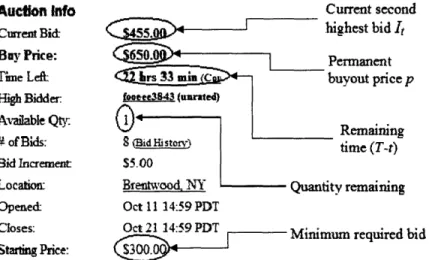
Our model is motivated by the online auctions occurring on large auction sites such as eBay and Yahoo; in that spirit Figure 2-1 includes a screenshot made on October 20, 2004 of an actual ongoing auction, along with pointers to the quantities in our model representing some of its features. As can be seen in that example the buyout option is still open although eight regular bids have already been submitted, indicating that it is permanent as opposed to temporary.

Auefoin Info Current second

Current Bid-Buy Price: Tine Left: High Bidder: vailable Qty: 4 of Bi:ds Bid Increment Locaiom: ighest bid It 'ermanent ~uyout price p Remaining time (T-t) v remaining Opened: Oct 11 14:59 PDT

Closes: Oct 21 14:59 PDT Minimum required bid v

Starting Price:

Figure 2-1: Snapshot of an online auction webpage

We first comment on our allocation mechanism. Online auction sites now typically feature "proxy bidding" systems, allowing bidders to enter the maximum amount they are willing to pay for the item. The system then submits bids on behalf of the bidder, increasing his outstanding bid whenever necessary and by as little as possible to maintain his position as the highest bidder, up until the maximum amount stated

is reached2. As observed by Lucking-Reiley (2000), an online auction with a proxy bidding system effectively amounts to a second-price auction, the payment mechanism we assume.

For the closing rule, we assume a hard bidding expiration deadline similar to the one used on eBay, whereas some other sites such as Amazon use instead a floating deadline that automatically extends (within some limits) whenever a new bid close to the current deadline is submitted. As pointed out in Roth and Ockenfels (2002), this difference is material and eBay-like hard bidding deadlines account for a demonstrably higher concentration of bids near the end of the auction. In principle, our model allows to predict such surge of bids shortly before the end, because while we assume exogenous bidder arrival times, their bidding times are endogenous. In fact, our analysis in §3.2.1 confirms the intuition that last-minute bids seem more likely with a permanent buyout option than with a temporary one. However, our model does not capture some of the important reasons why last-minute bidding may occur: presence of inexperienced (irrational) bidders; possibility that late bids may not reach the auction site due to network transmission delays; informational value of bids when the item being sold has a common value component... while we refer the reader to Roth and Ockenfels (2002) for an excellent discussion and empirical study of this phenomenon, we argue that factors such as the loss of last minute bids due to network transmission capacity and the presence of inexperienced bidders may not remain as prevalent in the long run, partly justifying these modeling choices (otherwise primarily motivated by tractability considerations). As a result, truthful and immediate bidding is a weakly dominant strategy in the model we assume for an online auction without a buyout option.

Another feature of the market mechanism we consider is the possible presence of a publicly announced minimum required bid, denoted "Starting Price" in Figure 2-1, effectively captured in our model by the lower bound v of the valuation distribution support. Note that this is distinct from what some auction sites (such as eBay) call a

"reserve price", which is likewise set by the seller as a minimum selling price for the 2_{See http://pages.ebay.com/help/buy/proxy-bidding.html}

item but, in contrast with the minimum required bid we use, is not publicly announced - when used by the seller, bidders are typically only informed that a reserve price has been set for the auction, and whether or not it has already been met by any of the existing bids. We assume that the seller does not use such concealed reserve price, in part because this would entail some inference of its value by the bidders, and may lead to further strategic interactions in the form of post auction negotiations between the winning bidder and the seller.

Several limitations of our analysis also stem from the market environment we consider. Our assumption that bidder arrivals follow a Poisson process seems more realistic than assuming that the number of bidders is known to all with certainty, and is partly justified by the classical Palm limit theorem on the superposition of counting processes. Nevertheless, the assumption that its arrival rate is constant and known to all participants (common to all other auction models assuming Poisson bidder arrivals that we are aware of) is still a strong one. In practice, the arrival rate of potential bidders to an auction could be variable; in particular, there may be a high concentration of bidder arrivals at the beginning of the auction - such an arrival process, for instance, can occur on auction websites, like eBay, that allow bidders to track newly introduced auctions. The high arrival rate of bidders at the start of the auction could be modeled by assuming that bidders arrive as a non-homogeneous Poisson process with a high arrival rate at the beginning of the auction; while this model is not analyzed in this thesis, our intuition suggests that most of the insights of our work will also be applicable to such a model. In practice, the arrival rate of bidders to a specific auction could also be endogenous, and depend for example on the bidding activity it has generated to date; it would also be influenced by factors such as advertising, the presence of a reserve price, the seller's feedback ratings, the presence and quality of photographs describing the item, etc. Our assumption of a constant known arrival rate saliently implies that bidders, including those arriving early in the auction when only little bidding history is available, correctly synthesize the impact of these factors when estimating how many competing bidders they are likely to face.

In reality, the estimations of both the arrival rate of competing bidders and the distribution of their valuations may differ among participants. Intuition suggests however that the items for which sellers are likely to use a buyout price that will be exercised with some non-negligible probability should coincide with those for which relatively substantial historical transaction data is available - this is also supported by the results in Gallien (2006) showing the lower robustness of fixed prices relative to auctions in the presence of market uncertainty. Because large auction sites make the same extensive historical transaction data available to all participants, our assumption of common beliefs seems legitimate as a first approximation in our view. We also observe that the lower bound v of the valuation distribution support may correspond in our model to a requested starting price, which (as can be seen on Figure 2-1, see also discussion of reserve price above) is announced to all participants.

The structure assumed here for the utility functions of the seller and the bidders is also used for example in Caldentey and Vulcano (2004) and Gallien (2006), and reflects a priori the proposed time sensitivity and risk neutrality of participants. While all the results in the paper have been derived for auctions with risk neutral participants, they can be easily generalized for risk averse auction participants - see §3.1.1 for a detailed discussion. The exponential time discounting that we assume for the seller applies to a monetary income, so that his utility can be interpreted as a straightforward net present value. As for the bidders, their exponential time discounting applies to the difference between their valuation for the item and their payment; this plausibly represents how a bidder may evaluate various actions (e.g. exercising the buyout option or submitting a regular bid) with different waiting time implications. Finally, our assumption that all bidders have the same time discounting factor is also a strong one, since bidders in online auctions are frequently end-consumers who are unlikely to share a single objective metric such as target ROI or reference interest rate when

assessing their dislike of waiting.

In summary, while our model does capture some of the key features of an online auction, there are some others that it does not reproduce as faithfully. We point out that an actual online auction is inherently a complex and random process involving

multiple heterogeneous bidders with various incentives and rationality levels inter-acting in a dynamic manner. As such, any tractable analytical model designed to predict its outcome (including ours and every other one described in the literature) must necessarily rely on fairly restrictive assumptions. Given our primary research objective of understanding the differential impact of temporary and permanent buy-out prices, we observe that several of these assumptions (e.g. common beliefs, bidder arrival process) may not specifically impact our model predictions when one type of buyout option is used as opposed to the other. From that perspective, we find it reassuring that our results rationalize some of the actual practices of auction sites using buyout options (see Chapter 6).

Chapter 3

Static Buyout Prices

In this chapter, we analyze auctions where the price of the buyout option remains fixed throughout the auction. We analyze a temporary buyout option in §3.1 and then, in §3.2, discuss a permanent buyout option.

3.1 Temporary Buyout Option

It is assumed for this section that the seller uses a fixed temporary buyout price p which disappears if a bid above the reserve price is placed in the auction. We characterize an equilibrium in bidder strategy for a temporary buyout price auction game (§3.1.1), analyze the robustness of the strategy (§3.1.2), and formulate the seller's optimization problem and discuss its solution in some asymptotic regimes (§3.1.3).

3.1.1

Outcome Prediction

For any bidder arriving at time t with valuation v, consider the following family T[.] of threshold strategies:

Buyout at p immediately if buyout option available and v > v(t) T[v](v, t) : Bid v immediately if buyout option available and v < v(t),

Bid v at any time in [t, T] otherwise

(3.1) where v: [0, T] - [, v] is a threshold valuation function. In the following we use the same notation for a strategy and the symmetric strategy profile obtained when every bidder plays that strategy, since no ambiguity arises from the present context.

Our main result in this section is the following which establishes the existence of a threshold function vtmp such that [Vtmp] forms a Bayesian Nash equilibrium, and also provides a characterization of that function.

Theorem 1. Define function vtmp as tmp(t) = min ((t), v) where v(t) is the unique

solution on [v, +oo) of the equation

(t)

V(t) -

e

+)(T

t)

Then the symmetric strategy profile [Ytmp] is a Bayesian Nash equilibrium for the online auction game with a temporary buyout price p.

In the equilibrium described in Theorem 1, the first incoming bidder compares upon his arrival the relative attractiveness of the buyout option and that of a regular bid, accounting for the likely competition resulting from the specific auction time remaining then; the dynamic threshold vtmp valuation characterized in (3.2) corre-sponds to the valuation of a bidder who at that time would be indifferent between the two options. Note that strategy T[vtmp] and the associated equilibrium result just stated do not provide a prediction of when the second and subsequent bidders will submit their bid. That is, the timing of bid submissions for these bidders does not

have any strategic implication within the strict boundaries of our model definition. In practice however, it could be affected in various ways by features not captured by our model; for example a high cost of monitoring the auction could hasten bid submissions, while common value signaling could delay them - see §2.3 for a more complete discussion and related references.

The result in Theorem 1 is obtained by first deriving, for an arbitrary threshold function v, a best response strategy to profile T[v], that is a strategy maximizing the utility of a bidder entering an auction where every other bidder uses strategy T[v]. Specifically, denoting R(T[v]) the set of these best response strategies, we characterize a threshold function vtmp such that T[vtmp] E R (T[v]). We further show that T[vtmp] E 7 (T[vtmp]), establishing that the profile T[vtmp] constitutes indeed a Nash equilibrium.

Indeed consider a bidder A with type (v, t) in an auction where every other bidder uses strategy T[v], where v is an arbitrary threshold function. If A is not the first bidder, the first bidder would have either placed a bid or exercised the option imme-diately on arrival (following strategy T[v]), so that the buyout option is not available to bidder A. In that case, bidder A's weakly dominant strategy is to bid his true valuation v, as shown in Vickrey (1961). His bid submission time in [t, T] will not affect his utility in any way, so that bidding v at any time in [t, T] constitutes then a best response.

Suppose now that A is the first bidder, so that the buyout option is available to him. Ve introduce the following notation for the three possible actions he may take at time t:

bid(t): Bid in the auction at time t (in which case it is a dominant strategy for him to bid his valuation v);

buy(t): Buyout at time t;

wait(t, T): Wait for - t time units before deciding to bid (if the auction is still open) or buy out (if the option is still available).

We define the utility of bidder A with type (v, t) and taking action a E {bid(t),buy(t), wait(t, r)} as Ua(V, t). If bidder A chooses bid(t), i.e. bids immediately, the buyout option disappears. Following strategy T[v], all subsequent bidders will bid their true valuation. Denoting by N(t, T) the random number of bidders arriving in interval (t, T] and N(t) the cumulative number of arrivals up to t, this implies:

E[Ubid(t)(v, t)jNt = O, N(t, T)] = e- (T-t) j F(x)N(tT)dx, (3.3)

and using the model assumption that N(t, T) is Poisson with parameter A(T - t), we obtain the expected utility of the first bidders when bidding his valuation v upon his arrival at t:

E[Ubid(t)(v, t)INt = 0] = e-(A+O)(T -t) e(T-t)F(x)dx (3.4)

-

Bl(v, t).

(3.5)

Conditional on A being the first bidder (i.e. Nt = 0), the utility from exercising the buyout option immediately is:

E[Uby(t)(v, t)

Nt

The key to deriving bidder A's best response is the following Lemma, which es-tablishes that bidder A's expected utility from acting immediately upon his arrival (i.e. choosing either bid(t) or buy(t)) is always as large as that obtained from waiting, i.e. E[Uwait(t,-) (v, t) Nt = 0]:

Lemma 1. E[Uait(t,)(v, t) Nt =

0]

< max

t), v - p}

Proof. Let £ = {N(t, T) =

0}

In this case bidder A remains the first bidder so that

E[Ubid(T)(v,t)lNt

= 0,]

= e-(r-t)E[Ubid(,)(v,r)INT = 0]

and the buyout option is still available thus

E[Uwait(t,r)(V, t) Nt = 0, ] = e-z(7- t)

max {Bl (v,

The complementary event £ = {N(t, T) > O} corresponds to one or more arrivals occurring in the interval (t, T). In that case the buyout option is no longer available,

so that

E[Uwait(t,)(V, t)INt = 0,] = E[Ubid()(V, t)Nt = 0, ]

= e-('-)E[Ubid() (v, r) Nt =

0, ].

(3.8)

Note that the event & includes the event that one of the bidders who arrived during (t, r) exercised the buyout option, in which case bidder A's utility is zero. The expected utility of the first bidder A if he waits up to time r > t is thus

E[Uwait(t,r)(v, t)

Nt

= e (r-t) (

max {BI(v,

p

P(£) + E[Ubid(T)(v,

T)INt = 0, ]

P(f)) (3.9)

By the law of conditional expectation, we also have:

Bl(v, t) = E[Ubid(t)(V, t)lNt = 0,

£]

£]

(where

_{has valuation}

_{Notice that P(G6I)}

_{0; in}

particular, P(G12) = 0 if v < v(tB) for all tB E (t, T). Then (3.10) can be rewritten

as:

Bi(v, t) = E[Ubid(t)(v,

t)INt = 0, ] P(E) + E[Ubid(t)(v,

t)lNt = 0, ,

G]

P(G6) P(8)

+ E[Ubid(t)(v,

t)lNt = 0, , ] P(61£) · P(E)

where

g

Conditional on the event E (i.e. N(t, r) = 0), the expected utility of bidding is same whether A bids at time t or r, i.e.

E[Ubid(t)(v,t)INt = 0,

E]

Now consider the case when the event

g

(VB, tB) has valuation V(tB) < VB < v. If bidder A bids in the auction at time t then the buyout option disappears and so B also bids in the auction; however if bidder A waits up to r, then the buyout option is still present at time tB E (t, r) and bidder B, following strategy T[v], exercises the buyout option. As a result, we have

E[Ubid(t)(V,t)lNt =

0,, ]

0,£,5]

(3.13)

where E[Ubid(t)(v,t)lNt =

0,

E, ]

0

Additionally, conditional on the event C n 5 we have

E[Ubid(t)(v,t)lNt = O,£, ] = E[Ubid()(v,t)lNt

=

This can be explained as follows: the event 5 implies that either

1. VB > v - In this case the expected utility from bidding is zero irrespective of

when bidder A bids,

2. VB < V(tB) - In this case bidder B, following strategy T[v], bids in the auction

immediately if A waits up to T and thus the buyout option disappears. If A bids at time t then also the buyout option disappears and thus, irrespective of when A bids, the buyout option is not exercised. Hence the expected utility from bidding for A is same from both actions bid(t) and bid(r).

Using (3.14), (3.12) and (3.13) in (3.11) we get

Bl(v,

t) > E[Ubid(r)(v,t)]Nt

= 0, ]

P() + E[Ubid(r)(v,t)Nt = O ,

,g]

P(GIE) P(E)

+ E[Ubid(r)(v,t)INt

0,=

O, 5] P(1£) P(9)

= E[Ubid(,)(v, t)mNt =

0,E]

0,

Furthermore

e- (7- - t)Bl (v, T) > B1 (v, t), (3.16)

because while both sides of the above inequality have the same time discounting, the right hand side is conditioned on Nt = 0 and the left hand side is conditioned on N, = 0 (implying fewer competing bidders). Additionally, as indicated earlier in (3.7), we have e-P('-t)Bl(v,T) = E[Ubid()(v,t)Nt = 0,£]. Equation (3.15) and inequality (3.16) thus imply together that

E[Ubid()(V, t)INt = 0, ] < B1(V,

t).

(3.17)

Consider now the following two cases:

*

Case 1: v-p < B(v,r)

Equation (3.9) becomes then

E[Uait(t,) (v, t)lNt = 0]

= e

O(-t)Bl(v,

r)

P(E) + e- (-t)E[Ubid()(v,

)INt

O,

6]

P(E)

= E[Ubid()(v,

t)INt =

0,

£]. P() + E[Ubid(,)

(v, t)INt =

0,

] P(£)

< Bl(v, t) < max {Bl(v, t), v-p},

where the second equality follows from (3.7) and (3.8) and the first inequality follows from (3.15).

In this case notice that

e-f(T-t) (v - p) > e-

('-t)Bl(v,

T)

> B,(v,t)

> E[Ubid() (v, t) Nt = O, ]

= e(-t)E[Ubid(,)(v,T,)INt =

0,6],

(3.18)

where the second and third inequalities follow from (3.16) and (3.17) respec-tively, and the final equality follows from (3.8).

Equation (3.9) thus implies

E[U,,it(t,r)(v,t)lNt

= 0] = e-(r-t)((v -p)P(E)

+ E[Ubid()(v,UT)INt

=

,

P(.))

< e-P(-t) (v - p)

P(8) + e-(-t)

(v - p)

P(C)

=

e-(T-t)

< (v-p) < max{Bl(v,t),v - p},

where the first inequality follows from (3.18) and the second inequality from the law of total probability.

Because cases 1 and 2 above are exhaustive, the proof is complete. [

We have thus established the best response for bidder A, if he sees the buyout op-tion, is to act immediately upon his arrival. Defining now 6(v, t) A E[Ubuy(t)(v, t)INt = 0] - E[Ubid(t) (v, t) Nt = 0] as the expected utility difference from exercising the buyout option and placing a bid immediately for the first bidder, equations (3.3) and (3.6) imply

6(v, t) = v

p

e

(

increasing in v for all t E [0, T] since

36(v,

t) 1-

(3.20)

Assuming without loss of generality that p > v implies that (v, t) < 0 for all t E [0, T] which combined with (3.20) proves the existence of a unique v(t) E [v, +oo) such that 6(9(t), t) = 0. Defining tmp(t) min ((t), ) and denoting 7R (T[v) the set of best response strategies to the symmetric profile T[v], we have thus proven that T[tmp] E R (T[v]). But because the characterization of vitmp provided by 6(9(t), t) = 0 does not depend on the choice of v as can be seen from equation (3.19), we also have T[tmp] E R (T[vtmp]), that proving that T[vtmp] is a Bayesian Nash equilibrium of the temporary buyout price auction game. This completes the proof of Theorem

1.

The following proposition provides a closed-form expression for the equilibrium described in the statement of Theorem 1 for the special case of uniformly distributed valuations:

Proposition 1. When bidder valuations are uniformly distributed on [v, v], the

thresh-old function Vtmp characterizing the Bayesian Nash equilibrium described in Theorem is

'tmp(t)

=

mm

(p-

A(T

)

(w(

e

(A+Z)(T-t)+(P-v)A(T-t)

+

e-(A+)(T-t)),

)

where W is Lambert's W or omega function, i.e. the inverse of W * WeW.

Proof. In Appendix. O

Before discussing the robustness of the equilibrium strategy derived above, we comment on the extension of the equilibrium results for the case when bidders are risk averse. The structure of the equilibrium strategy derived above remains the same if we assume, say, that bidders are risk averse with a CARA type utility function, i.e.

a bidder with valuation v who purchases the item at price x gets utility

UR(V) 1 - e- r(v-x)

where r > 0 is the coefficient of risk aversion. Indeed under, certain technical condi-tions, Theorem 1 can be extended to show that for a temporary buyout price auction

with risk averse bidders, a threshold strategy of the form T[.] defines a Bayesian Nash equilibrium with a threshold function vip. We prove the following result.

Theorem 2. Let v(t) be the solution on [v, v], if such a solution exists, of the equation

le-r((t)-p)

=-

eA(T-t) (eA(T-t)F((t))

-

A(T

-

t)

()

e-r((t)-x)+A(Tt)F(x)f

(x)dx)

(3.22)

Define function t()p as V()(t)

= v(t) if

v];

Vmp(t) = V. Then if p is such that

p >

r

the symmetric strategy profile T[Vtyp] is a Bayesian Nash equilibrium for the online auction game with a temporary buyout price p.

The extra condition (3.23) on the buyout price is required to ensure that (3.22) has at most one solution on [v, v]. Notice that (3.23) is only a sufficient condition and indeed seems pretty strong - in all our numerical experiments even when this condition was violated, the equation (3.22) had at most one solution on

[v,

Proof of Theorem 2. Consider a bidder A with type (v, t) in an auction where every other bidder uses strategy T[v], where v is an arbitrary threshold function. If A is not the first bidder, the first bidder would have either placed a bid or exercised the option immediately on arrival (following strategy T[v]), so that the buyout option is