Building flexibility in the volatile aftermarket parts : supply chains of the defense aerospace industry

Building Flexibility in the Volatile Aftermarket Parts Supply Chains of the Defense Aerospace Industry

by

Kevin Michael Myers

B.S Mechanical Engineering, United States Military Academy, 1996

Submitted to the Sloan School of Management and the Department of Aeronautics and Astronautics in Partial Fulfillment of the Requirements for the Degrees of

Master of Business Administration and

Master of Science in Aeronautics and Astronautics

in Conjunction with the Leaders for Manufacturing Program Massachusetts Institute of Technology

June 2007

@ 2007 Massachusetts Institute of Technology. All Rights Reserved.

Signature of Author _{• ..}

,,,,,.-.i.ntue.f.utorMIT Sloan School of Management Department of Aeronautics and Astronautics May 4, 2007

Certified by _{Certified by} .,

Stephen Graves Thesis Advisor Abraham Siegel Professor of Manage ent, Sloan School of Management

Certified by

C yU Deborah Nightingale

Thesis Advisor Professor of the Practice, Department of Aeronautics and Astronautics

ano;) ngineeringSystems Division Accepted by

SDebbie Berechman

SExecytive

Accepted by

A t _{Jaime Peraire}

\.•rofessor

MASSACHUSETTS INSTITUTE

OF TECHNOLOGY JUL 0 2 2007

LIBRARIES

Building Flexibility in the Volatile Aftermarket Parts Supply Chains of the Defense Aerospace Industry

by

Kevin Michael Myers

Submitted to the Sloan School of Management and the Department of Aeronautics and Astronautics in Partial Fulfillment of the Requirements for the Degrees of

Master of Business Administration and

Master of Science in Aeronautics and Astronautics ABSTRACT

Within the Integrated Defense Systems of The Boeing Company, aftermarket support of military aircraft serves as an increasingly large source of revenue. One of the newest contracts between

Boeing and the U.S. Government created such a supply partnership at the Army Rotorcraft Repair Depot in Corpus Christi, Texas. At this depot, all Army helicopters, including Boeing's AH-64 Apache Attack helicopter and CH-47 Chinook Cargo helicopter undergo major repair and overhaul. In 2004, Boeing entered an agreement with the U.S. Government to assume

responsibility of the repair depot's supply chain for aftermarket parts for Boeing rotorcraft.

Over the last two years, Boeing has been creating and refining Corpus Christi's support structure to ensure that the required repair parts arrive when demanded. In establishing this new supply chain, Boeing has identified numerous inefficiencies as a result of inaccurate and highly volatile forecasts. This thesis examines the impact of volatility within the new support structure and creates flexible solutions to mitigate its negative effects on lead times, multiple sources of supply and inventory management. Efforts to increase communication flow across the supply chain are used to capitalize on economies of scale for cost reduction while safety stock recommendations are made for critical end-items. Monte Carlo simulations are employed to justify and validate the solutions.

The results of the thesis reveal that a strategic selection of raw material safety stock can reduce procurement lead times by an average 61% for a subset of parts while maintaining financial responsibility. Additionally, by leveraging cost reduction techniques, an average increase of 11%

in Boeing's income from sales can be achieved while eliminating inefficient administrative delays and increasing customer fulfillment rates. These two recommendations demonstrate specific solutions for mitigating the effects of demand volatility and inaccurate forecasting.

Thesis Advisor: Stephen Graves

Title: Abraham Siegel Professor of Management, Sloan School of Management Thesis Advisor: Deborah Nightingale

Title: Professor of the Practice, Department of Aeronautics and Astronautics and Engineering Systems Division

ACKNOWLEDGEMENTS

Foremost, I would like to thank my wife, Crystal. Her never-ending love and support continues to be the source of my strength and motivation. Without her, I would not be the man I am today. I would like to thank all of the people at Boeing and the CCAD support team who helped make my internship a success. Specifically, I'd like to thank my company supervisors, David Greenwood and David Neumeyer. Their guidance, direction and trust made the experience truly educational and enjoyable. Thanks to Jim Wart for answering my countless questions, providing instant access to the database and helping me pass the day with great conversation. Without his

assistance, the projects would have never gotten off the ground. Thanks to Tiffany Park for all of the help on the raw materials project and for making me feel like a member of the team from the first day. Finally, I'd like to thank Ken Gordon in Engineering for letting me borrow his Monte Carlo software until my license was purchased. The fixed pricing analysis would have never been completed on time otherwise.

I'd like to thank my thesis advisors, Professor Deborah Nightingale and Professor Stephen Graves. Their insight, thoughts and recommendations ensured the success of the internship and this thesis.

Finally, I'd like to thank the Leaders for Manufacturing Program and the LFM Class of 2007 for their support during this incredible experience.

NOTE ON PROPRIETARY INFORMATION

In order to protect proprietary Boeing information, the data presented throughout this thesis has been altered and does not represent the actual values used by The Boeing Company. The dollar values and markup rates have been disguised, altered or converted to percentages, names have

been changed and part numbers and supplier data have been omitted in order to protect competitive information.

TABLE OF CONTENTS

ABSTRACT ... 3

ACKNOW LEDGEMENTS ... 4...

NOTE ON PROPRIETARY INFORMATION ... 5

TABLE OF CONTENTS...7

INDEX OF TABLES AND FIGURES ... 9

1.0 INTRODUCTION...11

1.1 The Boeing Company... 12

1.1.1 The AH-64 Apache Attack Helicopter ... 12

1.1.2 The CH-47 Chinook Cargo Helicopter ... ... 13

1.2 The Defense Aerospace Industry: Post September 11, 2001...14

1.3 The Corpus Christi Army Depot... 17

1.4 Creation of the Supply Chain... 18

1.5 Thesis Outline... 20

2.0 INTEGRATION AND UNDERSTANDING ... 21

2.1 Information Flow... 21

2.2 How Parts Arrive at CCAD... 22

2.2.1 Initial Processes... 23

2.2.2 Ordering and Shipping... 24

2.3 Process Timelines... 25

2.4 Im plications of Variation on Lead Times...29

2.5 The Depot Overhaul Factor... 31

3.0 EXPLORING FIXED UNIT PRICING ... 34

3.1 Risk Due to Quantity Fluctuations... 35

3.2 Risk Due to Material Escalation... 36

3.3 Data Gathering... 37

3.3.1 Discussions with the Asset Managers... 37

3.3.2 Non-CCAD Dem and for Parts...39

3.4 Data Analysis... 39

3.4.1 Risk Mitigation from Quantity Fluctuations...40

3.4.2 Revenue Implications of Fixed Unit Pricing...42

3.4.3 Recomm ended Exclusion List ... 45

3.5 Monte Carlo Simulation... 46

3.5.1 Monte Carlo Data Input ... 47

3.5.2 Assumptions... 48

3.5.3 Trial Calculations and Process Flow... 52

3.5.4 Sim ulation Results... 54

4.0 RAW MATERIAL PROCUREMENT POLICY...57

4.1 Building for Flexibility: The Universal Model... 58

4.1.1 Data Collection... 59

4.1.2 Assumptions... 60

4.1.3 Trial's Calculations and Process Flow... 62

4.2 Simulation Recom mendations for Safety Stock... 72

4.3 Centralized Storage for Common Materials... 74

5.0 METHODOLOGY FOR IDENTIFYING POOR DEPOT OVERHAUL FACTORS...76

5.1 Disagreement Between Sources... 76

5.2 Identifying Focus Areas... 79

5.3 Methodology Insights and Results... 81

6.0 CONCLUSIONS ... 82

6.1 Observations...83

6.2 Recom mendations for Future W ork...84

7.0 INDEX OF ACRONYMS ... 88

INDEX OF FIGURES AND TABLES

Figure 1.1: AH-64A Apache and AH-64D Apache Longbow ... 13

Figure 1.2: CH-47D Chinook Cargo Helicopter...14

Figure 2.1: Com m unication Network...22

Table 2.1: Contract Data Exam ple...23

Figure 2.2: Task Com pletion Tim eline...26

Figure 2.3: Supply Chain Variability in Dem and...28

Figure 2.4: Lead Tim e Analysis...30

Figure 3.1: Q uantity Fluctuation Risk...35

Figure 3.2: Leveraging Econom ies of Scale...38

Figure 3.3: Cost Com parison...41

Figure 3.4: Sm all Contract Q uantities...42

Figure 3.5: Contract Revenue Sensitivity...44

Figure 3.6: Exclusion List Recom m endation...45

Figure 3.7: Fixed Unit Pricing M onte Carlo Process Flow Chart...47

Figure 3.8: PERT Distribution...50

Figure 3.9: Experience Curve vs. Q uantity Bands...52

Figure 3.10: Dem and Calculations...53

Figure 3.11: Cost and Incom e from Sales Calculations...54

Figure 3.12: M onte Carlo Sim ulation Results...55

Figure 4.1: Raw M aterial, Universal M odel Process Flow Chart...58

Figure 4.2: Raw M aterial Classification...62

Figure 4.3: O n-hand Inventory Calculation...64

Figure 4.4: O rdering Logic...66

Figure 4.5: O rdering Logic Calculation...68

Figure 4.6: Inventory Policy Com parison...68

Figure 4.7: Raw M aterial Cost Exam ple...71

Figure 4.8: Safety Stock Recom m endation...73

Figure 5.1: DO F Source Analysis...78

Figure 5.2: DO F Volatility Calculation...79

1.0

Introduction

Within the aerospace community, relationships between the manufacturers and the customers extend well-beyond the initial time of sale. In fact, approximately two-thirds of the funds that a military customer spends on its aircraft occur after the original purchase date. As such, aftermarket supply chains must constantly be prepared to deliver spare parts ranging in size from simple washers to

composite rotor blades. The best support structures succeed in this requirement, and as a result, are able to capture long-term revenue while keeping the

customer satisfied.

This thesis examines the impact of volatility within the aftermarket parts supply chain of The Boeing Company's military rotorcraft. The research is drawn from a six month internship at the Mesa, Arizona site. This internship identified

inefficiencies within the support structure and built flexible solutions to mitigate the effects of volatile forecasts, long lead times and multiple sources of supply.

This chapter will provide general information on The Boeing Company, its military rotorcraft, recent trends and challenges within the defense aerospace industry and Boeing's current situation with respect to the aftermarket supply chain. The chapter will conclude with an outline for the thesis structure.

1.1

The Boeing Company

Perhaps the most recognizable name in the aerospace community, The Boeing Company is the world's largest manufacturer of commercial and military aircraft. Additionally, Boeing has a product line that includes helicopters, electronic defense systems, spacecraft, rockets, missiles and communication systems. This thesis explores the aftermarket supply chains of two of these platforms, the AH-64 Apache Attack Helicopter and the CH-47 Chinook Cargo Helicopter.

1.1.1 The AH-64 Apache Attack Helicopter

Assembled by The Boeing Company in Mesa, Arizona, the AH-64 Apache is commonly regarded as the most advanced multi-role combat helicopter in the world. Since 1984, approximately 1,500 Apaches have been delivered to the United States Army and the armed forces of 10 foreign nations ("Apache Overview", 2006). Initially produced as the AH-64A Model, the Apache first gained its lethal notoriety over the sands of Kuwait during Operation Desert

Shield / Desert Storm. In 1997, the AH-64D Model, or Apache Longbow, began

its fielding. This improved design incorporated advanced sensor, weapons, and flight performance capabilities. Since then, the Longbow has continued to uphold

its namesake with combat service in Afghanistan and Iraq. Through continuing service contracts with the U.S. Army and ever-increasing foreign military sales, the need for efficiency in the Apache's parts supply chain has never been

Figure 1.1: AH-64A Apache (left) and AH-64D Apache Longbow (right) ("Apache Image Gallery", 2006)

1.1.2 The CH-47 Chinook Cargo Helicopter

Nicknamed "Big Windy," the Chinook is a multi-mission, heavy-lift transport helicopter. Its primary mission is to move troops, artillery, ammunition, and

various supplies around the battlefield. Manufactured by the Boeing Company in Philadelphia, Pennsylvania, CH-47s have been in service since 1962. Since its introduction, approximately 1,200 Chinooks have been produced in five different variations. From Vietnam to Iraq, the CH-47 is the longest running continual

production program at Boeing and has an anticipated service life beyond 2030. Similar to the Apache, the demand for Chinooks is expanding beyond America's military and the need for efficiency within its support structure is critical to its continued mission success ("Chinook Overview", 2006).

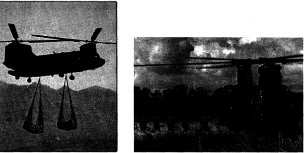
Figure 1.2: CH-47D Chinook Cargo Helicopter ("Chinook Image Gallery", 2006)

1.2 The Defense Aerospace Industry: Post September 11, 2001

With the beginning of the Global War on Terror, the defense aerospace industry underwent a tremendous upheaval. Army helicopters are flying at an operational tempo far in excess of anything previously experienced. During combat

rotations, aircraft are flying as much as four times their peacetime average. These continued deployments have raised four issues that the aerospace

industry was not fully prepared to deal with.

The first adversity involves demand forecasting. For over a decade, defense contractors have compiled a historical database of peacetime part consumption. However, with the armed forces fully engaged in combat operations around the world, this information is no longer valid. The last major military operation occurred during the Persian Gulf War of 1991. This conflict only endured seven months, providing little comparison to the present. With the "War on Terror"

exceeding its fifth year in September 2006, suppliers are struggling to predict the needs of a wartime military. Ultimately, the challenge of accurately forecasting the future parts demand has become even more complicated.

The second issue facing the defense aerospace industry is limited part availability due to increased demand. This occurs for three reasons: battle damage, increased flying, and exposure to harsh environmental conditions.

Battle damaged parts present the most difficult challenge. The reality of warfare creates an unpredictable replacement requirement that includes all parts, at any quantity and in various degrees of repair. The next demand problem arises because aircraft components are reaching their design lifetimes much faster than anticipated. This is a result of both the increased flying and the additional

stresses imposed on the airframe by the combat flight maneuvers employed. A final cause under this topic results from the Army's continued operations in

remote climates. Whether it is the extreme desert heat or elevated mountain altitudes, greater than traditional part failure rates from continuous exposure to environmental conditions are beginning to appear. An example of this is seen in a new type of corrosion damage from ingested sand into rotating components.

Regardless of which cause, numerous components are reaching mandatory retirement much sooner than anticipated, driving demand higher than ever.

The third industry-wide issue is an insufficient supply base. There are an extremely small number of suppliers who are qualified to manufacture

specialized aerospace components. This partially results from the fact that the components are very specialized, the market is small in size and the government imposes strict requirements on suppliers that requires extensive bookkeeping. However, these suppliers are also reluctant to invest large amounts of capital in capacity expansion. The suppliers realize that the fighting will eventually end, and with it the wartime operational tempo that is driving demand. As a result, competing aerospace contractors struggle to have their demands satisfied at suppliers who are already operating at maximum capacity. Unfortunately, these capacity constraints only serve to increase lead times and cost.

The final complexity facing the defense aerospace community is the availability of certain raw materials. Known as the "Berry Amendment," Section 2533a, Title

10 of the United States Code imposes legal obstacles upon defense contractors. The regulation states that certain, "products, components, or materials...must be grown, reprocessed, reused, or produced wholly in the United States if they are

purchased with funds made available to the Department of Defense" (United States, 2006). This list includes certain specialty metals which are essential to military aviation for their high strength-to-weight ratios, corrosion resistance, and thermal properties. Unfortunately, the combination of few domestic suppliers and this procurement restriction often causes lead times for these raw materials to

exceed one year. Additionally, suppliers are forced to purchase these materials at highly-elevated prices. In 2005, the price for titanium, one of the regulated metals, surged over 317% (Toensmeier, 2006). Yet despite this cost, titanium is

a crucial material. In commercial grades, it possesses the same tensile strength as steel, but is approximately half the weight (Kerrebrock, 1992). This regulation

undoubtedly is protecting the jobs of American specialty metal manufacturers; however, it is simultaneously creating waste and inefficiency within every

defense contractor's supply chain.1

1.3 The Corpus Christi Army Depot

Funded and operated by the United States Government, the Corpus Christi Army Depot (CCAD) is one of a few sites dedicated to repairing the 57 end-item

components of the Apache Helicopter and the 119 end-item components of the Chinook Helicopter. An end-item is a major assembly such as transmission, gearbox, pump or hydraulic actuator. Prior to Boeing assuming responsibility for

CCAD's supply chain, the depot was responsible for procuring over 7,000 unique part types required to make the scheduled repairs to the above mentioned end-items. However, because of the previously discussed challenges associated with the current aerospace industry, the government's logistical system was unable to adequately meet the Army's demands. As a result, CCAD reported repair

turnaround times (RTAT) in excess of twice the other repair sites. To solve this problem, CCAD looked to Boeing as the original equipment manufacturer for technical, engineering, and logistical support.

1 The thoughts behind the four industry-wide issues were discussed during numerous conversations with David R. Greenwood (internship supervisor and Boeing Senior Manager in Supplier Management and Procurement for the AH-64 CCAD program). The discussions occurred during June 2006.

In October 2004, Boeing signed a five year, several hundred million dollar

contract to partner with CCAD and assume control of the supply chain that

supports the overhaul and repair program for the AH-64 Apache and CH-47

Chinook. As such, Boeing became the primary vendor to CCAD for all AH-64

and CH-47 repair parts. Boeing was now responsible for establishing and I or maintaining supplier relationships, ordering and purchasing the repair parts and

coordinating for shipment of the parts to the Boeing warehouse at CCAD. At the

warehouse, Boeing employees managed the repair parts inventory, issued the

parts when demanded by the CCAD production cycle and tracked consumption

data. Over the course of the last two years, Boeing has been creating and

refining the CCAD supply chain in an effort to reduce the RTAT and increase the

part availability.

1.4 Creation of the Supply Chain

After award of the contract, Boeing developed a plan for creation of the CCAD support supply chain. The decision was to implement the following phased plan (Thieven, 2004).

Phase 1: Provide technical, engineering, and logistics support services and begin to create bills of material (BOMs) to define the

support material needed. A BOM lists the relationship between an end-item and the parts that are used to construct the end-item. The required quantities of each part are listed on the BOM.

Phase 2: Provide material support for the Apache's 24 and the Chinook's 27 most demanded end-items and open the parts warehouse.

Phase 3: Provide all remaining material support for the non-critical, lower demanded end-items.

Phase 4: Provide material support for airframe structures. This includes modifications for AH-64A to AH-64D transitions as well as repair for battle or crash damage. A transition is an aircraft modernization. An AH-64A model is delivered to the depot by the U.S. Army.

Older technology is replaced with newer versions to increase the helicopter's capabilities. Examples of this include the addition of a target acquisition and identification radar, stronger engines and increased aircraft survivability equipment.

Since establishment of this phased plan, numerous changes have been made to its architecture to include Phases 2a and 2b (expansions of the Phase 2 end-item list). However, the original concept remains the same. At the time of this thesis, Boeing is providing support to CCAD in accordance with Phase 3. Boeing has begun planning for Phase 4 implementation. It should be noted that whenever possible, Boeing has attempted to provide material support regardless of phase assignment.

1.5 Thesis Outline

An introduction was offered in Chapter 1.0. Chapter 2.0 will discuss the current support structure, information and material flow along the supply chain and

highlight the areas targeted for improvement. In Chapter 3.0, the flexibility added

by implementing a fixed pricing strategy is presented. Chapter 4.0 describes

how procurement lead times are reduced by altering the raw material

procurement policy. In Chapter 5.0, a methodology is created for identifying inaccurate Depot Overhaul Factors in order to improve fulfillment rates. Finally, Chapter 6.0 will finish the thesis with conclusions, observations and

2.0

Integration and Understanding

Before recommendations for improvement can be made, it is necessary to understand how the current system operates. How do people communicate? What is working well? What is not? This chapter will address these and other basic questions in an attempt to explain why the areas chosen for improvement were selected.

2.1

Information Flow

Efficient information flow is critical to a well-organized supply chain. The CCAD support structure is no exception to this statement. In order for a repair part to

arrive at CCAD, numerous groups of people must communicate within a

complicated system that spans the entire United States. To manage the thousands of information requirements, Boeing utilizes a centralized database and a material management system known as the Advanced Manufacturing Accounting and Production System (AMAPS). Understanding how people interface with each other and the database will highlight where communication inefficiencies occur and provide insight into where improvements can be made. The figure below attempts to map the information network at a high level. Greater detail will be explored in the following sections.

--- Supplier ---AL4

CCAD Price Quotes tLead Times

• , . .... . .... .

II

Legend

S Information provided to database 4- One-way communication

4- --" Two-way communication Information retrieved from database

Figure 2.1: Communication Network

2.2

How Parts Arrive at CCAD

For parts to arrive at the Boeing Warehouse at CCAD, coordination and planning must be completed prior to the production cycle. Once all of the preparation is completed, the supply chain begins the physical process of ordering and shipping the actual parts to CCAD. This chapter will describe both steps by referring to Figure 2.1.

2.2.1 Initial Processes

Before a single part moves along the supply chain, a support contract is

negotiated between Boeing and the U.S. Government. Of all of the agreements listed in the contract, three of the most commonly referred to are a part's support date, its contract quantity, and its contract price. The support date is the date

that Boeing assumes responsibility for providing a part to CCAD. The support

date is linked to one of the four phases discussed in Chapter 1.4. The contract

quantity refers to the number of parts Boeing promises to provide CCAD once

the support date is reached. This quantity is based upon CCAD's forecasted

production needs. The contract price is a per-unit price Boeing agrees to charge

CCAD for each part. This price is based upon the contract quantity and an

agreed upon profit margin. An example of what this information would look like in the contract is listed below.

Part Number Support Date 2007 Quantity Price

123 01/01/2005 25 $271.68

456 08/31/2007 3 $23.51

789 05/15/2008 0 n/a

Table 2.1: Contract Data Example

Thus, at of the time of this thesis, Boeing would already be supporting Part Number 123. Boeing is required to provide 25 of Part Number 123 during 2007

and will sell each part to CCAD for $271.68.2 Part Number 456 is scheduled to

2 The contract will actually list each part number's requirements for the next three years. Each part number will have a quantity and price associated with the future production year. Prices are adjusted for inflation. Thus, for this example, the actual contract would list quantities and prices for 2007, 2008 and 2009.

be supported on August 31, 2007. Depending on the lead time of the part, Boeing will take the appropriate action to ensure the part is on hand by the

support date. Finally Part 789 is not supported yet. As such, none of these parts are required for the 2007 production year. With the contract completed, parts can be ordered for the upcoming production cycles.

2.2.2 Ordering and Shipping

Each April, the U.S. Army Aviation and Missile Command (AMCOM), provides

Boeing with CCAD's Workload Forecast (WLF). AMCOM is the financial arm that

controls CCAD's budget. The WLF specifically details the number of overhauls

CCAD is funded to repair (per end-item) for the upcoming three years. The WLF

forecast is usually updated with changes on a semiannual basis in October. Quite often, the WLF does not reflect what was listed in the contract quantity.

However, with the WLF on-hand, Boeing can determine the type and number of parts to procure. This begins when the Boeing database pairs the WLF with an estimate for the probability of part replacement. This replacement estimate is required because not every end-item overhaul requires each internal part to be replaced. If an inspection determines that a part is still functional, the part will be cleaned and returned to service. Thus, a factor is used to forecast how many parts will be consumed during each end-item overhaul. This replacement estimate is known as the Depot Overhaul Factor and will be discussed in more

detail in Chapter 2.5. But for now, for each part, the quantity to order can be determined through the following equation.

End-item WLF * Depot Overhaul Factor = Quantity to Order (Equation 2.1)

For each of the 7,000 parts, the database calculates the quantity to order with

Equation 2.1 and transfers the information into AMAPS. Finally, the asset

managers, who are responsible for coordinating with the various suppliers, retrieve the required quantity from AMAPS and work with the Boeing buyers to purchase the parts required to support the WLF.

2.3

Process Timelines

With the flow of information and material mapped, the next step was to gauge the timeliness of the operation. This could provide some insight into where

inefficiencies are creating waste within the supply chain. After talking to the responsible parties, the following functional timeline for actual task completion was developed.

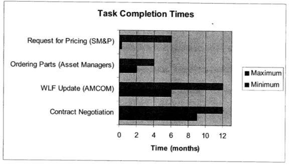
Task Completion Times

* Maximum * Minimum

0 2 4 6 8 10 Time (months)

Figure 2.2: Task Completion Timeline

Two functions are absent from this chart: Depot Overhaul Factor updates and BOM updates. These were excluded because they are continually monitored and sporadically changed. It should also be noted that the WLF update is at the discretion of the U.S. Government and contract negotiations are beyond the scope of this project. Regardless, closer examination of Figure 2.2 reveals some interesting results.

When compared with the other functions, a "Request for Pricing" shows a disproportional gap between the minimum and maximum task completion times. According to SM&P personnel, this disparity occurs when numerous parts require repricing at the same time. Recalling Chapter 2.2.1, when a part is placed on contract, it is priced at a specific quantity. However, as mentioned before,

CCAD's _{WLF will quite often demand quantities that differ from those listed on}

the contract. This volatility in the required quantity affects the price (as a result of

Request for Pricing (SM&P) Ordering Parts (Asset Managers) WLF Update (AMCOM) Contract Negotiation

scale). For example, if CCAD originally contracted for 10 pieces and now requires 100, the per-unit cost to Boeing will be less due to economies of scale.

Thus, the selling price of the part to CCAD will also decrease. Conversely,

decreases in quantities will result in increased procurement costs and selling

prices.

The problem inherent in the fixed contract price is revealed whenever a WLF update arrives. This is because the update encompasses the entire parts list and ranges in scale from -100% to greater than + 100% of the original forecasted requirement. This change in the demanded quantities invalidates the quoted contract price for thousands of parts. In addition, because the price is no longer accurate, Boeing is prohibited from selling the part to the depot. The unfortunate result is that even if the part is on the shelf and available for use by CCAD

personnel, Boeing cannot proceed with the sale. As a result, production must wait while SM&P staff contacts the various suppliers and has new prices

calculated. Figure 2.3 depicts the most recent variability within the CCAD supply

Figure 2.3: Supply Chain Variability in Demand

Figure 2.3 shows magnitude of the change in forecasted demand over a six month period. Only 19% of the 7,000 parts had little to no change in forecast (-5% to +5%). Unfortunately, the remaining 81% of parts experienced significant changes.

While the actual task of submitting a new request for pricing can be completed quickly, suppliers will often take exhaustingly long times to return new quotes. This usually occurs because thousands of parts require repricing at the same time. This delay in acquisition time produces two unfavorable results. First, if an alternate source of supply is available, CCAD will attempt to purchase the part

elsewhere.3 _{Second, if no alternate source of procurement is available,}

3 By contract, CCAD must purchase the parts from Boeing is they are already supported. However, if the required part is not on-hand, CCAD may look to other suppliers for support. Examples of this include other Department of Defense warehouses and other suppliers.

production will stop. Regardless of the result, Boeing loses revenue from the missed sale opportunity and customer satisfaction decreases. This

administrative repricing delay has significant consequences on the production cycle and can be listed as a cause of the less than optimal RTAT. As a result, this is an ideal area for improvement and will be discussed in detail in Chapter 3.0.

2.4 Implications of Variation on Lead times

The supply chain demand variability depicted in Figure 2.3 showed that

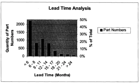
approximately 60% of the part numbers increased in quantity. Unfortunately, the majority of parts that Boeing supplies to CCAD do not possess short lead times. For the purpose of this analysis, a long lead time is defined as greater than or equal to six months. Figure 2.4 shows that approximately 59% of all CCAD parts have long lead times.

Lead Time Analysis 2000 1500 1000 500 0 ,~o o• •'\ L 0 e T Lead Ti 50% 40% _{4 0} Part Numbers 30% _1-o 20% o 10% 0% me (Months)

Figure 2.4: Lead Time Analysis

Additionally, some of the most critical parts to CCAD's production fall on this long lead time list. Critical parts are defined as those required for "flight safety"

purposes, those without which all production will stop or of those significant importance to CCAD and the U.S. Army. Regrettably, many of these critical long lead time items also experience the increased variability seen in Figure 2.3. However, what Figure 2.4 fails to depict is the specific impact of raw material procurement on a part's total lead time. When raw material lead times are examined, only 66 of the approximate 7,000 parts had four similar qualities. These qualities were (1) total lead times in excess of 12 months, (2) a history of the previously described variability in demand, (3) on CCAD's critical demand list and (4) composed of specialty metal raw materials.

a

Recalling Chapter 1.3, specialty metal raw materials are difficult to obtain quickly. When looking at this subset of 66 parts, the average lead time to procure the

required raw materials equates to 62% of an end-item's total lead time. The corresponding range in raw material lead time spans from 31% to 88%. As such, a theory was developed that stated if the raw material for a critical end-item was

available whenever an unforecasted demand was received, the total lead time to produce the end item could be reduced by the raw material procurement time. As a factor of the importance of these parts, Boeing management (with input from CCAD) decided to focus on increasing the fill rate of these 66 parts. An analysis was created to determine if there was a business case to justify

maintaining a safety stock of specialty raw materials for the 66 critical end-items. Furthermore, if the safety stock should be procured, what quantity should be maintained? These questions served as the second area for improvement and will be discussed in detail in Chapter 4.0.

2.5 The Depot Overhaul Factor

Briefly mentioned in Chapter 2.2.2, the Depot Overhaul Factor (DOF) is an average component part failure rate that Boeing uses to help forecast the future parts demand. For every part on each end-item, Boeing determined a DOF. Boeing defines the DOF as the quantity of a specific part consumed per 100 overhauls. It is important to stress that a DOF is unique to each end-item. Thus, a part will have a DOF for every end-item in which it appears. However, if a part

is used in various locations within a single end-item, the assigned DOF will be common to the part regardless of how it is used (Wart, 2006).

For example, "Gear XYZ" is utilized within two end-items: the fuel transfer valve and the auxiliary power unit (APU) shut-off valve. Within the fuel transfer valve,

"Gear XYZ" has a DOF of three, while in the APU shut-off valve; it has a DOF of

five. Thus, on average, Boeing anticipates having to replace "Gear XYZ" three out of 100 times in the first case and five out of 100 times in the latter. Utilizing

Equation 2.1, if the WLF for the fuel transfer valve is 200 and there is only one "Gear XYZ" per valve, Boeing will order six gears in anticipation of the production year.

The DOF selection is based upon input from a variety of sources. These sources include (but are not limited to) CCAD historical records, engineering

specifications, human input and other program recommendations. Unfortunately,

the various sources rarely agree upon what the DOF should be. As such, a

prioritization scheme was established to choose the appropriate DOF. However, these disagreements have recently caused Boeing management to question the

accuracy of the DOF list. As a result, an analysis was created to determine the

appropriate selection criteria and usage of the DOF. The third and final aspect of this thesis evolved from this analysis. With a database of thousands of DOF values, a methodology would need to be created to highlight potential focus

areas. This methodology along with the associated problems and limitations of the current DOF usage will be discussed in Chapter 5.0.

3.0 Exploring Fixed Unit Pricing

Whenever possible, Boeing and AMCOM personnel will meet face-to-face to discuss issues affecting the operation of the CCAD supply chain. During these coordination meetings, new ideas are proposed in attempts to improve upon any identified problems. In July 2006, one of these meetings took place where an idea was suggested to address the timing problem caused by an updated

forecast and the need to reprice parts. The idea was to fix the contract sale price of a part as a constant, regardless of the quantity ordered. In other words, once the part was priced for a certain quantity, the quoted contract value would remain

the selling price regardless of what quantity was sold to CCAD.4 _{Recalling Table}

2.1, Part 123 was priced at $271.68 for a quantity of 25. Under this plan, the $271.68 selling price would apply if CCAD only ordered 11 or 1100.

This idea, which became known as the "fixed pricing" solution, would mitigate the effects of the government's poor and variable forecast by eliminating the need to obtain a new price quote. Without the repricing delay, a part could be sold upon request and the supply chain could eliminate inefficient delays. However, fixed pricing would require Boeing to assume two types of risk from the downside of this pricing solution. These risks are discussed in the following chapters and are the starting point for an analysis to determine if the fixed pricing idea is an acceptable solution.

3.1

Risk Due to Quantity Fluctuation

The first hazard with fixed unit pricing is classified as risk due to quantity fluctuation. As discussed earlier, contract prices are based upon a specific quantity. Assuming economies of scale hold true, the more parts ordered, the smaller the per-unit cost. This affect occurs because the fixed costs of

production are now dispersed over an increasing number of units. The quantity fluctuation risk becomes relevant when Boeing prices a part for one quantity and

CCAD orders significantly less. Figure 3.1 below depicts an example of this

issue.

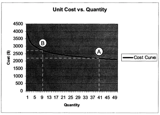
Unit Cost vs. Quantity

4500 4000 3500 3000 S2500 o 2000 1500 1000 500 0 -Cost Curve 1 5 9 13 17 21 25 29 33 37 41 45 49 Quantity

Assume the contract price is represented by Point "A." Here, a quantity of 40

parts equals a cost of $2200 per unit. However, if CCAD alters their demand to

Point "B," the new quantity of ten parts has a higher unit cost of $2700. For this example, a fixed price agreement will cause Boeing to lose $500 per part.

3.2

Risk Due to Material Escalation

The second type of risk generally results from raw material costs. As mentioned during the industry overview, certain specialty metals have tripled in price over the last year. Without long-term price agreements with suppliers, material escalation costs would likely be transferred onto Boeing. Once again, Boeing would lose money in a fixed price scenario as they would be unable to transfer

these additional costs onto CCAD.

As an example, refer again to Part 123's contract quantity and price of 25 and $271.68 (from Table 2.1), respectively. Assume that Part 123 is built entirely from Titanium. If Titanium prices rise another 317% as in 2005, Part 123's

supplier will undoubtedly pass this additional cost onto Boeing. This would result in a new unit cost of $861.23. Fixed unit pricing would require that Boeing lose $589.55 per unit because they would still be forced to sell the part at the original cost of $271.68.

3.3 Data Gathering

With an understanding of the risks involved, the research into fixed pricing could begin. Responsible parties from the following functional groups involved in a repricing assignment were interviewed: supplier management and procurement (SM&P), asset managers and contracting personnel. It was during a discussion with the asset managers that the first piece of information critical to the analysis was found.

3.3.1 Discussions with the Asset Mangers

Recalling Chapter 2.2.2, asset managers are tasked to supervise and administer Boeing's requirements with key suppliers. Specifically, asset managers

coordinate with suppliers to ensure that the requested parts arrive at CCAD to support the production schedule. However, what Boeing failed to capitalize on was that the asset managers also oversaw the parts flow to other assembly and repair programs. Some of these other accounts include the production line, aftermarket part sales direct to the military and other overhaul and repair programs.

The asset managers would determine and load the purchase requirements for the different programs separately. In turn, the buyers would react to these requirements as they were loaded, by placing individual purchase orders. This effectively eliminated the benefits of scale. As all of these parts support the military, they are funded in the same fiscal year. Thus, the demand and

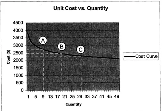
financing for these parts are known and available at the same time. There was nothing preventing the asset managers from combining the demand, placing one total order, leveraging economies of scale and achieving cost savings. A revision of Figure 3.1 demonstrates this.

Figure 3.2: Leveraging Economies of Scale

If an asset manager purchases parts for Program A and Program B separately,

he would pay $2750 and $2500 per unit, respectively. However, if the asset manager combines the two program's demands and places a single order (represented by Point C), the per-unit cost is now $2250. Thus, the power of economies of scale is revealed.

Unit Cost vs. Quantity

4500 4000 3500 3000 S2500 o 2000 1500 1000 500 0 --- Cost Curve 1 5 9 13 17 21 25 29 33 37 41 45 49 Quantity

3.3.2 Non-CCAD Demand for Parts

The next step was to determine the historical parts demand for programs other than CCAD from 2003 through 2006. These years were selected because they isolate the wartime demand. For all the parts that support CCAD, the yearly demand for all the other programs was gathered. The data revealed that these programs were different from CCAD in that when orders were placed, the quantities rarely changed from the original forecast. These programs were not experiencing the fluctuations in demand that CCAD was. Additionally, the other programs provided significant demand (in terms of quantity) to justify exploration into the benefits of economies of scale. This evidence provided the second key to the fixed pricing analysis.

3.4 Data Analysis

In order to support CCAD with repair parts for both the AH-64 and CH-47, Boeing must manage 7,000 unique part numbers. To make this list more manageable and meet an October 2006 implementation goal, a subset of part numbers were chosen for the analysis. Only parts that had an active support date and

possessed a unit price greater than $100 would be included. The $100 unit cost cutoff was chosen for three reasons. First, Boeing purchases most parts under

$100 in bulk for a four year contract requirement. Second these parts represent

approximately 70% of the total part list. By purchasing these parts all at once, numerous transactions can be eliminated and time can be saved. Finally, parts less than $100 equate to only 5% of Boeing's total cost. This safety stock of

inventory increases fill rates at a minimal cost. By looking at the active support dates and unit costs greater than $100, the resulting subset equaled 1,793 part numbers and represented 94% of the contract's total revenue.

3.4.1 Risk Mitigation from Quantity Fluctuations

A part is protected against the risk from quantity fluctuation if its cost to Boeing can not increase. Another way of stating this is that if a part is on contract for a small quantity, it can be assumed that the cost to Boeing is already at its

maximum. This is true because of a practice commonly employed by Boeing's suppliers. Known as quantity band pricing, a single price is applied to a range of quantities in order to save time. These bands vary in quantity; however, the first tier is frequently from the first unit to the tenth. Thus, the price of the first item is the same as the price of the tenth.

In order to save time, suppliers will often limit their quantity band pricing to the vicinity of the submitted contract quantity. Thus, for Part 123 from Table 2.1, the

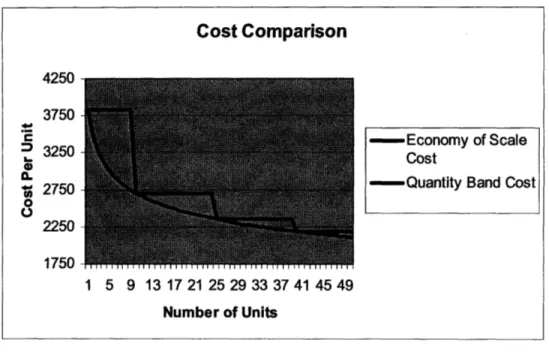
price of $271.68 might apply for quantities 21 - 30 where a price of $250 might apply to a range of 31 - 50. Figure 3.3 depicts this assumption by overlaying typical quantity band pricing onto the cost curve from Figure 3.1. The bands are

applied across the entire cost curve to better illustrate the example. The figure shows how the benefits of scale still exist, but not incrementally.

Cost Comparison

Figure 3.3: Cost Comparison

In looking solely at the economy of scale cost curve, quantity decreases where

the slope is steepest would have an enormous impact on the cost of an item. However, in quantity band pricing, a decrease in quantity from nine to three (for example) has no impact on cost to Boeing. This concept was applied to the subset of part numbers in the fixed pricing analysis. As discussed above, the assumption used was that contract quantities less than 10 were already priced at their highest cost to Boeing. Figure 3.4 shows the results.

4ZDU 3750 S3250 S2750 0 2250 1750 -Economy of Scale Cost

- Quantity Band Cost

1 5 9 13172125293337414549 Number of Units

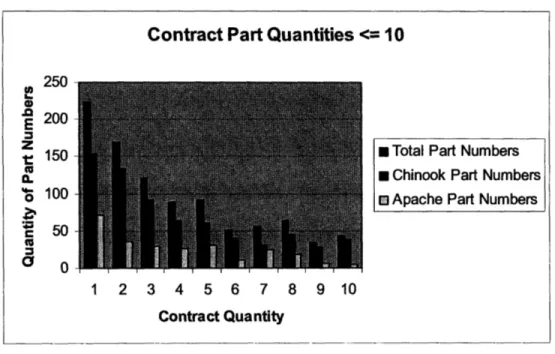
Contract Part Quantities <= 10 250 S200 z S150 0. 0 100 50 U0

n Total Part Numbers

m Chinook Part Numbers

E Apache Part Numbers

Figure 3.4: Small Contract Quantities

These 945 part numbers represent 9% of the total contract revenue and 53% of the subset of parts. Because these part numbers are on-contract for small

quantities, there is little risk associated with fixed pricing. Combined with the small amount of revenue represented, quantity decreases for these 945 part numbers will have minimal to zero effect to Boeing.

3.4.2 Revenue Implications of Fixed Unit Pricing

With 53% of the part numbers essentially protected from quantity fluctuations, the question turned to how will the selected parts influence revenue under fixed unit pricing. The 1,793 parts were examined using three filters: revenue potential, contract quantity, and percentage of demand. Revenue potential represents the amount each part number is expected to earn if the entire contract quantity is sold. For example, if a part number's contract quantity is 10 and the contract

12 3 4 5 6 7 8 9 10 Contract Quantity

price is $100, the revenue potential is equal to $1000. Contract quantity was already discussed in Chapter 2.2.1. Demand percentage evaluates how much of a part number's total demand belongs to CCAD and how much belongs to the other assembly and repair programs. Two assumptions were used in this portion of the analysis.

1. Part numbers with contract quantities greater than 10 represent an increased risk for fixed pricing and the possibility to incur higher costs. This is because quantities greater than 10 are outside of the minimum

quantity band price range.

2. If CCAD's share of a part number's total demand across all programs is greater than 50%, the part number is exposed to increased risk from quantity fluctuations and higher costs. This was based on the information discussed in Chapter 3.3.2.

Figure 3.5 below depicts the results of this analysis. It should be noted that the quantities represented under each revenue column are inclusive and represent a minimum level of revenue potential. Thus, a part number included under the

$1M column is also included in the $750k, $500k, $250k and $100k potential

Contract Revenue Sensitivity

Figure 3.5: Contract Revenue Sensitivity

This figure displays categories of high revenue earning part numbers that have the potential to vary greatly in quantity. For example, there are 88 part numbers with a revenue potential of $250k. Of those 88 part numbers, 83 are on-contract for a quantity greater then 10. This implies that if there is a decrease in the

quantity required by CCAD, Boeing would incur additional costs under a fixed

unit pricing strategy. Of those 83 part numbers, 69 have greater than 50% of

their total demand satisfied by CCAD. This implies that the majority of demand is

subject to the quantity fluctuation risk. This again indicates risk to Boeing under fixed unit pricing. The shaded columns represent a request from Boeing

management for financial implications. (i.e., the 83 part numbers that have a revenue potential of $250k and are on-contract for quantities greater than 10

250 S • 200 E z S150 0. 4 0100 S50 a 0 $100k $250k $500k $750k $1 M

Contract Revenue Potential

* Revenue Earning Part Nurrbers

* Contract Qty > 10

o Qty and CCAD Demand >

equate to 56% of the total contract revenue). As a result, the represented part numbers are good candidates for removal from fixed pricing.

3.4.3 Recommended Exclusion List

Based upon guidance from Boeing management, a decision was made to expand the revenue implication analysis, but only include revenue potential and contract quantity. The CCAD demand filter was removed and the following results were found.

Potential Revenue and Contract Quantities > 10

70% t'-0.

Ez

Potential Revenue (thousands)

$170 115 106 61% $180 109 103 60% $190 108 103 60% $200 105 100 60% $210 99 94 59% $220 97 92 58% $230 91 86 57% $240 89 84 57% $250 88 83 56%

Figure 3.6: Exclusion List Recommendation

250

The table expands on the previous chart with the shaded cell representing the recommendation to management for exclusion from fixed unit pricing. The 100 part numbers each have a potential contract revenue of $200k or greater and are on contract for quantities greater than 10. By removing the associated 100 part numbers, Boeing protects 60% of the contract's revenue potential from the risk due to quantity fluctuation. As a footnote, management subsequently added an additional 54 part numbers to the exclusion list due to high susceptibility for material escalation risk. The 54 part numbers were linked to suppliers who would not agree to long-term pricing agreements for protection against raw material cost escalation.

With the 154 part exclusion list finalized, 7,044 parts would no longer need repricing from changes in forecasts. However, before agreeing to the fixed

pricing strategy, Boeing requested the construction of a Monte Carlo simulation to determine the impact on income from sales due to the effects of fixed pricing on the 7,044 parts.

3.5 Monte Carlo Simulation

A Monte Carlo simulation is a stochastic technique which randomly chooses

values for uncertain variables in order to estimate the probability of various outcomes. Crystal Ball software (version 7.2.2) was used to construct the fixed unit pricing simulation. The Crystal Ball software is a Microsoft® Excel-based application distributed by Decisioneering, Inc for risk analysis and optimization

studies. The "high-level" flow diagram in Figure 3.7 will be referenced to explain the architecture, assumptions, calculations, and processes employed in the

Monte Carlo simulation. Finally, the results from the simulation and from the actual implementation will be discussed.

End IternWLF

---I

K

7

I I

Markup

Rate ContractPrice

kicomne Comparison

then Reilerate

Legend

[=3

0

Figure 3.7: Fixed Unit Pricing Monte Carlo Process Flow Chart

3.5.1 Monte Carlo Data

Input

Construction of the model began with the input of the following data:

1. 176 end-items for both the AH-64 and CH-47. 2. WLF for each end-item.

3. 1,693 subset part numbers associated with the end-items (The 100 recommended exclusion parts were removed from the simulation. The 54 additional parts removed from fixed pricing were already filtered out by my initial screening of the 7,000 parts).

4. CCAD WLF for each part.

5. Non-CCAD annual demand (four-year historical average from 2003 through 2006) for each part.

6. Contract price associated with each part. 7. Contract quantity for each part.

This WLF data used was based upon 2007 requirements only. Additionally, if a

part was priced on either Phase IIA or Phase Ill contracts, the higher price was

utilized.

3.5.2 Assumptions

The first assumption made during the construction of the Monte Carlo Simulation was how to replicate the variability within the WLF. Unfortunately, historical variability within each end-item's WLF was not maintained past the previous six-month update. Thus, a customized distribution could not be constructed.

the WLF (depicted in Figure 2.3) were typical of historical trends. As a result, the decision to use a Beta - Program Evaluation Review Technique (PERT)

distribution was chosen.

The PERT manipulates the beta distribution and is similar to the commonly known triangle distribution in that a minimum, mode, and maximum value are known. However, the PERT distribution deemphasizes the minimum and maximum values by replicating the distribution with a smooth curve. This prevents skewing the results towards the extreme ends of the distribution. The PERT also converts the mean of the distribution to be the average of the

minimum, maximum, and four times the mode. This once again removes the bias of the distribution's tails and is a commonly used technique for procurement studies (Roman, 1962).

As the current trend for variability within the WLF favors an increased demand, the following parameters were chosen to generate the PERT distribution.

1. Minimum: -50% of the WLF

2. Mode: WLF

3. Maximum: +100% of the WLF

By comparing a revised Figure 2.3 with a PERT distribution graph generated by the Crystal Ball software, a visual resemblance can be observed.

Variability in Demand

(Without -51% and Less)

1600 1400 1200 1000 800 600 400 200 0 M Part Numbers -Poly. (Part Numbers

Figure 3.8: PERT Distribution

Replicating Quantity Band Costs

Over the course of each trial, the Monte Carlo simulation has the potential to demand any quantity within the -50% to +100% distribution. However, quantity

band costs were not available for each part. Additionally, inputting 1,693 quantity band values would have been extremely time-consuming. As such, the

assumption was made to use a 90% log-linear experience curve to replicate the

cost of each part at any quantity. Essentially, every time a part's quantity

doubles, the cost of the part decreases by 10%. Argote, et al explain how within industrial settings, an 80% experience curve is commonly observed as processes are repeated (1990). However, a 90% curve was chosen to find a more

conservative solution.5 _{The equation used to construct the curve is listed below}

("Cost Estimating," 2006).

5 The 90% cost / quantity curve is commonly used within the aerospace industry and is generally accepted by the U.S. Government and their audit agency (the Defense Contract Audit Agency) as a reasonable curve for determining cost with changing quantities.

4)

Y = CI * Xb (Equation 3.1)

Y = Cost of unit

C, = Theoretical cost of first unit

X = Number of unit produced b = In(90%) / In(2)

The curve was developed by using the only known cost information: a part's contract quantity and its associated price. Since the contract price is what

Boeing charges CCAD, the original cost was calculated by removing the standard markup rate. For example, part "ABC" is listed on the contract at a quantity of 20 and a unit price of $500. Assuming the standard markup rate is

10%, the cost of each part would equal $454.55 when 20 are ordered. This information could then be substituted into the Equation 3.1 to construct a cost for each trial's quantity.

While cost reduction through learning and cost reduction through quantity discount purchasing occur for two separate reasons, an experience curve "reflects the joint effects of learning, technological advances and scale" (Reis,

1991). To validate this assumption, a comparison from known quantity band cost tables and the assumed experience curve was developed. The resulting figures for two sample parts are listed below.

Part "ABC"

Figure 3.9: Experience Curve vs. Quantity Band Costs

The curves closely follow the quantity bands. However, there is a difference in the magnitude of the costs. This can be explained by looking at the time frame from which the data originated. The experience curve is based upon cost

estimates for 2007 using 2006 data. The quantity band curve is an estimate of

2007 costs from 2005 data. These changes in cost estimates could arise for

numerous reasons to include raw material escalation or increased labor costs at the supplier. Regardless of the reason, the 90% curve follows the quantity band's trend and is a reasonable approximation for cost.

3.5.3 Trial's Calculations and Process Flow

With the data collected and the assumptions made, the model was constructed. Every time a trial is run, the model alters CCAD's original end-item WLF by a random draw from the PERT distribution. All of the parts within each end-item are changed accordingly and summed with the CCAD demand. The

non-CCAD demand never fluctuates as it represents demands which experience little

to no volatility. An example of these steps can be seen by using "Gearbox ABC"

1400 1200 1000 S800 600 400 200 0 1-90% Curve PY2006 60-Quantity Band WLF2A5-17-05 1 14 27 40 53 66 79 92 Quantity

below. Three notional parts (001, 002 and 003) are used to build "Gearbox ABC."

Gearbox "ABC" Original WLF 100

Trial Variation 1.2

Gearbox "ABC" Trial WLF 120

€ -1. PERT distribution varies demand.

Part Number CCAD Original Demand CCAD Trial Demand Non-CCAD Demand Total Trial Demand

001 8 10 19 29

002 10 12 34 46

003 37 45 41 86

2. CCAD part demand is varied equally. 3. CCAD Trial + NON-CCAD = Total

Figure 3.10: Demand Calculations

With the total demand for the trial known, the cost for procuring each part will be calculated with the experience curve described in Chapter 3.5.2. This cost is then used to determine the income from sales under both fixed pricing and the traditional method of using a standard 10% markup rate. While the total demand from the CCAD and the Non-CCAD programs is used to calculate the trial's scaled cost, only the income from the sale of the CCAD demand is recorded.

The equations used and the example from Figure 3.10 are continued below. 6

Fixed Pricing Income = CCAD Demand * (Contract Price - Scaled Cost)

Markup Income = CCAD Demand * [(Markup % * Scaled Cost) - Scaled Cost]

(Equation 3.2) (Equation 3.3)

6 The contract quantity and price would be retrieved from the contract. The contract cost was calculated by removing the 10% markup rate.

Part Number Contract Quantit Contract Price Contract Cost

001 8 $ 1,000.00 $ 909.09

002 10 $ 100.00 $ 90.91

003 37 $ 500.00 $ 454.55

Part Number Total Demand Scaled Cost CCAD Demand Fixed Price Income MarkupIncome

001 29 $ 747.46 10 $ 2,525.35 $ 747.46

002 46 $ 72.09 12 $ 334.94 $ 86.51

003 86 $ 399.85 45 $ 4,506.67 $ 1,799.33

Example with Part 001: Using Equation 3.1:

Using Equation 3.2: Using Equation 3.3:

C, = e[LN($909.0 9)-(LN(90%)/LN(2))*(LN(8))] = $1,247.03 Scaled Cost = $1,2 4 7.0 3*2 9(LN(90%)/LN(2)) = $747.46

Fixed Price Income = (10) * ($1000 - $747.46) = $2,525.40

Markup Income = (10) * [(1.1 * $747.46) - $747.46] = $747.46

Figure 3.11: Cost and Income from Sales Calculations

For the example with Part 001, the fixed pricing method would yield $1,777.94 more in income from sales than the traditional markup method. However, this financial increase is a result of both increased sales volume (two units) and lower

costs. Nonetheless, if the CCAD demand does not increase, but is held constant at eight units while a scaled cost of 27 units (from the total demand) is calculated, an increase in income from sales of $1,350.47 can still be achieved. This shows the cost saving benefits derived from economies of scale.

3.5.4 Simulation Results

We ran the Monte Carlo simulation for 10,000 trials. After each trial, the simulation recorded the difference between the fixed price income and the

standard markup income. At the conclusion of the simulation, the fixed price income resulted in a mean increase of 11% over the standard markup income. A histogram from the simulation's outcomes is presented below. The actual values have been replaced with percentages for proprietary reasons.

Figure 3.12: Monte Carlo Simulation Results

The rise in the income from sales is dependant upon each end-item's ability to increase to +100% of the original WLF. However, even if all of the end-items were to simultaneously fall to -50% of their WLF, the income from sales would still increase by 3%. Although statistically improbable, this event displays the

true benefit of cost reductions and the value of summing the demands from all

repair and overhaul programs.

Aside from the increase in income, the fixed pricing methodology provides

considerable advantages. Foremost, the repricing delay caused by the variations in demand will be eliminated except for the 154 excluded parts. Recalling Figure

2.2, this can potentially remove six months from the procurement cycle.

Assuming the part is on-hand, a sale will occur as soon as the request is made. This will also simplify the maintenance of the contract when CCAD requests parts over-and-above the previously agreed upon quantity. Additionally, customer satisfaction will increase due to the improved responsiveness. The increased flexibility will have a positive impact on CCAD's repair turnaround times since unforecasted parts will arrive much sooner. This will also decrease the holding costs associated with keeping inventory on the warehouse shelves. Finally,

Boeing will stop losing sales to alternate sources of supply, further increasing its revenue.