CHANGING HOUSEHOLD STRUCTURE AND
THE IMPACT ON THE JOURNEY TO WORK
by
Malcolm Morris Quint University of Massachusetts
(1982)
SUBMITTED IN PARTIAL FULFILLMENT OF THE REQUIREMENTS OF THE
DEGREE OF MASTER OF SCIENCE
IN TRANSPORTATION
at the
MASSACHUSETTS INSTITUTE OF TECHNOLOGY June 1985
Q Malcolm M. Quint
Signature of Author / '
Department of Urban Studies and Planning
Certified by
Moshe Ben-Akiva Thesis Supervisor Accepted by
Amedeo Odoni Chairman, Master of Science in Transportation Committee
ABSTRACT
CHANGING HOUSEHOLD STRUCTURE AND
THE IMPACT ON THE JOURNEY TO WORK
by
MALCOLM MORRIS QUINT
Submitted to the Department of Urban Studies and Planning on May 17, 1985 in partial fulfillment of the
requirements for the Degree of Master of Science in Transportation
The trends in household structure were examined to determine their relationship to residential location. Knowledge of the
residential density in an urban area is a key component in planning transportation capacity, especially for the demand during commuting
hours. The married couple category accounts for the majority of
households though single member and single parent households have the
highest rate of growth. The motivation for this study was to examine whether the wider diversity in the living arrangements of Americans
has affected the patterns of residential density in metropolitan
areas. An objective was to determine the significance of household structure in the choice of housing attributes and its location. Economic theories of residential location assume the presence of one dominant type of household. If this assumption is invalid then models which forecast residential density and travel demand should reflect the diversity of household types.
A regression analysis of housing choices was performed using 1980
Census data on the Boston metropolitan area. The relationship of household structure with housing attributes, commuting travel times, and status of the residential area was modelled. Household structure categories have explanatory power in predicting choice of housing
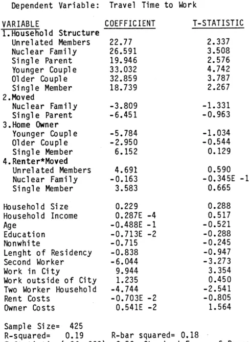
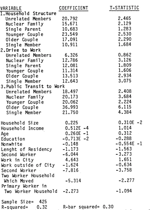
attributes. These categories were less useful in forecasting residential location. Household structure is not correlated with travel time to work. Number of workers in a household is a
significant variable in predicting travel time. The type of household structure is related to the members' preferences in housing.
Thesis Supervisor: Dr. Moshe Ben-Akiva
ACKNOWLEDGEMENTS
I wish to acknowledge the guidance and support of my thesis
advisor, Moshe Ben-Akiva. I, also, want to thank my academic advisor, Ralph Gakenheimer and the head of the department, Nigel Wilson for their assistance.
While this thesis was done as independent research, it was not carried out in isolation. I appreciate and wish to acknowledge the
support provided by my friends, especially Mary, and fellow office mates. The group of students who work the midnight shift in the
Transportation Computer Lab deserve special mention.
I dedicate this thesis to my parents, Donald and Bernice, who have given me their knowledge on the value of the family. This work was made possible by their unwavering support.
TABLE OF CONTENTS
Chapter I: Introduction ... 6
Chapter II: Economic Theories of Residential Location 2.1 Introduction ... 11
2.1.1 Assumptions on Household Strucuture ... 12
2.2 Origins of the Theory ... 13
2.2.1 Land Economics ... 14
2.2.2 Human Ecology ... 15
2.3 The Urban Economicists ... 16
2.3.1 Alonso's Theory of Residential Location .. 17
2.3.2 Muth's Model of Residential Location ... 19
2.3.3 Comparisons of Alonso's and Muth's Models. 20 2.4 Kain and the Journey to Work Model ... 21
2.4.1 Effects of Household Structure ... 23
2.4.2 Causes for Suburban Migration ... 24
2.4.3 Summary of the Contributions by Kain ... 25
2.5 Exodus to the Suburbs ... 25
2.5.1 Relevance of Household Structure ... 27
2.5.2 The Follain and Malpezzi Study ... 27
2.5.3 Grubb's Emplyment Location Study ... 28
2.5.4 Location of Upper Class Residence ... 29
2.5.5 Impact of Transportation Technology ... 30
2.6 Conclusions ... 32
Chapter III: Demographics and Household Structure 3.1 Introduction ...
3.1.1 Five Basic Trends ... 3.1.2 Impact on Urban Planning ... 3.1.3 Causal Relations of Trends ... 3.2 Household Size ...
3.2.1 Household Formation Trends ... 3.2.2 Rise of the Non-Family Household 3.2.3 Decline of Household Size ... 3.3 Trends in Fertility ...
3.3.1 Long Term Cycles of Fertility .. 3.3.2 Theories of Fertility Cycles ... 3.3.3 Effects on Age Structure of the 3.4 Women and Work ...
Population 3.4.1 Married Women in the Labor Force ...
34 35 36 37 38 39 39 43 45 46 46 49 51 52
3.5 The Changing Nature of Conjugal Relations .... 54
3.5.1 Divorce Rates ... 55
3.5.2 Contraceptives and Sexuality ... 55
3.5.3 Social Attitudes toward Divorce ... 56
3.5.4 Economic Independence of the Wife ... 57
3.5.5 Divorce Rates Stabilize ... 58
3.5.6 Remarriage Rates ... 59
3.5.7 Single Parents ... 59
3.6 Conclusions ... 61
3.6.1 Predictions on Household Composition ... 61
Chapter IV: Relationship of Household Structure and Residential Location 4.1 Hypotheses on Impact of Household Structure 65 4.2 Hypotheses on Future Preferences for Residential Location ... 66
4.3 Impact of Demographic Trends on Residential Location ... 66
4.4 Methods of Examining the Relationship of Household Structure to Residential Location 69 4.5 Impact of Other Factors ... 72
Chapter V: Empirical Analysis 5.1 The Data Set ... 77
5.2 Approach to Empirical Analysis ... 78
5.3 Dependent Variables ... 79
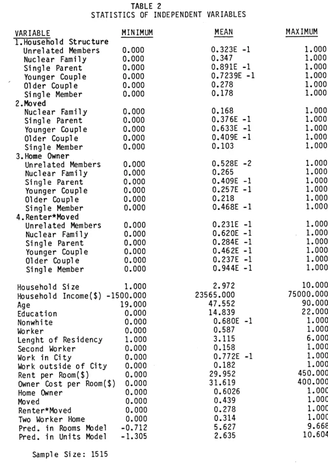
5.4 Independent Variables ... 82
5.5 Estimation Results ... 85
5.5.1 The Relocation Model ... 85
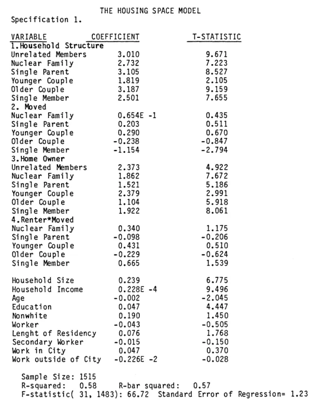
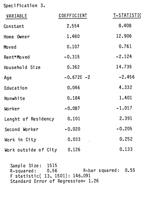
5.5.2 The Housing Space Model ... 87
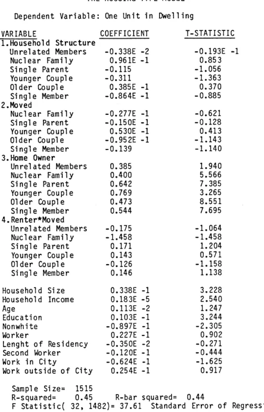
5.5.3 The Housing Type Model ... 91
5.5.4 Travel Time to Work Model ... 96
5.5.5 Class of Residential Location Model ... 100
5.6 Summary ... 107
Chapter VI: Conclusions ... 108
Tables ... 113
TABLES
Statistics of Dependent Variables
Table 1 ... 113 Statistics of Independent Variables
Table 2 ... 114
Explanation of Variables with a Table 3 ...
The Relocation Model Table 4 ... Range of Values .... 116 .. . . . .. . . . . 117 The Housing Table 5.1 Table 5.2 Table 5.3 The Housing Table 6.1 Table Table Table Space Model Type...l ... ... Type Model 6.2 6.3 6.4 ... 118 ... 119 .... 120 .121 .122 .123 .124 Travel Time Table 7.1 Table 7.2 Model ... 0 0 ... 0 * .. . . . .. . . . 125 .. . . . .. . . . 126 County Group Communities by Class
Table 8
Status of Residential Location Model Table 9.1 ...
Table 9.2 ... Table 9.3 ... Table 9.4 ...
Household Structure Groups and Status Location Table 10.1 ... Table 10.2 ... Table 10.3 ... .127 ... 128 ... 129 ... 130 ... 131 of Residential ... 132 ... 132 ... 133 ..
0
.. . .. 0 .. . .. 0 .. . ... 0 0 ... * 0 ... 0 0 ... 0 0 . . . . ... 0I. INTRODUCTION
Human societies are continuously evolving. From the vantage point of one individual lifetime a particular change might seem very dramatic yet over the course of several centuries the change may have
had a minimal impact. The family is a basic component of society which we use as a point of reference. The definitions used to
describe the family have changed over time. The role of the family in Anerica has changed during the course of our history (Skolnick and
Skolnick,1983). Since the second World War the trends in the composition of the family have fluctuated dramatically (Masnick and
Bane,1980). Are the current changes in family structure temporary aberrations or is a fundamental shift occurring in a basic component
of society?
The city planner is always concerned with major trends which affect society. Does the urban master plan, designed in the past, suit the future needs of the area's residents? Knowledge of the fundamental trends in society is imperative if we are to design for the demands of tomorrow. To know when a transportation investment is prudent requires information on the level of demand that service is
likely to generate. Predicting future demand requires the planner to understand how people determine their needs. The choices citizens
make are affected by the composition of their household. A young adult, living alone has different priorities in her demand for transport services than a single mother with two children.
A basic element of transportation planning is the forecast of travel patterns in a defined area. One basic component of this
analysis is predicting where people live and where they work. Simply knowing the percentages of the locations of work and home will not reveal the travel pattern over the transportation network. To design
for system capacity during the peak hours of the work commute, the planner must have information on the expected loads over the major links of the network. To plan for future capacity we must anticipate the location of tomorrow's residences and employment sites. This
thesis examines the relationship of residential location to the changing structure of households.
Predicting the course of current trends is a tricky task. Was it possible to anticipate the baby boom in America after the second World War? Could planners be expected to forecast the rapid growth in suburban residences? Examining these trends with hindsight makes these phenomenon appear almost inevitable. For fifteen years family formation had been slowed by economic depression and then war. Much of the population was employed during the war years but purchases were constrained by rationing and shortages, leaving a large pool of
savings. These elements helped to create the post war boom in high rates of feritility (Fuchs,1983) and increased consumer spending. Such a neat picture of the past does not do justice to the complexity of forecasting such trends before they occur. At the conclusion of
this War many economic forecasts expected a long period of
readjustment before industry would be geared for civilian products. Can we accurately anticipate the unknown future which appears so certain when examined as history?
Many of the trends shaping household structure in today's society will affect the pattern of residential location. Care must be taken before predicting these future patterns from the relationships which existed in the past. Many of the changes in household structure suggest an increase in urbanization. The increase in single member households and in the population over sixty-five years of age signals
rising demand for residence close to services found in the city. But while household patterns are changing so is the structure of
metropolitan areas. Services, once found only near the urban core have been relocating to suburban areas. Employment is no longer centered in the downtown area of a metropolitan area (Grubb,1982). While the priorities of households may be shifting so is the location of the services these households are seeking. The interactive effects between supply and demand over time must be examined closely before predicting future travel patterns.
Given the many layers of changing elements affecting travel behavior, finding the core of the pattern appear impenetrable. To develop theories which serve as tools for anticipating future needs,
simplification of these patterns is required. Constructing models to mirror the key components of the trends is one technique. The ever
present challenge is to simplify the task by including the essential elements and pare away the distraction of superfluous ones. This
thesis examines one component, residential location, which has a major influence on the demands placed upon the transportation network.
Household structure is examined to understand it's impact on the
choice of residential location and determine if it is a key component.
The thesis has four main components. The next chapter reviews the theory of residential location, primarily as studied in the field of urban economics. The relationship between household structure and residential location is revealed in many of the theories of urban economics. In general, economists have taken the structure of the family as a given and not probed the changes occurring to it. The third chapter examines the nature of the changes occurring within the
American family. It addresses whether these changes are fundamental or temporary in nature. The fourth chapter examines the impact different household structures have on the choice of housing
attributes and location. The fifth chapter undertakes a modelling exercise of residential location and travel patterns in the Boston Standard Metropolitan Statistical Area. The final chapter draws
II. ECONOMIC THEORIES OF RESIDENTIAL LOCATION
2.1 Introduction
Urban economics has developed as a separate branch of economics only in the past twenty-five years. In this period economists have
developed theories on the underlying forces of urban spatial
development. Among the various phenomenon they have studied is the relationship between residential and employment locations.
Through research of urban spatial patterns, economists have developed theories of urban growth. One useful concept in their efforts is the bid rent curve (e.g. Alonso,1964). The theory behind this concept is that the value of land is determined by the bid price set by potential users of the resource. Land which is close to the center of a city has a high bid price due to the advantages of
accessibility. Thus the bid rent curve should be downward sloping as distance increases from the center of the city. From this concept the idea of rent gradients was developed (e.g. Muth,1969). The bid rent curve will not be a smoothly shaped inverted cone with the center in the middle of the city. Peaks and valleys will develop around nodal points in an urban area. In essence, a city can be mapped like a mountain range, using the value of land instead of height from sea
level to determine contour lines. Such a map would give a clear indication of the rent gradient for that locale.
From these concepts of land rents, came theories of spatial development. Certain types of businesses will locate in the city
center because they require the maximum accessibility to various markets. Residential areas will be pushed away from the center.
Theories have been proposed on the importance of transportation technology in shaping the pattern of residential location. In a walking city the upper classes will outbid other groups to live near the major activity center. When mechanical means of travel were developed the pattern was inverted. Wealthy families sought
additional space outside the crowded urban area and used trains or later streetcars for access into town (Warner,1962). Similar to these theories are the models based on the relationship between the commute
to work and the desire for additional living space. Economists have studied the tradeoff workers make between reducing the distance they travel to their job and increasing their housing space by seeking lower priced land farther from their job (e.g. Kain,1975a). Such models can be used to forecast the residential location of the population by income, predict residential density and other
characteristics of residences. The weakness of this type of model is the assumption it makes that all workers are employed in the center of
the urban area. These and other theories have been developed in an attempt to explain such behavior as the flight of the middle class from the city to the suburbs.
2.1.1 Assumptions on Househhold Structure
Most theories of residential location assume the individual decision maker is part of a larger family. The composition of this
family is rarely questioned. Gererally, it is viewed as a "typical" family, that is a married couple with two children. Some of the theories of residential location do begin to question such implicit
on residential location. In most studies the importance of household compostion is negated by the assumption that it is constant for all individuals.
2.2 Origins of the Theory
One of the first economists to seriously consider the relationship between location and land rents was Johann von Thunen in the 1820s. He based his theories on postulates about
economic behavior and the nature of space. His hypothesis was formed around a model of a single city in the center of a large fertile plain with no navigable waterways through the space. His concerns were with the production of agricultural products and the rents property owners could charge growers. Products with the highest transportation costs,
like milk and fruit, would be produced closest to the city while grains would be grown farther away. "The difference in land rents
between any two locations devoted to the same type of use depends upon the difference in costs, primarily transport costs, associated with the two locations" (Muth,1969,p.7). The theories of von Thunen formed the foundation upon which later urban economists would build.
2.2.1 Land Economics
Since the 1920s a vast amount of literature has been written on "land economics." Robert Haig was the leading economist of his time on theories of urban land values. Like economists before him he stated that rents are a function of accessibility which enables
savings in transportation costs. The value of rents is established in a bidding process in an open marketplace. He built his theory on the concept of the "friction of space." Transportation devices help to reduce this friction. Theoritically the perfect site for the user is the one with the lowest cost of friction. One of his disciples,
Richard Ratcliff, stated "... the perfect land market would produce a
pattern of land uses in a community which would result in the minimum aggregate land value for the entire. community. The most convienent arrangement results in the lowest aggregate transportation costs, in terms of savings of transportation costs, the advantages of the more convenient sites are reduced" (Alonso,1964,p.7). The work of the land economists was based primarily on agricultural producers and
manufacturing firms. Retailers are concerned with the impact of location on their volume of sales. Haig's consideration of residential location is again based on accessibility and does not included the amount of space used. Residential space to be used is a major decision variable for households. Later theorists would show the relevance between accessibility and housing space.
2.2.2 Human Ecology
During the same time period the land economists were writing another group, the human ecologists, were publishing their views on the city. This group was composed primarily of sociologists and their work tended to be descriptive without giving theories of causal
relations. In 1924 Ernest Burgess published his theory of concentric
zones for urban areas. The central business district is the first
zone at the center, followed by a zone of transition between poor quality housing and invading businesses and light manufacturing. The
third zone in Burgess's schema consists of the independent workingman
in triple deckers and attached single family houses. The fourth zone contains the better quality housing and the suburbs are in the fifth zone. The highest land rents are in the center and decrease with distance from the CBD.
Homer Hoyt developed a competing theory in 1934 (Muth,1964). His model was based on a pattern of sectors and not zones. He stated that
in every city there is one or more sectors with the highest rentals. In his studies the relation between the location of the high rent sector and the CBD was different in each city. The rents declined in
all directions from the high rent sector in Hoyt's model.
Another ecologist, Amos Hawley, gave an explanation to the apparent paradox of low housing rents being charged on high priced
land in or near the CBD (Alonso,1964). He reasoned that this land is
actually being held on the speculation that the Business District
would soon encompass this property. Any investment made to the
housing to maintain or improve its quality would not be relaized in a profit since the speculative value was in the land and not the
structure. This reasoning was based on the expectation of rapid growth of the urban area. Later theorists would not disprove this concept but rather show other reasons to explain the phenomenon of poor quality housing in the urban core.
2.3 The Urban Economists
A number of books and articles were published in the first half of the 1960s which defined the field of urban economics (e.g. Alonso,
1964,Wingo,1961,Muth,1969). The various theories constructed were largely based on the work of von Thunen. A major objective was to construct models which would be useful in forecasting behavior in urban areas and to test the probable outcome of proposed policies.
The leading theorists during this time included William Alonso, John Kain, Herbert Mohring, Richard Muth, and Lowdon Wingo. Their focus on urban issues was in part a result of the growing concern over the problems of United States cities.
These economists built models which placed most of the area's employment in the Central Business District, which was surrounded by residential and other non-agricultural activities. The CBD is the
point with the maximum accessibility, that is transportation costs are lowest there. Producers with high transportion costs will locate there as will those with low space requirements. The value of rents
in these models will be highest in the CBD and decrease with distance as proposed by earlier theorists. The actual shape of this rent gradient has been continuously debated.
2.3.1 Alonso's Theory of Residential Location
William Alonso was the first to attempt to mathematically derive the bid rent curve. The bid rent curve is what the individual or firm is willing to pay for a given quantity of space at various distances
from the CBD. He attempts to tackle the dual problem of firm
location, based on principles of von Thunen, and residential location. For predicting location of the household, he assumes the individual worker travels to the CBD. Rent values for land are established in a competitive bid process.
The greatest contribution of Alonso's early work is on residential location. Though he states that the firm can locate anywhere in the city, for modelling purposes he actually restricts employment to the center. The two main areas to be addressed in order to achieve an economic equilibrium in the market for residential
location is first, what quantity of land is to be used and second, at what distance from the center of the city is the household's location.
To accomplish this task his model has three major assumptions. The monocentric city, i.e. all employment located in the center has been
discussed. The next is that the urban area is a featureless plain. There are no hills, valleys or waterways to divide the space. The last assumption is, one made by all economists, that people are utility maximizers.
"An individual who arrives in a city and wishes to buy some land to live upon will be faced with the double decision of how large a lot he should purchase and how
and racial composition of the neighborhood, the quality of the schools in the vicinity, how far away he be from
any relatives he might have in the city, and a thousand other factors. However, the individual in question is
an "economic man," defined and simplified in a way such that we can handle the analysis of his decision-making. He merely wishes to maximize his satisfaction by owning and consuming the goods he likes and avoiding those he dislikes. Moreover, an individual is in reality a family which may contain several members. Their
decisions may be reached in a family council or be the responsibility of a single member. We are not concerned with how these tastes are formed, but simply with what they are. Given these tastes, this simplified family will spend whatever money it has available in maximizing its satisfaction" (Alonso,1964,p.18).
Alonso in a footnote to this quote raises the issues of
simplification required for modeling and states its necessity. It is interesting to note that the decision-making process varies but for purposes of this model tastes are a given.
In Alonso's model the utility function contains three
commodities: the quantity of land used, distance to the center of the city and all other goods. It is a unique feature of his model that distance is contained within the utility function. The budget
constraint contains the price of goods and the cost of transportation.
U = U(q,t,Z)
with the constraint:
y = Pz Z + P(t)q + k(t) where:
q:quantity of land Pz:price of composite good Z t:distance z: quantity of composite good Z Z: all other goods P(t):price of land at distance t
from the center of the city k(t):commuting costs to distance t
It is important to note that the price of land is a function of its distance from the center of the city. This variation in land costs is what drives the model. The commuting cost is considered a disutility of time spent traveling and the nuisance associated with the commute.
Each individual has a residential bid price curve based on his willingness to pay for a quantity of land at a specific distance from
the city center. The unsolvable knot in this model was the inter-dependency between employment and residential location. It proved
impossible to set a bid price curve for the household if the workplace was free to locate anywhere in the city. The monocentric assumption was established in an attempt to derive the surface of the bid price curve theoritically and then test it empirically.
2.3.2 Muth's Model of Residential Location
Richard Muth does not attempt to mathematically derive the bid rent curve but rather points to its properties and states what it must be given empirical evidence (Muth,1969). His utility function
excludes the accessibility factor of distance and incorporates it in his budget constraint.
U = U(Zq)
with the constraint:
y = pz-Z + p(t)q + T(ty) where:
pz-Z:dollars expended on all commodities except housing and transportation
q:consumption of housing p:price per unit of housing t:distance from CBD
T:cost per trip as a function of location and income times the number of trips
y:income
Accessibility costs are not only a function of distance but also of income. This function incorporates the concept of differing value
of time for each person. This budget constraint includes not only money expended on travel but also the disutility of travel as a
function of income. In Muth's model housing is considered a composite good. His focus is not on the quantity of land consumed as in
Alonso's model but the total housing unit.
2.3.3 Comparisons of Alonso's and Muth's Models
The findings of both models are similar in their broadest components. As income rises people move farther from the center of the city. Since housing is not considered an inferior good people with more income desire more housing units or space and find it costs less the farther one travels from the CBD. People remain close to the city to reduce time spent traveling. These models place emphasis on
the relation of the income elasticities of housing consumption versus income elasticities of travel costs. The distance traveled to satisfy
members willingness to travel.
Neither of these two models addressed the issue of the quality of housing according to the location. The various amenities and
negative features of a particular site which influence the household's decision on location are not represented in these models. The other
facet which policy analysts found very restrictive about these models is the monocentric assumption of employment. John Kain and several of his colleagues began to address these issues (Kain,1975a).
2.4 Kain and the Journey to Work Model
In his 1963 article, "The Journey to Work as a Determinant of Residential Location", John Kain attempted to relax the monocentric assumption used in previous urban models while still maintaining the same theoretical foundations. He postulated the expected patterns of residential location by the household's income, number of members, and space according to developed theories. His set of expectations were tested against data on whites in working households from the
Detroit area. He divided the urban area into six concentric rings and tested for the effects of employment location. His central hypothesis was that households substitute expenditures on the site location for
expenditures on the journey to work. "This substitution depends primarily on household preferences for low density as opposed to high density residential location" (Kain, 1975a p.29).
Kain, similar to Muth, does not derive the rent gradient but rather observes that it is a declining curve from the CBD toward the suburbs. Other assumptions made are similar to above models, such as residential space is not an inferior good and households seek to maximize their utility. The key assumption made is "that the existence of a market for residential space in which the price per
unit a household must pay for residential space of a given quality decreases with distance from its workplace" (Kain,1975a,p.32). This
rule holds when the workplace is in the CBD or close to it but it
weakens when employment is in the outer rings of the city. He goes on to show that the tradeoff between travel cost and consumption of
housing space for households with different incomes has the expected relationship when employment is in the inner rings. For workers in the CBD, as income increases so does travel distance from the
workplace. The relationship between income and distance from
employment does not have the same consistent pattern when work is in the outer rings of Detroit.
Kain's hypothesis is based on the importance of the journey to work in relation to all other expenditures. He assumes that
expenditures on non-work trips are invariant to household location. These costs may vary across different areas but not between places with similar characteristics. Work as a home-based trip is the
dominant trip purpose in a survey of 38 cities presented in his paper. Work trips account for 43.9% of home-based trips with
social-recreation trips second at 21.4% and shopping third at 11.9%. He does note that this model will only apply to households with a
percent of all households. Exceptions include retired persons who may chose to live near to relatives or single persons who may want to be closer to cultural and recreational centers.
2.4.1 Effects of Household Structure
Kain recognizes that the characteristics of the household members, such as their age, marital status and the presence of
children, has a significant impact on the choice of a residential area.
"Suburban living must be far less attractive to the young married or the childless couple than to those with children; their social and recreational activities are to a much greater degree directed outside the home. For the unattached person, residence in a suburban neighborhood far from the center of activity is even more
unsatisfactory" (Kain,1975a,p.46).
It is in the case of the single member household and, to a lesser extent, the two person household that Kain realizes the focus on the journey to work relative to other travel costs will not predict such phenomenon as the reverse commute. His study shows that of persons working in an outer ring, 47.7% of the single member households commute from an inner ring while the average of all households is
13.9% for this same commute.
For larger families the opposite tendency of desiring more
housing space and living farther from the CBD is expected and revealed in Kain's paper. The relationship is not a positive linear one since as family size increases income per member decreases. The demand for
other required goods and services creates a constraint on consumption of housing space. When the workplace is in the outer rinys of the
city, large households, defined as six or more members, clearly prefer to live in that ring or the next outer ring. In this manner the
larger families both minimize their travel costs to work and find more housing space per dollar expended.
2.4.2 Causes for Suburban Migration
Theorists of residential location have been debating for almost twenty-five years whether less expensive land in the suburbs has been luring higher income families from the cities or if urban blight has driven these families to seek better services outside the urban core.
How large a role do public services, such as the quality of schools and the quality of housing , play in the choice of household
location? Kain notes that government services and housing quality do improve as distance from the CBD increase. The causality of this relationship does not originate with these services in Kain's opinion. "It is my belief that housing quality is less of a determinant of residential choices than are collective residential choices a
determinant of the quality of housing services and of the quality of governmental services. ...This leaves me to the tenative conclusion that observed distribution of housing quality is the result of the
long run operation of an admittedly imperfect market, but one which is possibly less imperfect than often supposed" (Kain,1975ap.50-51).
2.4.3 Summary of the Contributions by Kain
The major contribution of Kain's paper is that it applied the theories of Alonso, Muth, and others to empirical data from a major
U.S. city. Kain relaxed the monocentric employment assumption to test the theory's applicability when workplace is in various zones of the urban area. When the surface of location rents, which declines with distance from the CBD, is at its steepest the expected relationships are found. Some variations to the theory occur toward the periphery
of the city where the rent surface is flatter. Of particular interest, for this study, is that Kain addresses the issue of
household structure and its impact on residential location. He admits that his specification of transportation costs as a function of travel to work expenses will not yield a satisfactroy result for all
households. This is particularly the case for single member households.
2.5 Exodus to the Suburbs
Different models have been postulated to explain the shift in population from the central city to the suburbs. Unfortunately for theoritical clarity, empirical evidence can be used to support many of these models. A reason is that the models are not mutually exclusive. When examining human behavior using aggregate data, one simple theory cannot adequately predict individual decisions. The two most
prominent models specify different causal relations to explain similar behavior. Determining which model dominates as the explanation for the shift in population becomes almost futile.
There are two theories of the population movement from city to suburbs which have received the most attention within the field of urban economics. One pair of authors has termed these two theories as the "Accessibility Model" and the "Blight Flight Model" (Follain & Malpezzi,1981). The first theory argues that as personal income increases the household wants to consume more and higher quality
housing space. People go to the suburbs because land prices are lower than in the central city. This model assumes that the utility of
better and bigger housing outweighs the increased commuting cost of living farther from work and other needed services. The Blight Flight
Model explains that cities have become less desirable for higher income families and to white people in general. The cities
experienced a rapid influx of low income and black households during and after the second World War. Once some middle to upper income families moved to the suburbs the trend became self perpetuating since the percentage of low income families would increase with each
departure of middle class families. The housing concentration of low income households led to a declining quality of housing stock and neighborhood charateristics according to this model.
This issue is especially important when determining the appropriate policy to revive deteriorating urban areas. The Accessibility Model emphasizes income growth and transportation
improvements as reducing the relative costs of moving to the suburbs. This model would lead to policies which subsidize housing costs in the cities to lessen costs relative to the suburbs. The Blight Flight Model stresses racial prejudice, poor quality of neighborhoods,
middle class exodus. The remedies this model suggest are to improve
city services, invest in the neighborhoods, integrate the schools, and
reduce crime.
2.5.1 Relevance of Household Structure
The interest of this issue to this study is that these models may
reflect the importance of changing household structure. The Blight
Flight Model would suggest that even though households may be smaller,
with fewer children and more working members that they will still move
away from the problems of the city. The Accessibility Model would
suggest the opposite for these households. Given fewer reasons to
view greater utility in greater housing space and the higher costs of
accessibility to the urban core more households will locate closer to
the central city. The assumption underlying these arguments is that
employment is primarily located in the CBD.
2.5.2 The Follain and Malpezzi Study
The results of one modelling effort by Follain and Malpezzi
(1981) was inconclusive in determining which model is more relevant.
The authors created hedonic housing prices for 39 SMSAs in order to
compare price differentials of housing with the same qualities in the
central city and the suburbs. Prices in the central city should be
more expensive to buy or rent housing since value is pladed on the
location's greater accessibility. However, the racial strife, poor
schools, and crime should lessen the value of similar housing in the
city in comparison to the suburbs. Their results have a high degree
the northeast have less expensive prices in the cities than the
suburbs for the same level of housing. In the southwest, such as San Diego and San Francisco, the urban prices are generally higher. The cities where the relative prices are particularly weighted in favor of the suburbs include Detroit, Newark, Patterson, and Philadelphia.
"(These places) conform to the image of the declining northeastern city where , many believe, the factors contributing to the Blight
Flight Model are most prevalent, i.e., high concentration of
minorities and low-income households, fiscal problems, and poor and declining neighborhood conditions"(Follain and Malpezzi,1981,p.397). Their regression results also showed the importance of many of the independent variables associated with the Accessibility Model.
2.5.3 Grubb's Employment Location Study
Another study on the flight to the suburbs examined the causes of suburbanization of employment. Grubb (1982) divided employment into the four sectors of manufacturing, services, retail, and wholesale. He found that for all sectors high density central cities tend to drive employment to the suburbs. The manufacturing and wholesale sectors had the greatest "persistence effect" of being less likely to relocate their plants. The manufacturing and service sectors tend to
flow toward the low income population while retailers and wholesalers tend to move toward the high income population, following customers in
the former case and moving away from high crime areas in the latter. The adjustment of employment to population movements requires longer than a decade to take place. Its impacts have tended to be
suburbs while lower income households remain in the cities.
2.5.4 Location of Upper Class Residences
The various theories of residential location state that as a person's income increases the probability is much greater that this
person's household will be at a greater distance from the CBD. As high income households move out of the central city this creates a
self-reinforcing trend of upper income households moving to the
suburbs. However, there has been a counter phenomenon of upper income households moving into the urban core. Is there a trend beginning which will stop the flow of middle and upper income households to the
suburbs? A theoretical model of this phenomenon suggests that the "back to the city movement" is limited in scope and is only evidenced in particular types of cities. Clifford Kern (1981) bases his
argument on the importance of non-work trips to households with three general attributes. Individuals with an upper income who locate in the urban core are most likely to be households with unmarried adults, childless couples, or those with a high level of education. The
attraction of social, recreational, and cultural events found almost exclusively in the CBD are the reason these households would locate near to the city center. The desire to participate in events or to consume products unique to the CBD results in many non-work trips which outweigh considerations of having more living space in the
suburbs. In Kern's examination of New York City he found that upper income households where increasing their residence only in or around the surrounding areas of the city center. The older neighborhoods in the city, but outside the urban core, were experiencing growth in
lower income households and a decline in upper income households. He found that the growth of upper income households in the city center was not primarily due to the lower costs of renovating the older urban
structures relative to the costs of new construction. Three fourths of those households moving into the city center were in new buildings. These figures are for the 1960s. The process of gentrification, the term given to upper income households renovating older structures, may have become more prominent in the 1970s. Kern also disputes the idea that the higher value of travel time for those with large salaries has induced them, especially those without children or with several
workers, to live in the urban core. If this were the reason, he argues, then the percentage of these upper income households would be
fairly consistent across different CBDs. In the 1970 Census upper income households were twice the percentage in Boston, Philadelphia, and San Francisco as those households in Detroit and St. Louis. The greater number of social and cultural opportunities in the first three cities as compared with the last two are the reason for the difference according to this model. If this model is accurate then the revival of upper income households within the city will be limited to certain areas of the city and to certain types of cities. The gain in these
places will not offset the loss of upper income families in other parts of the city. The underlying cause of demand for living in the
urban core may be childless marriages.
2.5.5 Impact of Transportation Technology
A different model of relocation of upper income households to the The basis
of this theory is the comparison of the income elasticity of housing to the income elasticity of marginal commuting cost. When the
elasticity of housing is greater than that for commuting the household will be located farther away from the central city as income
increases. When a transportation innovation is first introduced, such as the streetcar or the automobile, only the wealthy can afford to use it. This innovation enables the rich to reduce their marginal cost of commuting and to take advantage of less expensive housing in the
suburbs. When walking was the most common means of traversing the city, the rich outbid lower income families for the most central
location. The innovation, such as the car, is made available to all households as the price is lowered relative to people's incomes. Today most households have some access to a car and they can now commute to work by car. Housing in the suburbs has greater
competition since more people can afford the commute and thus the price of housing in the suburbs is bid upward. The rich, having lost their comparative advantage to buy less expensive housing in the
suburbs will move to the inner regions of the city where commuting costs are less and they can outbid lower income households for space. This theory developed by Stephen Leroy and Jon Sonstelie (1983) is based on the Alonso-Muth models and so assumes employment is in the CBD. The regentrification of the city will continue according to this model unless a new mode of transportation is introduced which will give the comparative advantage to the rich or if the relative costs of commuting increase which would force the poor out of the housing
2.6 Conclusions
The residential location theories introduced in this chapter have stressed two approaches. Most of the models developed from these theories have emphasized the issue of accessibility. Other models use the reasoning of the apothegm "like attracts likes". The former
models build upon the concept, developed by Haig, of the friction of space. As the perceived costs of transportation decrease a household will tend to locate farther from the center of the city. The work trip is of major importance in these models because of its regularity
and importance to the household worker(s). The major assumption, and resulting weakness., of these models is that employment is primarily located in the Central Business District of a metropolitan area. This assumption is not currently true for most American metropolitan areas. These models also assume that the household will consume additional housing as income rises. The preference for housing over other goods should depend on the household structure. The other set of models is based on the phenomenon that people are attracted to areas which display attributes similar to their own characteristics.
If the homogenity of their current neighborhood is challenged people will move to an area where this perceived threat is minimized. The attributes of a neighborhood which are generally most visible include
race, age, income and level of education. The work trip is of
secondary importance in these models. Household structure would only be significant in these latter models if it is correlated with the attributes which determine neighborhood homogenity to the residents.
The user's responsiveness to altering housing consumption has been exhaustively debated in studies on the income elasticity of
housing. The question remains if the relative priority for additional
housing comsumption is the same for all households. If the
composition of households were very similar this point is
insignificant. But with the current diversity of household types, the demand for additional housing space varies according to household
size, age of members, and other factors. An aggregate measure, such
as income elasticity of housing, may not reflect the wide variances between actual decision-makers. The hypothesis of this thesis is that
people in different types of household structures have differing
demands for housing space and other housing attributes. Is the degree of the diversity of household structure a cause for concern? The next chapter addresses the current trends in household composition.
III. DEMOGRAPHICS AND HOUSEHOLD STRUCTURE
3.1 Introduction
The nature of the family has been changing in Anerica since the Pilgrims first came to the New World. The most dramatic change in the past twenty years in the United States is that the term household is no longer synonymous with family. Survey measures of the household are broken into the two categories of family and non-family, e.g. U.S. Bureau of the Census. The non-family category has been increasing at a very rapid rate since the mid-1960s. Does this indicate that the family is fading in importance as a social institution in America? It is clear that the structure of the family, both the nuclear unit and the extended clan, has been changing in fundamental ways. This
phenomenon is not new nor is it necessarily cause for alarm. For many individuals a cause for concern is that by various measures the role of the family in an individual's life is becoming less important.
This chapter will present the most important trends occurring within family and non-family households.
3.1.1 Five Basic Trends
There are many important trends occurring within the household in America. The five most significant trends are:
* Increase in number of households * Decline in family size
* Aging of the population in the United States * Increase in multiple worker households
* Increase in divorce rates
The first two of these are related to changes in household size. The increase in the number of households is related to the increase in the non-family household category, especially in single member
households. The decline in the number of members within a household has also contributed to the increase in households formed. The next
factor to be reviewed is the fertility rate which is an important correlate with all the trends discussed in this chapter. Whether the change in fertility rate is the cause or the outcome of other trends is a complex issue. One clear result of the change in the number of births over time is that the population is aging in America. The percent of elderly people in the population is higher than ever and will continue to increase. The fourth trend to be examined is the increase in multiple worker households. Women have been entering the labor force in record numbers since the early 1950s. The change is most significant among married women with husband and children present
in the household. The final trend reviewed is the patterns of conjugal relations. Some people are very alarmed at the rapid
to the high rates of remarriage to indicate that the importance of this ancient institution is not fading in importance. Add each of
these trends into our picture of life in America and we begin to see the dynamic nature of social relations within the households of this country.
3.1.2 Impact on Urban Planning
The concern for the transportation planner in reviewing this complex tapestry of the household is how these trends affect decisions
on residential location and demands placed on the transportation
system. These changes may indicate a new relationship between where a worker resides relative to his or her workplace. In the past
theorists would say that single member households and elderly people tend to migrate toward the urban core. Today with the development of important subcenters in most metropolitan regions such a concept may not be applicable. Does the decline in family size indicate a diminished priority to children on the part of parents? Do parents
prefer the amenities of the city over those of the suburbs? Or does the smaller family indicate a willingness to give preference to
careers for both parents and thus an increased concern for employment location as it relates to residential location? These questions are
very important for urban planners to address in order to adapt basic services to the needs of a constantingly evolving society.
3.1.3 Causal Relations of Trends
It is vital to separate a short term change from a more
fundamental one. This is not an easy task. The decline in fertility in the U.S. has been occurring for about two hundred years. The
decline was at a stable rate until this century when large
fluctuations occurred (Fuchs,1983). Some of the trends discussed above are factors of the sharp increase in births which occurred
during the post World War II period. After 1960 there was a dramatic drop in the birth rate. This fluctuation can be said to have produced
the large increase in proportion of elderly people in the population. Though this trend was created by dramatic changes over a twenty-five year period the impacts will remain for another fifty years. This is because fertility rates have continued to decline and the size of the baby boom generation is unlikely to be matched, at least before they reach their elder years. The reasons will be discussed below. Other changes have been encouraged by social policies which are subject to change fairly quickly. If social security were to be cut
substanially, the number of elderly persons living alone might decrease very rapidly.
Economic conditions have a strong impact on household decisions and tend to fluctuate regularly. The increase in single member
households is, in part, the ability of these people to afford the expenses. If the economy soured in the United States the number of
one person households could drop quickly. The non-family category, in this scenario, would decrease by much less as unrelated people share living quarters to minimize expenses. There is a web of interaction
between the various forces affecting household structure. Some of the trends, such as the decline in household size, have been established over a long period of time. Some patterns are likely to fluctuate more readily, such as the percentage of single member households.
3.2 Household Size
The decline in household size is not a new phenomenon. As the population tended to migrate from rural areas to urban areas the advantages of having large families disappeared. The recent increase in single member households may be in large part a function of higher
real income. The importance, in turn, of non-family households may result from the baby boom generation reaching the age when they are independent of their parents but not yet married. It is important to separate short term fluctuations from longer term trends, if urban planners can appropriately meet the population's needs. While the relative size of each cohort can be traced through the population, it would be unwise to assume that one generation is sure to follow the life cycle patterns of the last gereration. It would appear unlikely that their will be another baby boom of the magnitude seen after World War II within the next thirty years. Yet unforeseen factors could change this forecast, such as economic swings of depression and
prosperity, similar to those experienced before and after the second World War.
3.2.1 Household Formation Trends
There was a rapid growth in household formation during the 1970s. From 1970 to 1982 the number of households grew by 32 percent to a total of 83.5 million households (Norton,1983). Families maintained by women without a husband present increased by 71 percent and
accounted for 15 percent of all families in 1982 (Norton,1983).
During this time period the number of family households increased by 19 percent and within this category married couples increased only 11 percent to a total of 49.6 million households. The non-family
category went up by 89 percent enlarging its total share of all
households from 19 percent in 1970 to 27 percent in 1982. This rapid growth rate in household formation slowed down in the 1982 to 1983 period. For the first time since 1966 to 1967 the increase in number of households formed was less than one million (Gick,1984). The
increase was 391 thousand households. The economic recession of 1981-1982 is a likely cause for this slow down. The recent health of the economy has probably stimulated a higher growth rate in household formation than this last measure.
3.2.2 Rise of the Non-Family Household
The non-family household was the biggest contributor to the swelling in household number. This category consists of single member
households or those sharing living quarters with one or more unrelated members. Non-family households are predominantly made up of
individuals living alone. Just under 90 percent of the non-family category are single member households. Adults living alone have grown
as a percentage of the poulation from 4 percent in 1950 to 11 percent in 1980 (Fuchs,1983). These single member households consist mainly of two age groups, the elderly and the young. The elder population have dominated this type of household though they are declining as a percentage of the total. In 1970 the elderly consisted of 45 percent of single member households while in 1982 they made up 36 percent of this type of household (Norton,1983). Young people are forming single member households at a very rapid rate. In 1950 6 percent of single men and 4 percent of single women between the ages of 25 to 34 lived alone. In 1980 29 percent of single men and women between these ages
lived alone. In earlier times young people lived with parents or shared quarters with other people. Higher real income for single working people has made living alone possible and the young have shown a high preference for autonomy and privacy. Another source for single member households is from couples who divorce creating two households out of one. This group tends to be less significant due to the high
remarriage rate of divorced individuals. The single member household category is forecasted to continue growing at a very rapid rate
(Glick,1984). The projected rate of increase for one person
households from 1981 and 1990 is 30 percent as opposed to 15 percent increase for all households.
A major reason that many elderly people live alone is the
combined factors of increased longevity and different life expectancy for women than that of men (Fuchs,1983). Due to improved health care and better access to medical facilities people are living longer. The
Women have a longer life expectancy than men, so wives tend to
outlive their husbands (Fuchs,1983). Also, women generally marry
older men. A wife would have to marry a husband five years younger
than herself to even the probability of living to the same age. Men
who are divorced or widowed remarry at a higher rate than do women.
Women over 65 years of age are much more likely to be single than are
men of the same age. During this century single elderly mothers are
much less likely to move in with one of their children. An important
reason for this reduced probability of three generation households
forming is that Social Security has increased the income available to
most elderly people (Fuchs,1983). Also, the government provides more
services aimed directly at older people which makes living alone more
accessible. There is less willingness of adult daughters and sons to
take in an elderly parent. Frances Korbin (1976) has termed this
"uncomprising nuclearity" as the parents-children unit has reduced
ties to the extended family.
For the young the preference for living alone is based on
increased income and the delaying of marriage. Young people have had
a higher level of real wages during the 1970s. This factor is
tempered by the fact that the rate of growth of income was very low
during the 1970s, especially for young people. There was also
relatively high unemployment which had a stronger effect on the young.
For those who did have jobs their paycheck was likely to be healthy.
In part, this was due to the higher level of education for the
generation entering the work force in the 1970s. Another important
The average age of marriage for men in 1966 was 22.8 years of age while in 1981 it was 24.8 (Norton,1983). The change for women was
from 20.5 years of age in 1966 to 22.5 years old in 1981. By another measure, in 1970 the percent of never married women from 20 to 24
years old was 36, and in 1982 it was 53 percent. In 1970 never married women from 25 to 29 years of age composed 11 percent of the
total population of women between these ages while in 1982 it was 23 percent (Norton,1983). The vast majority of young people do
eventually marry, simply when they are older.
There are other types of non-family households besides single member. About 10 percent in this category consist of two persons households. Many of these are classified as Partners of the Opposite
Sex Sharing Living Quarters (POSSLQs). This type of household is the rarest of all categories at 3 percent of the total but it is rapidly growing. In 1970 there were 0.5 million households considered as
POSSLQs and in 1982 the number had grown to 1.9 million (Norton,1983). This discussion should be placed in perspective. The family household makes up 73 percent of all households and married couples still
account for 59 percent of all households.
The long term projection is that the non-family category will continue to grow at a faster rate than the family category. In the case of young single member households and unmarried couples, it is likely that the baby boom generation swelled these categories as they matured through their third decade. Since the cohorts born in the
1960s are much smaller in number than those born ten years earlier the significance of these two categories is likely to decline. As a