Task-based multifrontal QR solver for GPU-accelerated multicore architectures

HAL Id: hal-01166312

https://hal.archives-ouvertes.fr/hal-01166312v2

Submitted on 22 Sep 2015

HAL is a multi-disciplinary open access

archive for the deposit and dissemination of

sci-entific research documents, whether they are

pub-lished or not. The documents may come from

teaching and research institutions in France or

abroad, or from public or private research centers.

L’archive ouverte pluridisciplinaire HAL, est

destinée au dépôt et à la diffusion de documents

scientifiques de niveau recherche, publiés ou non,

émanant des établissements d’enseignement et de

recherche français ou étrangers, des laboratoires

publics ou privés.

multicore architectures

Emmanuel Agullo, Alfredo Buttari, Abdou Guermouche, Florent Lopez

To cite this version:

Emmanuel Agullo, Alfredo Buttari, Abdou Guermouche, Florent Lopez. Task-based multifrontal QR

solver for GPU-accelerated multicore architectures. [Research Report] IRI/RT–2015–02–FR-r1, IRIT,

Toulouse. 2015. �hal-01166312v2�

multicore architectures

Emmanuel Agullo

_{, Alfredo Buttari}

_{, Abdou Guermouche}

_{, and Florent}

Lopez

_Inria-LaBRI

_CNRS-IRIT

_Universit´

_{e de Bordeaux}

_UPS-IRIT

September 21, 2015

Recent studies have shown the potential of task-based programming paradigms for implementing robust, scalable sparse direct solvers for modern computing platforms. Yet, designing task flows that efficiently exploit heterogeneous architectures remains highly challenging. In this paper we first tackle the issue of data partitioning using a method suited for heterogeneous platforms. On the one hand, we design task of sufficiently large granularity to obtain a good acceleration factor on GPU. On the other hand, we limit that size in order to both fit the GPU memory constraints and generate enough parallelism in the task graph. Secondly we handle the task scheduling with a strategy capable of taking into account workload and architecture heterogeneity at a reduced cost. Finally we propose an original evaluation of the performance obtained in our solver on a test set of matrices. We show that the proposed approach allows for processing extremely large input problems on GPU-accelerated platforms and that the overall performance is competitive with equivalent state of the art solvers designed and optimized for GPU-only use.

1

Introduction

Sparse direct methods are among the most widely used computational kernels in scientific computing. These algorithms are characterized by a heavy and heterogeneous workload and by an irregular memory consumption. At the same time, modern supercomputing platforms have deeply hierarchical architectures featuring multiple processing units and memories with very heterogeneous capabilities. As a result, the High Performance Computing (HPC) community has devoted a significant effort in delivering highly optimized sparse direct solvers for modern platforms and, more precisely, numerous works have recently appeared that address the porting of sparse, direct solvers to GPU-accelerated architectures. As for most numerical kernels whose performance is critical, the main trend has consisted in writing such codes at a relatively low level in order to tightly cope with the hardware architecture in a variety of cases including single node with one or more GPUs [1, 2, 3, 4, 5] or the distributed memory case with multiple nodes, each equipped with GPU boards [6]. In all of these related works the scheduling and mapping of operations is statically defined according to techniques

that are tightly coupled with the factorization method and data transfers between the host and the device memories are manually handled by the developers. The ever increasing versatility and complexity of modern supercomputers has pushed the community to consider writing numerical algorithms at a higher level of abstraction in the past few years. In this approach, the workload is commonly expressed as a Directed Acyclic Graph (DAG) of tasks; an underlying “runtime system” is in charge of concurrently executing these tasks in an order that respects their dependencies as well as of managing the associate data in a transparent and consistent way. This method was first assessed with success for dense linear algebra algorithms [7, 8, 9, 10]. These positive results combined with the progress of the runtime community in delivering reliable and effective task-based runtime systems [11, 12, 13, 14] motivated the application of the approach to more irregular algorithms such as sparse direct methods [15, 16, 17].

The main strengths of task-based programming is that it allows for high productivity while ensuring high performance across architectures. In previous studies [17, 18], we have shown the effectiveness of task-based parallelization based on the Sequential Task Flow (STF) model to design a high performance sparse multifrontal QR factorization for multicore architectures. That STF code is used as a baseline (see Section 2.1) for the present study. We show that a twofold extension allows for achieving a very high performance when the multicore processor is enhanced with a GPU accelerator:

• we propose a new (hierarchical) partitioning strategy of the frontal matrices to cope with the hardware heterogeneity (see Section 3);

• we design a scheduling policy that takes into account both the properties of the mul-tifrontal method and the heterogeneity of the machine (see Section 4).

The force of our approach is that the algorithmic design and its implementation only undergo minor modifications with respect to [18], allowing for focusing on what matters most, i.e. data partitioning scheme and scheduling algorithm.

Another strength of task-based programming is that it allows for clearly separating the concern of optimizing individual tasks and their global orchestration. Thanks to this property, we are able to propose an original evaluation of the performance obtained by our solver (see Section 5). We complete this performance evaluation by comparing our task-based code with the state-of-the-art SparseSuite multifrontal QR [19] solver that was designed and optimized for a GPU-only use [1] (besides one extra core used for driving the GPU computation) using a more traditional, low level approach. The results show that task-based programming approaches are extremely competitive and that the overhead due to the usage of third party software (a runtime system) is negligible, especially in comparison to the potential benefits in designing advanced strategies for data partitioning and scheduling provided by modern runtime systems such as StarPU (see Section 2.2).

Our work share commonalities with the work by [15] where, however, tasks are statically assigned to either CPUs or GPUs depending exclusively on their granularity and the number of tasks that can be mapped on the GPU is limited by the amount of memory available therein. As discussed below, the methods we propose, addresses these problems.

The rest of the paper is organized as follows. We first present the baseline task-based multifrontal QR factorization and StarPU runtime sysem we rely on in Section 2. We then propose partitioning (Section 3) and scheduling (Section 3) strategies for the multifrontal QR factorization on heterogeneous architectures before presenting a performance evaluation (Section 5) and concluding (Section 6).

2

Background

2.1

Baseline STF multifrontal QR factorization

The multifrontal method, introduced by Duff and Reid [20] as a method for the factorization of sparse, symmetric linear systems, can be adapted to the QR factorization of a sparse matrix thanks to the fact that the R factor of a matrix A and the Cholesky factor of the normal equation matrix ATA share the same structure under the hypothesis that the matrix A is Strong Hall. As in the Cholesky case, the multifrontal QR factorization is based on the concept of elimination tree introduced by Schreiber [21] expressing the dependencies between elimination of unknowns. Each vertex f of the tree is associated with kf unknowns of A.

The coefficients of the corresponding kf columns and all the other coefficients affected by

their elimination are assembled together into a relatively small dense matrix, called frontal matrix or, simply, front, associated with the tree node. An edge of the tree represents a dependency between such fronts. The elimination tree is thus a topological order for the elimination of the unknowns; a front can only be eliminated after its children. We refer to [22, 19, 23] for further details on high performance implementation of multifrontal QR methods. 1 f o r a l l f r o n t s f in t o p o l o g i c a l o r d e r ! a l l o c a t e and i n i t i a l i z e f r o n t 3 c a l l a c t i v a t e( f ) 5 f o r a l l c h i l d r e n c of f f o r a l l b l o c k c o l u m n s j = 1 . . . n in c 7 ! a s s e m b l e c o l u m n j of c i n t o f c a l l a s s e m b l e( c ( j ) , f ) 9 end do ! D e a c t i v a t e c h i l d 11 c a l l d e a c t i v a t e( c ) end do 13 f o r a l l p a n e l s p = 1 . . . n in f 15 ! p a n e l r e d u c t i o n of c o l u m n p c a l l p a n e l( f ( p ) ) 17 f o r a l l b l o c k c o l u m n s u = p + 1 . . . n in f ! u p d a t e of c o l u m n u w i t h p a n e l p 19 c a l l u p d a t e( f ( p ) , f ( u ) ) end do 21 end do end do 23 1 f o r a l l f r o n t s f in t o p o l o g i c a l o r d e r ! a l l o c a t e and i n i t i a l i z e f r o n t 3 c a l l s u b m i t( a c t i v a t e , f : RW , c h i l d r e n ( f ) : R ) 5 f o r a l l c h i l d r e n c of f f o r a l l b l o c k c o l u m n s j = 1 . . . n in c 7 ! a s s e m b l e c o l u m n j of c i n t o f c a l l s u b m i t( a s s e m b l e , c ( j ) : R , f : RW ) 9 end do ! D e a c t i v a t e c h i l d 11 c a l l s u b m i t( d e a c t i v a t e , c : RW ) end do 13 f o r a l l p a n e l s p = 1 . . . n in f 15 ! p a n e l r e d u c t i o n of c o l u m n p c a l l s u b m i t( panel , f ( p ) : RW ) 17 f o r a l l b l o c k c o l u m n s u = p + 1 . . . n in f ! u p d a t e of c o l u m n u w i t h p a n e l p 19 c a l l s u b m i t( update , f ( p ) : R , f ( u ) : RW ) end do 21 end do end do 23 c a l l w a i t _ t a s k s _ c o m p l e t i o n()

Figure 1: Sequential version (left) and corresponding STF version from [17] (right) of the multifrontal QR factorization with 1D partitioning of frontal matrices.

The multifrontal QR factorization then consists in a tree traversal following a topolog-ical order (see line 1 in Figure 1(left)) for eliminating the fronts. First, the activation (line 3) allocates and initializes the front data structure. The front can then be assembled (lines 5-12) by stacking the matrix rows associated with the kf unknowns with uneliminated

rows resulting from the processing of child nodes. Once assembled, the kf unknowns are

eliminated through a complete QR factorization of the front (lines 14-21). This produces kf rows of the global R factor, a number of Householder reflectors that implicitly represent

the global Q factor and a contribution block formed by the remaining rows. These rows will be assembled into the parent front together with the contribution blocks from all the sibling fronts. In our previous work [18], we have chosen to apply a 1D, block-column par-titioning to frontal matrices; we keep using this parpar-titioning scheme here consistently with state-of-the-art GPU dense algorithms such as the one available in the MAGMA library [9]. One distinctive feature of the multifrontal QR factorization is that frontal matrices are not entirely full but, prior to their factorization, can be permuted into a staircase structure that allows for moving many zero coefficients in the bottom-left corner of the front and

for ignoring them in the subsequent computation. Although this allows for a considerable saving in the number of operations, it make the workload extremely irregular and the cost of kernels extremely hard to predict even in the case where a regular partitioning is applied to fronts.

The multifrontal method provides two distinct sources of concurrency: tree and node parallelism. The first one stems from the fact that fronts in separate branches are inde-pendent and can thus be processed concurrently; the second one from the fact that, if a front is large enough, multiple processes can be used to assemble and factorize it. Whereas the classical approach to the parallelization of the multifrontal QR factorization [22, 19] consists in exploiting separately these two distinct sources of concurrency, our task-based parallelization allows for seamlessly handling both sources and has the further advantage that it permits to pipeline the processing of a front with those of its children, which pro-vides an additional source of concurrency. The higher performance and scalability of this approach is assessed in our previous work [17, 18, 23].

Different paradigms exist for programming such a DAG of tasks. Among them, the STF model is becoming increasingly popular because of the high productivity it allows for the programmer. Indeed, this paradigm simply consists in submitting a sequence of tasks through a non blocking function call that delegates the execution of the task to the runtime system. Upon submission, the runtime system adds the task to the current DAG along with its dependencies which are automatically computed through data dependency analysis. The actual execution of the task is then postponed to the moment when its dependencies are satisfied. This paradigm is also sometimes referred to as superscalar since it mimics the functioning of superscalar processors where instructions are issued sequentially from a single stream but can actually be executed in a different order and, possibly, in parallel depending on their mutual dependencies. Figure 1(right) shows the 1D STF version from [17, 18] of the multifrontal QR factorization described above. Instead of making direct function calls (activate, assemble, deactivate, panel, update), the equivalent STF code submits the corresponding tasks. Since the data onto which these functions operate as well as their access mode (Read, Write or Read/Write) are also specified, the runtime system can perform the superscalar analysis while the submission of task is progressing. For instance, because an assemble task accesses a block-column f(i) before a panel task accesses the same block-column in Write mode, a dependency between those two tasks is inferred. Our previous work [17] showed that the STF programming model allows for designing a code that achieves a great performance and scalability as well as an excellent robustness when it comes to memory consumption.

2.2

The StarPU task-based runtime system

Many runtime systems [13, 24, 11] support the STF paradigm and a complete review of them is out of the scope of this paper. The OpenMP standard, for example, supports the STF model through the task construct with the recently (in version 4.0) introduced depend clause. Although this OpenMP feature is already available on some compilers (gcc and gfortran, for instance), we chose to rely on StarPU (read *PU ) as it provides a very wide set of features. Two of them are especially crucial for the present study: (1) StarPU provides an excellent support for hardware accelerators and heterogeneous platforms and (2) it provides an API that allows the application developer to design and tune complex task scheduling policies.

In StarPU, tasks may have multiple implementations, usually one for each type of pro-cessing units available on the machine (CPU cores and GPU in the context of the present study); indeed StarPU tasks are defined as multi-version kernels, gathering the implemen-tations available for CPU cores and GPUs, associated with a set of input/output data.

Whenever the execution of a task is triggered, StarPU gathers all the necessary data on the unit where the task is to be executed. To avoid unnecessary data transfers, StarPU al-lows multiple copies of the same data to reside concurrently on several processing units and makes sure of their consistency. For instance, when a data is modified on a computational unit StarPU marks all the corresponding copies as invalid. One further optimization tech-nique used by StarPU is asynchronous data prefetching which allows for hiding the latency of memory transfers. For that, each GPU is driven by a dedicated CPU core (which may also be involved in the numerical computation). Together, a GPU and its associated CPU core, are called a GPU worker ; other CPU cores are called CPU workers. StarPU further-more facilitates the management of data partitioning at runtime. This feature comes very handy when targeting performance on an heterogeneous platform where it may be critical to execute tasks of fine granularity on CPU cores (to ensure concurrency between tasks) but of coarse granularity on GPU (to ensure performance of the task on the accelerator). We exploit this feature in Section 3 to design partitioning strategies for the multifrontal method in order get the most out of a GPU-accelerated multicore architecture.

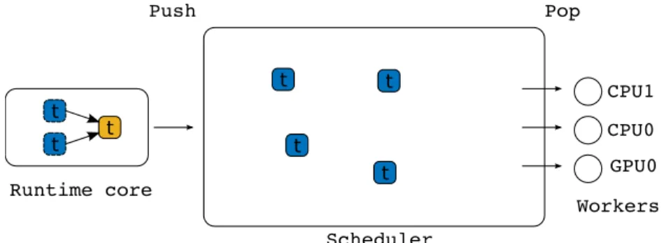
StarPU provides a framework for developing, tuning and experimenting various task scheduling policies in a portable way. Implementing a scheduler consists in creating a task container and defining the code that will be triggered each time a new task gets ready to be executed (push) or each time a processing unit has to select the next task to be executed (pop) as illustrated in Figure 2. The task container usually consists of a set of queues. The implementation of each queue may follow various strategies (e.g. FIFOs or LIFO) and sophisticated policies such as work-stealing may be implemented.

Figure 2: Designing a scheduling policy in StarPU.

Several built-in schedulers are available, ranging from greedy and work-stealing based policies to more elaborate schedulers implementing variants of the Heterogeneous Earliest Finish Time (HEFT) policy [25]. This latter family of schedulers usually relies on history-based performance models; the speed of data transfers is benchmarked right after installation of the runtime system whereas the performance of tasks is automatically collected by StarPU during the first executions of a given task. We show how we can benefit from this framework for designing a scheduling policy tailored for the multifrontal QR factorization in Section 4.

3

Frontal matrices partitioning strategies

One of the main challenges in implementing a multifrontal matrix factorization on GPU-accelerated multicore systems consists in finding front partitioning strategies allowing for the exploitation of both CPU and GPU resources. This issue results from the fact that GPUs are potentially able to deliver higher performance than CPUs by several orders of

magnitude but require coarse granularity operations to achieve it while a CPU reaches its peak with relatively small granularity tasks. Therefore we aim at designing a partitioning of frontal matrices that generates as much parallelism as possible in the DAG while delivering a sufficient amount of large granularity tasks in order to efficiently exploit GPUs.

In our study we consider the three front partitioning strategies illustrated in Figure 3: fine-grain, coarse-grain and hierarchical. The fine-grain partitioning (Figure 3(a)), which is the method of choice in work [18], consists in applying a regular 1D block partitioning on fronts and is therefore mainly suited for homogeneous architectures (e.g. multicore systems). The coarse grain partitioning (Figure 3(b)), where fine-grained panel tasks are executed on CPU and large-grain (as large as possible) update tasks are performed on GPU, corresponds to the algorithm developed in the MAGMA package [9] and aims at obtaining the best acceleration factor of computationally intensive tasks on GPU. In order to keep the GPU constantly busy, a static scheduling is used that allows for overlapping GPU and CPU computation thanks to a depth-1 lookahead technique; this is achieved by splitting the trailing submatrix update into two separate tasks of, respectively, fine and coarse granularity.

Figure 3: Front partitioning strategies. (a) Fine-grain. (b) Coarse-grain. (c) Hierarchical.

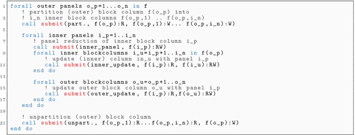
1 f o r a l l o u t e r p a n e l s o_p = 1 . . . o_n in f

! p a r t i t i o n ( o u t e r ) b l o c k c o l u m n f ( o_p ) i n t o

3 ! i_n i n n e r b l o c k c o l u m n s f ( o_p ,1) .. f ( o_p , i_n )

c a l l s u b m i t( p a r t . , f ( o_p ) : R , f ( o_p ,1) : W ... f ( o_p , i_n ) : W )

5

f o r a l l i n n e r p a n e l s i_p = 1 . . i_n

7 ! p a n e l r e d u c t i o n of i n n e r b l o c k c o l u m n i_p c a l l s u b m i t( i n n e r _ p a n e l , f ( i_p ) : RW )

9 f o r a l l i n n e r b l o c k c o l u m n s i_u = i_p + 1 . . i_n in f ( o_p )

! u p d a t e ( i n n e r ) c o l u m n i n _ u w i t h p a n e l i_p

11 c a l l s u b m i t( i n n e r _ u p d a t e , f ( i_p ) : R , f ( i_u ) : RW )

end do

13

f o r a l l o u t e r b l o c k c o l u m n s o_u = o_p + 1 . . o_n

15 ! u p d a t e o u t e r b l o c k c o l u m n o_u w i t h p a n e l i_p c a l l s u b m i t( o u t e r _ u p d a t e , f ( i_p ) : R , f ( o_u ) : RW ) 17 end do end do 19 ! u n p a r t i t i o n ( o u t e r ) b l o c k c o l u m n

21 c a l l s u b m i t( u n p a r t . , f ( o_p ,1) : R ... f ( o_p , i_n ) : R , f ( o_p ) : W )

end do

Although the fine-grain strategy generates enough parallelism in the DAG to reduce idle times, it results in a limited efficiency of GPU kernels as the tasks granularity is excessively small. On the the other end, the coarse-grain strategy allows for an optimal efficiency of kernels with respect to the problem size but reduces the parallelism and, combined with the static scheduling, increases the starvation of resources. The hierarchical partitioning of fronts (Figure 3(c)) is similar to the approach proposed in [26] and corresponds to a trade-off between parallelism and GPU kernel efficiency with task granularity suited for both types of resources. The front is first partitioned into coarse grain block-columns, referred to as outer block-columns, of width NBGPUsuitable for GPU computation (this happens at the moment

when the front is activated) and then each outer block-column is dynamically re-partitioned into inner block-columns of width NBCPU appropriate for the CPU only immediately before

being factorized. This is achieved through a dedicated partitioning task which is subject to dependencies with respect to the other, previously submitted, tasks that operate on the same data. When these dependencies are satisfied, StarPU ensures that the block being re-partitioned is in a consistent state, in case there are multiple copies of it. Furthermore, StarPU ensures that the partitioning is performed in a logical fashion: no actual copy is performed and there is no extra data allocated. The initial STF code corresponding to the QR factorization of a front (lines 14-21 in Figure 1(right)) is turned into the one proposed in Figure 4 for hierarchically partitioned fronts. We define inner and outer tasks depending on whether these tasks are executed on inner or outer block-columns. In order to ease the understanding we use different names for inner and outer updates although both types of tasks perform exactly the same operation and thus employ the same code.

Because the number of fronts in the elimination tree is commonly much larger than the number of working threads, the above-mentioned partitioning strategy is not applied to all of them. In our code we employ a technique similar to that proposed by Geist and Ng [27] that we describe in our previous work [23] under the name of logical tree pruning. Through this technique, we identify a layer in the elimination tree such that each subtree rooted at this layer is treated in a single task with a purely sequential code. This has a twofold advantage. First it reduces the number of generated tasks and, therefore, the runtime system overhead. Second, because we do not exploit node parallelism in these subtrees, we apply a coarse-grain partitioning of their fronts in order to maximize the granularity and subsequently the efficiency of GPU kernels. This could be achieved in a straightforward way by using the QR factorization routine of MAGMA for processing all the nodes in these subtrees; this, however, would result in a suboptimal choice because, as explained in Section 2.1 fronts have a staircase structure. Consequently we extended the MAGMA dgeqrf routine to take into account such a staircase structure. The assembly and panel operations within these sequential subtrees are executed on the CPU associated with the GPU worker thread (see Section 2.2) while update operations are handled by the GPU.

Concerning the memory consumption, the GPU can obviously be used only for those tasks whose footprint does not exceed the memory available on the device. For inner and outer updates the memory footprint is, respectively two inner panels and one inner plus one outer panel; the tasks that treat entire sequential subtrees, instead, are subject to the same memory constraint as the MAGMA kernels they rely on. This allows for using the GPU device on all the GPU-enabled tasks even for extremely large input problems (see Section 5.4).

4

Scheduling

Once the partitioning has been performed, one could statically assign the tasks of coarse granularity to GPUs and the ones of fine granularity to CPU cores. However, the variety of

front shapes and staircase structures combined with this hierarchical partitioning induces an important workload heterogeneity, making load balancing extremely hard to anticipate. For this reason, we chose to rely on a dynamic scheduling strategy. In the context of an heterogeneous architecture, the scheduler should be able to handle the workload hetero-geneity and distribute the tasks taking into account a number of factors including resource capabilities or memory transfers while ensuring a good load balance between the workers. Dynamic scheduling allows for dealing with the complexity of the workload and limit load imbalance between resources.

As discussed in Section 2.2, scheduling algorithms based on HEFT constitute a popular solution to schedule task graphs on heterogeneous systems. These methods consist in first ranking tasks (typically according to their position with respect to the critical path) and then assigning them to resources using a minimum completion time criterion. The main drawback of this strategy lies in the fact that the acceleration factor of tasks is ignored during the worker selection phase. In addition, the centralized decision during the worker selection potentially imposes a significant runtime overhead during the execution. A performance analysis conducted with the so-called dmdas StarPU built-in implementation of HEFT (and not reported here for a matter of conciseness) showed that these drawbacks are too severe for designing a high-performance multifrontal method.

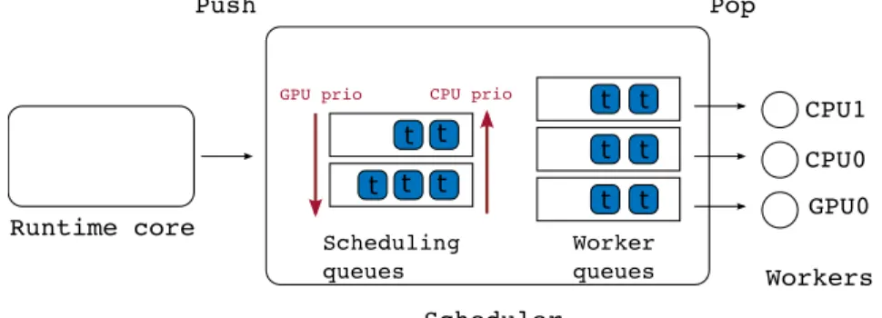
Instead, we implemented a scheduling technique known as HeteroPrio, first introduced in [28] in the context of Fast Multipole Methods (FMM). This technique is inspired by the observation that a DAG of tasks may be extremely irregular and alternate regions where concurrency is abundant with others where it is scarce. In the first case we can affect tasks to the units where they are executed the most effectively. In the second case, however, what counts most is to prioritize tasks which lie along the critical path because delaying their execution would result in penalizing stalls in the execution pipeline. As a result, in the HeteroPrio scheduler the execution is characterized by two states: a steady-state when the number of tasks is large compared to the number of resources and a critical-state in the opposite case.

Worker queues Scheduling

queues

Figure 5: HeteroPrio steady-state policy.

A complex, irregular workload, such as a sparse factorization, is typically a succession of steady and critical state phases. During a steady-state phase, tasks are pushed to dif-ferent scheduling queues depending on their expected acceleration factor (see Figure 5). In our current implementation, we have defined one scheduling queue per type of tasks (eight in total as listed in column 1 of Table 1). When they pop tasks, CPU and GPU work-ers poll the scheduling queues in different ordwork-ers. The GPU worker first polls scheduling queues corresponding to coarse-grain tasks such as outer updates (priority 0 on GPU in Table 1) because their acceleration factor is higher. On the contrary, CPU workers first poll scheduling queues of small granularity such as subtree factorizations or inner panels

(as well as tasks performing symbolic work such as activation that are critical to ensure progress). Consequently, during a steady-state, workers process tasks that are best suited for their capabilities. The detailed polling orders are provided in Table 1. Furthermore, to ensure fairness in the progress of the different paths of the elimination tree, tasks within each scheduling queue are sorted according to the distance (in terms of flop) between the corresponding front and root node of the elimination tree.

In the original HeteroPrio scheduler [28], the worker selection is performed right before popping the task in a scheduling queue following the previously presented rules. If data associated to the task are not present on the memory node corresponding to the selected worker then the task completion time is increased by the memory transfers. While the associated penalty is usually limited in the FMM case [28], preliminary experiments (not reported here for a matter of conciseness) showed that it may be a severe drawback for the multifrontal method. For the purpose of the present study, we have therefore extended the original scheduler by adding worker queues (one queue per worker) along with the scheduling queues as shown in Figure 5. When it becomes idle, a worker pops a task from its worker queue and then fills it up again by picking a new task from the scheduling queues through the polling procedure described above. The data associated with tasks in a worker queue can be automatically prefetched on the corresponding memory node while the corresponding worker is executing other tasks. If the size of the worker queues is too high, a task may be assigned to a worker much earlier than its actual execution, which may result in a sub-optimal choice. Therefore, because no additional benefit was observed beyond this value, we set this size to two in our experiments.

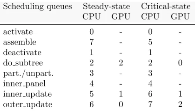
Scheduling queues Steady-state Critical-state CPU GPU CPU GPU

activate 0 - 0 -assemble 7 - 5 -deactivate 1 - 1 -do subtree 2 2 2 0 part./unpart. 3 - 3 -inner panel 4 - 4 -inner update 5 1 6 1 outer update 6 0 7 2

Table 1: Scheduling queues and polling orders in HeteroPrio.

When the number of tasks becomes low (with respect to a fixed threshold which is set depending on the amount of computational power of the platform), the scheduling algorithm switches to critical-state. CPU and GPU workers cooperate to process critical tasks as early as possible in order to produce new ready tasks quickly. For instance, because outer updates are less likely to be on the critical path, the GPU worker will select them last in spite of their high acceleration factor. The last two columns of Table 1 provide the corresponding polling order. Additionally, in this state, CPU workers are allowed to select a task only if its expected completion time does not exceed the total completion time of the tasks remaining in the GPU worker queue. This extra rule prevents CPU workers to select all the few available tasks at that moment and let the GPU idle whereas it could have finished to process them all earlier.

5

Experimental results

All the above discussed techniques have been implemented in the qr mumps solver on top of the StarPU runtime system and assessed on a set of eight matrices from the UF Sparse Matrix Collection1 _{plus one (matrix #1) from the HIRLAM}2 _{research program. These}

matrices are listed in Table 2 along with their size, number of nonzeroes and operation count obtained when applying a COLAMD fill-reducing column permutation.

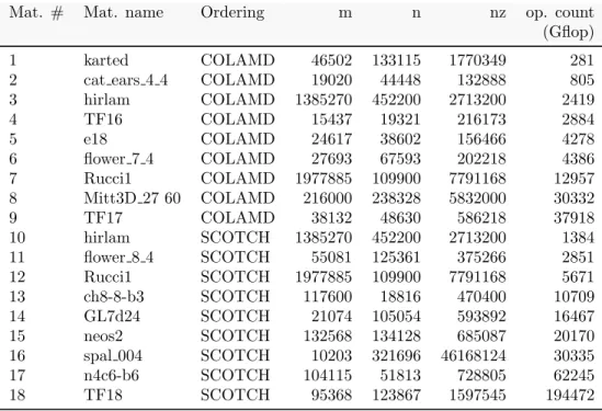
Mat. # Mat. name Ordering m n nz op. count (Gflop) 1 karted COLAMD 46502 133115 1770349 281 2 cat ears 4 4 COLAMD 19020 44448 132888 805 3 hirlam COLAMD 1385270 452200 2713200 2419 4 TF16 COLAMD 15437 19321 216173 2884 5 e18 COLAMD 24617 38602 156466 4278 6 flower 7 4 COLAMD 27693 67593 202218 4386 7 Rucci1 COLAMD 1977885 109900 7791168 12957 8 Mitt3D 27 60 COLAMD 216000 238328 5832000 30332 9 TF17 COLAMD 38132 48630 586218 37918 10 hirlam SCOTCH 1385270 452200 2713200 1384 11 flower 8 4 SCOTCH 55081 125361 375266 2851 12 Rucci1 SCOTCH 1977885 109900 7791168 5671 13 ch8-8-b3 SCOTCH 117600 18816 470400 10709 14 GL7d24 SCOTCH 21074 105054 593892 16467 15 neos2 SCOTCH 132568 134128 685087 20170 16 spal 004 SCOTCH 10203 321696 46168124 30335 17 n4c6-b6 SCOTCH 104115 51813 728805 62245 18 TF18 SCOTCH 95368 123867 1597545 194472

Table 2: The set of matrices used for the experiments.

The experiments were run on two platforms:

• Bunsen: includes one Intel Xeon E5-2650 processor (eight cores) accelerated with an Nvidia Kepler K40c GPU. In this case, the experiments were done with fixed values for the inner and outer block size of, respectively, 128 and 512; these values allow for a good average performance but may be rather far from the optimal.

• Sirocco: includes two Intel Xeon E5-2680 (twelve cores each) and one Nvidia Kepler

K40m GPU. On these platform all the block-size combinations in the set (nbgpu,nbcpu)={(256,128),

(256,256), (384,128), (384,384), (512,128), (512,256), (512,512) (768,128), (768,256), (768,384), (896,128), (1024,128), (1024,256), (1024,512) } were tested in order to evaluate the best achievable performance. For this platform, the results presented below are related to the best possible block-size combination.

5.1

Performance

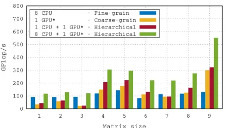
We compare the performance of the discussed front partitioning strategies for the multi-frontal factorization of our test set of sparse matrices. The results presented in Figure 6

1_{http://www.cise.ufl.edu/research/sparse/matrices/} 2_{http://hirlam.org}

show that the hierarchical partitioning offers the best performance and a speedup of up to 4.7 compared to the CPU only version on the Bunsen platform. When using one CPU along with the GPU, the performance becomes very low compared to the CPU only version for the smaller matrices as no tree parallelism is exploited during the factorization and also because the problem size leads to a limited acceleration of the factorization of fronts. A noticeable results in the factorization of matrix #9 is that the speed-up when using eight CPUs instead of one is greater than the peak performance offered by the additional CPUs. This is due to the fact that when multiple CPUs are available, the scheduling achieves a better matching between the characteristics of the tasks and the processing units whereas when only one CPU is available, the GPU is more likely to execute small granularity tasks.

0 100 200 300 400 500 600 700 800 1 2 3 4 5 6 7 8 9 GFlop/s Matrix size Performance -- Bunsen 8 CPU - Fine-grain 1 GPU* - Coarse-grain 1 CPU + 1 GPU* - Hierarchical 8 CPU + 1 GPU* - Hierarchical

Figure 6: Performance results on te Bunsen platform for qr mumps with three partitioning strategies: fine-grain, coarse-grain and hierarchical partitioning. GPU* indicates a GPU worker, i.e., with an associated CPU as explained in Section 2.2.

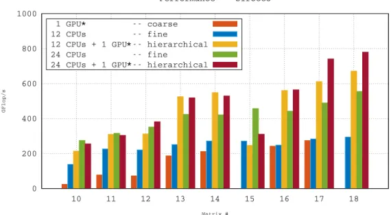
Figure 7 shows performance results on the Sirocco platform which confirm those obtained on the Bunsen one. Nonetheless it has to be noted that on Sirocco higher performance was achieved which proves that the code is well capable of exploiting heterogeneity as it took advantage of the extra performance provided by the CPUs.

5.2

Analysis

While the results presented above show the superiority of the hierarchical scheme with re-spect to the other proposed partitioning strategies, one may wonder how this scheme behaves in absolute. The most straightforward reference would be the cumulative peak performance over all computational units. This choice, however, does not take into account the fact that, due to their nature (be it their maximum granularity or the nature of operations they perform), tasks cannot be executed at the peak speed and may result in an excessively coarse bound on achievable performance. For this reason we decided to use a more accurate reference, the area bound tarea_{(p), which is obtained by solving a relaxed version of our}

scheduling problem built on the following assumptions: there are no dependencies between tasks; tasks are moldable (i.e. may be processed by multiple units); CPU-GPU memory transfers are instantaneous.

0 200 400 600 800 1000 10 11 12 13 14 15 16 17 18 GFlop/s Matrix # Performance -- Sirocco 1 GPU -- coarse 12 CPUs -- fine

12 CPUs + 1 GPU -- hierarchical 24 CPUs -- fine

24 CPUs + 1 GPU -- hierarchical

*

* *

Figure 7: Performance results on the Sirocco platform for qr mumps with three partitioning strategies: fine-grain, coarse-grain and hierarchical partitioning. GPU* indicates a GPU worker, i.e., with an associated CPU as explained in Section 2.2.

Figure 8 gives a pictorial example of how tarea(p) is defined on a simple execution with three resources (2 CPUs and 1 GPU).

Figure 8: Gantt chart. (a) Actual schedule. (b) Area schedule.

For a set of tasks Ω running on a set of P processors, we define αω

p as the share of work

in task ω processed by PU p and tω

p as the time spent by PU p processing its share of task ω.

Based on these definitions, tarea_{(p) can be computed as the solution of the following linear}

program

Linear Program 1 Minimize T such that, for all p ∈ P and for all ω ∈ Ω:

X ω∈Ω αω_ptω_p = tp≤ T P X p=1 αω_p = 1

For all tasks ω ∈ Ω and for all processes p ∈ P , tω

p is computed using performance

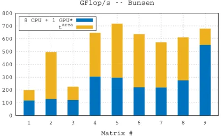
models automatically built by StarPU upon previous executions of the code The comparison between the performance obtained with the qr mumps execution time and tarea_{(p) is shown}

in Figure 9 for the test matrices; it must be noted that the reference performance is well below the architecture peak speed.

0 100 200 300 400 500 600 700 800 1 2 3 4 5 6 7 8 9 Matrix # GFlop/s -- Bunsen 8 CPU + 1 GPU* tarea

Figure 9: Performance results for qr mumps compared to theoretical performance bounds on the Bunsen platform.

A better understanding of the difference between the two performance measures in Fig-ure 9 can be achieved by decomposing t(p) into tt(p), tr(p) and ti(p), defined as, respectively,

the cumulative time spent in tasks, the cumulative time spent in the runtime and the cu-mulative idle time spent waiting for dependencies to be satisfied. Thanks to the prefetching feature implemented in our scheduler (see Section 4), most of the CPU-to-GPU (and vice-versa) memory transfers are hidden behind computation but, whenever this is not the case, the corresponding time is included in ti(p). This decomposition allows us to write the

parallel execution time as t(p) = (tt(p) + tr(p) + ti(p))/p and, consequently, the efficiency as

e(p) = eh tarea_{(p) × p} tt(p) · er tt(p) tt(p) + tr(p) · ep tt(p) + tr(p) tt(p) + tr(p) + ti(p) .

This expression allows us to decompose the efficiency as the product of three well defined effects. eh , which we call the “heterogeneity efficiency”, measures how well the assignment

of tasks to processing units matches the one computed by the linear program above and, therefore, how well the capabilities of each unit have been exploited. ep, which we call the

“pipeline efficiency” measures how much concurrency is available (depending on the size and structure of the input matrix and on the chosen block sizes) and how well it is exploited to feed the processing units. Note that eh can be greater than 1 which happens when the

GPU is overloaded; this inevitably results in CPUs starvation and, thus, a poorer pipeline efficiency. In essence, the product of ehand epcan be seen as a measure of the quality of the

scheduling and is always lower than or equal to 1. Finally, er , which we call the “runtime

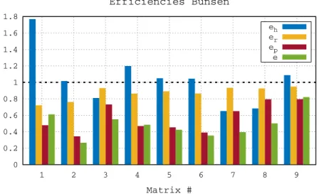
efficiency”, measures how the overhead of the runtime system reduces the global efficiency. Figure 10 shows the efficiency analysis for our code on the test matrices. The run-time overhead becomes relatively smaller and smaller as the size of the problems increases: whereas this overhead is penalizing on smaller size matrices, it becomes almost negligible on the largest ones. These results also show that our scheduling policy makes a relatively

0 0.2 0.4 0.6 0.8 1 1.2 1.4 1.6 1.8 1 2 3 4 5 6 7 8 9 Matrix # Efficiencies Bunsen e_h e_r e_p e

Figure 10: Efficiency of qr mumps on the matrix test set on the Bunsen platform.

good job in assigning tasks to the units where they can be executed more efficiently, apart for the case of matrix #1. In most cases, the most penalizing effect on the global efficiency is the pipeline efficiency ep. This is mainly due to a lack of concurrency resulting from

the choice of partitioning. This choice aims at achieving the best compromise between the efficiency of kernels and the amount of concurrency; it must be noted that epcould certainly

be improved by using a finer grain partitioning but this would imply a worse efficiency of the tasks and thus, as a consequence, higher values for both tt(p) and tarea(p). We are working

at extending our efficiency analysis in a way to show the loss of tasks efficiency due to the applied partitioning. It must also be noted that fixed inner and outer block sizes have been chosen for all our experiments; although we have used values that deliver a good average performance, custom values for each problem could yield considerable improvements.

5.3

Multi-streaming

Choosing the good size for inner and outer operations is a delicate act of balance between concurrency and efficiency of operations; this task is difficult mostly because of the very high granularity of operations required by GPUs. The use of multiple streams – a feature available on relatively recent GPUs – allows for achieving a better occupancy of the device even for smaller grained tasks thanks to the concurrent execution of GPU tasks; this leads to a better compromise between efficiency of tasks and concurrency and, as a consequence, to higher performance. In addition, multiple streams allow for a better exploitation of tree and node parallelism by enabling the concurrent processing tasks, possibly from different fronts of the elimination tree, on the same GPU. We report in Table 3, preliminary results when exploiting the multistream feature of the GPU (we only use two streams). The impact of the multistream feature on small matrices is marginal while the performance gap between the mono and multi stream version tend to increase with the problem size.

5.4

Comparison with a state-of-the-art GPU solver

In this section we provide a comparison of our solver with the GPU-enabled version of the spqr solver [1]. This solver is specifically designed for a GPU-only execution where all

Factorize time (s)

Bunsen Sirocco

Mat. # 1 stream 2 streams Mat. # 1 stream 2 streams 1 2.401E+00 2.425e+00 10 1.237E+01 1.238E+01 2 6.242E+00 6.678e+00 11 1.034E+01 9.044E+00 3 1.989E+01 1.938E+01 12 2.151E+01 2.489E+01 4 9.471E+00 1.078E+01 13 2.125E+01 1.904E+01 5 1.445E+01 1.492E+01 14 2.915E+01 2.658E+01 6 1.984E+01 2.069E+01 15 1.353E+02 1.514E+02 7 5.897E+01 4.923E+01 16 4.962E+01 4.395E+01 8 1.101E+02 8.357E+01 17 1.114E+02 1.010E+02 9 6.870E+01 6.104E+01 18 3.312E+02 3.022E+02

Table 3: Factorization time for the test matrices with qr mumps using 1 and 2 streams. On the last column, the factorization times for the spqr solver on the Bunsen and Sirocco platforms.

the operations (linear algebra kernels as well as assemblies) are executed on the GPU; one core is used to drive the activity of the GPU through a technique referred to as bucket scheduling. Essentially, the factorization proceeds in sequential steps where, at each step, the bucket scheduler builds a list of independent and heterogeneous tasks and transmits it to the GPU; on the GPU side, a single kernel is launched which is capable of executing all the different types of tasks in the list provided by the bucket scheduler. In spqr fronts are allocated and assembled directly on the GPU; this strategy has the great benefit of improving performance by relieving the code from the burden of moving data back and forth from the host to the device memory. Nonetheless, this requires a careful handling of the data because of the limited size of the GPU memory. For this reason, in spqr the elimination tree is statically (at the analysis time) split into stages such that each piece fits in the GPU memory; these pieces are sequentially processed in successive steps. It must be noted that the smallest possible stage is formed by a family, i.e., a front plus its children which are needed to assemble the front itself. Therefore, spqr will not be able to factorize a matrix whose elimination tree includes a family that does not fit in the GPU memory.

A comparison of the execution time of qr mumps and spqr is shown in Table 4. In both cases COLAMD ordering is applied resulting in the same amount of flop during factorization. The performance results show that, despite the additional logic needed to exploit both the GPU and the CPUs and to processes problems that require higher memory than what is available on the GPU, our solver achieves a better performance than spqr on the largest size problems. It must be noted that spqr could not factorize matrices #8 and #9 because of memory consumption issues. Our solver, instead, always runs to completion as long as enough memory is available on the host and will be capable of using the GPU for all tasks whose memory footprint does not exceed the GPU memory size, as explained in Section 3. In two cases (matrices #3 and #7) the spqr solver returned an erroneous solution.

6

Conclusion and future work

We have presented a multifrontal QR factorization technique for single-node architectures equipped with multicore processors and GPUs. Our approach relies on the simplicity and expressiveness of the STF paradigm and on the robustness and performance of modern runtime systems that implement this parallel programming model. Using the features of

# Mat. name Factorize time (s) best(1,2) streams spqr 1 karted 2.401 2.721 2 cat ears 4 4 6.242 5.281 3 hirlam 19.384 ∗ 4 TF16 9.471 14.373 5 e18 14.451 18.263 6 flower 7 4 19.841 22.004 7 Rucci1 49.237 ∗ 9 TF17 61.040 ∗∗

Table 4: Factorization time on the Bunsen platform for the test matrices with qr mumps using either 1 or 2 streams and with spqr. ∗ means that the solver returned an erroneous solution and ∗∗ means that the memory requirement for these matrices exceeded the GPU memory size.

these efficient tools, we defined a dynamic, hybrid partitioning of the data that produces a good mixture of fine and large granularity tasks that aims at maximizing the efficiency of operations on both the CPUs and the GPU while still achieving a sufficient amount of concurrency. In order to cope with the heterogeneity of the workload and of the underlying architecture, we have implemented a scheduling policy capable of deploying tasks on the units where they can be executed the most efficiently when concurrency is abundant while resorting to a more conservative approach where critical tasks are prioritized in the case where parallelism is scarce. We have presented experimental results assessing the effective-ness of the proposed techniques and provided a fine and detailed analysis of the behavior of our solver.

Our work shows that the STF programming model is suitable for handling extremely heterogeneous workloads that feature tasks of very different nature and granularity, and to deploy it on a heterogeneous architecture that includes units with different processing capabilities while relieving the programmer from the burden of manually handling the mem-ory transfers and of ensuring the consistency of multiple data copies. This programming model as well as the rich set of features of modern runtime systems, ease the development of complex techniques for dealing with the irregularity of the workload and the heterogeneity of the architecture.

This work opens up a large number of perspectives and allows for further research and developments. First, and most naturally, the case of a single node equipped with multiple GPUs should be addressed. It must be noted that our solver can be executed on such an architecture right away: the runtime system will take care of dispatching tasks to the multiple GPUs as well as to the CPUs. However, most likely this will not lead to an acceptable performance because the scheduling as well as the partitioning techniques must be adapted to this case.

A block-column partitioning is not well suited for the cases where frontal matrices are extremely over-determined (which is often the case for the multifrontal QR method); in such cases a 2D blocking of frontal matrices can be applied and Communication-Avoiding factorization algorithms can be used to improve the amount of concurrency. This technique has the major drawback of considerably reducing the granularity of operations and therefore much better care must be taken when partitioning the data and scheduling the resulting tasks. This is a natural extension of our previous work on multicore architectures [17]; the memory-aware task scheduling discussed therein can also be adapted to the case of GPU-accelerated architectures.

Another possible evolution of our solver is towards distributed memory, parallel systems: modern runtime systems, such as StarPU, are capable of handling this type of architectures by transparently managing the transfer of data between nodes through the network. A solver that implements all the above-mentioned features is our ultimate objective.

7

Acknowledgments

This work is supported by the Agence Nationale de la Recherche, under grant ANR-13-MONU-0007.

References

[1] S. N. Yeralan, T. A. Davis, and S. Ranka, “Sparse QR factorization on the GPU,” University of Florida, Tech. Rep., 2015, technical report.

[2] C. D. Yu, W. Wang, and D. Pierce, “A CPU-GPU hybrid approach for the unsymmetric multifrontal method,” Parallel Comput., vol. 37, pp. 759–770, Dec. 2011.

[3] K. Kim and V. Eijkhout, “Scheduling a parallel sparse direct solver to multiple GPUs,” in Parallel and Distributed Processing Symposium Workshops PhD Forum (IPDPSW), 2013 IEEE 27th International, May 2013, pp. 1401–1408.

[4] J. Hogg, E. Ovtchinnikov, and J. Scott, “A sparse symmetric indefinite direct solver for GPU architectures,” STFC Rutherford Appleton Lab., Tech. Rep. RAL-P-2014-006, 2014.

[5] X. Chen, L. Ren, Y. Wang, and H. Yang, “GPU-accelerated sparse LU factorization for circuit simulation with performance modeling,” Parallel and Distributed Systems, IEEE Transactions on, vol. 26, no. 3, pp. 786–795, March 2015.

[6] P. Sao, R. W. Vuduc, and X. S. Li, “A distributed CPU-GPU sparse direct solver,” in Euro-Par 2014 Parallel Processing, 2014, pp. 487–498.

[7] A. Buttari, J. Langou, J. Kurzak, and J. Dongarra, “A class of parallel tiled linear algebra algorithms for multicore architectures,” Parallel Comput., vol. 35, pp. 38–53, January 2009.

[8] G. Quintana-Ort´ı, E. S. Quintana-Ort´ı, R. A. V. D. Geijn, F. G. V. Zee, and E. Chan, “Programming matrix algorithms-by-blocks for thread-level parallelism,” ACM Trans. Math. Softw., vol. 36, no. 3, 2009.

[9] E. Agullo, J. Demmel, J. Dongarra, B. Hadri, J. Kurzak, J. Langou, H. Ltaief, P. Luszczek, and S. Tomov, “Numerical linear algebra on emerging architectures: The PLASMA and MAGMA projects,” Journal of Physics: Conference Series, vol. 180, no. 1, p. 012037, 2009.

[10] G. Bosilca, A. Bouteiller, A. Danalis, T. Herault, P. Luszczek, and J. Dongarra, “Dense linear algebra on distributed heterogeneous hardware with a symbolic dag approach,” Scalable Computing and Communications: Theory and Practice, 2013.

[11] C. Augonnet, S. Thibault, R. Namyst, and P.-A. Wacrenier, “StarPU: A Unified Platform for Task Scheduling on Heterogeneous Multicore Architectures,” Concurrency and Computation: Practice and Experience, Special Issue: Euro-Par 2009, vol. 23, pp. 187–198, Feb. 2011.

[12] G. Bosilca, A. Bouteiller, A. Danalis, T. H´erault, P. Lemarinier, and J. Dongarra, “DAGuE: A generic distributed DAG engine for high performance computing,” Parallel Computing, vol. 38, no. 1-2, pp. 37–51, 2012.

[13] R. M. Badia, J. R. Herrero, J. Labarta, J. M. P´erez, E. S. Quintana-Ort´ı, and G. Quintana-Ort´ı, “Parallelizing dense and banded linear algebra libraries using SMPSs,” Concurrency and Computation: Practice and Experience, vol. 21, no. 18, pp. 2438–2456, 2009.

[14] E. Hermann, B. Raffin, F. Faure, T. Gautier, and J. Allard, “Multi-GPU and multi-CPU parallelization for interactive physics simulations,” in Euro-Par (2), 2010, pp. 235–246.

[15] X. Lacoste, M. Faverge, P. Ramet, S. Thibault, and G. Bosilca, “Taking advantage of hybrid systems for sparse direct solvers via task-based runtimes,” IEEE, Phoenix, AZ, 05/2014 2014.

[16] K. Kim and V. Eijkhout, “A parallel sparse direct solver via hierarchical DAG schedul-ing,” ACM Trans. Math. Softw., vol. 41, no. 1, pp. 3:1–3:27, Oct. 2014.

[17] E. Agullo, A. Buttari, A. Guermouche, and F. Lopez, “Implementing multifrontal sparse solvers for multicore architectures with Sequential Task Flow runtime systems,” IRIT, Universit´e Paul Sabatier, Toulouse, Rapport de recherche IRI/RT–2014-03–FR, novembre 2014, submitted to ACM Transactions On Mathematical Software.

[18] ——, “Multifrontal QR factorization for multicore architectures over runtime systems,” in Euro-Par 2013 Parallel Processing. Springer Berlin Heidelberg, 2013, pp. 521–532.

[19] T. A. Davis, “Algorithm 915, SuiteSparseQR: Multifrontal multithreaded rank-revealing sparse QR factorization,” ACM Trans. Math. Softw., vol. 38, no. 1, pp. 8:1–8:22, Dec. 2011.

[20] I. S. Duff and J. K. Reid, “The multifrontal solution of indefinite sparse symmetric linear systems,” ACM Transactions On Mathematical Software, vol. 9, pp. 302–325, 1983.

[21] R. Schreiber, “A new implementation of sparse Gaussian elimination,” ACM Transac-tions On Mathematical Software, vol. 8, pp. 256–276, 1982.

[22] P. R. Amestoy, I. S. Duff, and C. Puglisi, “Multifrontal QR factorization in a mul-tiprocessor environment,” Int. Journal of Num. Linear Alg. and Appl., vol. 3(4), pp. 275–300, 1996.

[23] A. Buttari, “Fine-grained multithreading for the multifrontal QR factorization of sparse matrices,” SIAM Journal on Scientific Computing, vol. 35, no. 4, pp. C323–C345, 2013.

[24] J. Kurzak and J. Dongarra, “Fully dynamic scheduler for numerical computing on multicore processors,” LAPACK working note, vol. lawn220, 2009.

[25] H. Topcuouglu, S. Hariri, and M.-y. Wu, “Performance-effective and low-complexity task scheduling for heterogeneous computing,” IEEE Transactions on Parallel and Dis-tributed Systems, vol. 13, no. 3, pp. 260–274, Mar 2002.

[26] W. Wu, A. Bouteiller, G. Bosilca, M. Faverge, and J. Dongarra, “Hierarchical dag scheduling for hybrid distributed systems,” in 29th IEEE International Parallel & Dis-tributed Processing Symposium (IPDPS), Hyderabad, India, May 2015.

[27] A. Geist and E. G. Ng, “Task scheduling for parallel sparse Cholesky factorization,” Int J. Parallel Programming, vol. 18, pp. 291–314, 1989.

[28] E. Agullo, B. Bramas, O. Coulaud, E. Darve, M. Messner, and T. Takahashi, “Task-based FMM for heterogeneous architectures,” Inria, Research Report RR-8513, Apr. 2014.