A successive constraint method with minimal offline constraints for lower bounds of parametric coercivity constant

(1)

HAL Id: hal-00609212

https://hal.archives-ouvertes.fr/hal-00609212

Preprint submitted on 18 Jul 2011

HAL is a multi-disciplinary open access

archive for the deposit and dissemination of

sci-entific research documents, whether they are

pub-lished or not. The documents may come from

teaching and research institutions in France or

abroad, or from public or private research centers.

L’archive ouverte pluridisciplinaire HAL, est

destinée au dépôt et à la diffusion de documents

scientifiques de niveau recherche, publiés ou non,

émanant des établissements d’enseignement et de

recherche français ou étrangers, des laboratoires

publics ou privés.

constraints for lower bounds of parametric coercivity

constant

Sylvain Vallaghé, Michel Fouquembergh, Annabelle Le Hyaric, Christophe

Prud’Homme

To cite this version:

Sylvain Vallaghé, Michel Fouquembergh, Annabelle Le Hyaric, Christophe Prud’Homme. A successive

constraint method with minimal offline constraints for lower bounds of parametric coercivity constant.

2011. �hal-00609212�

(2)

/

A successive constraint method with minimal offline constraints for lower

bounds of parametric coercivity constant. Une m´ethode par contraintes

successives avec un minimum de contraintes hors ligne pour les bornes

inférieures des constantes de coercivité à dépendance paramétrique.

Sylvain Vallagh´ea_{, Michel Fouquembergh}b_{, Anabelle Le Hyaric}b_{, Christophe Prud’homme}a

a_{Laboratoire Jean Kuntzmann, Universit´e Joseph Fourier Grenoble 1, BP 53 38041 Grenoble Cedex 9, France} b_{EADS France Innovation Works, 12 rue Pasteur BP 76 92152 Suresnes Cedex, France}

Abstract

A posteriori error estimates are a key ingredient for the certified reduced basis method. Sharp error bounds rely on the construction of lower bounds for the coercivity or inf-sup stability constant. The Successive Constraint Method (SCM) has been previously proposed to compute such lower bounds, using an effi-cient Offline-Online strategy. We present in this article some modifications to the SCM to get rid of user-dependent parameters, which also improve convergence and reduce the computational cost of the method.

Les estimateurs d’erreur a posteriori sont un élément clé de la méthode des bases réduites certifiées. L’ob-tention d’estimateurs précis repose sur la construction de bornes inférieures pour la constante de coercivité ou de stabilité inf-sup. La Méthode par Contraintes Successives (SCM) a été proposée afin de calculer de telles bornes inférieures, en utilisant une stratégie efficace hors ligne-en ligne. Dans cet article, nous présentons certaines modifications à la SCM afin de se passer de paramètres dépendant de l’utilisateur. Ces modifications permettent également d’avoir une convergence plus rapide de la méthode, ainsi qu’un gain computationel significatif.

Keywords: Reduced basis method, Successive constraint method, Méthode bases réduites, Méthode par contraintes successives

1. Successive constraint method

This section describes the Successive Constraint Method (SCM) as first introduced in [1] and then im-proved in [2].

Starting from an affine bilinear form

a(w, v; µ) = Q X

q=1

(3)

over which (1) is feasible. First we set the design space for the minimisation problem (1). We introduce B =QQ q=1 h infw∈XN aq(w,w) kwk2 X ; supw∈XN aq(w,w) kwk2 X i Ξ =nµi∈ D; i = 1, ..., J o and CK = n µi∈ Ξ; i = 1, ..., K o ⊂ Ξ

Ξis a fine sampling of D. CK will be constructed using a greedy algorithm. Finally we denote PM(ν; E) the set of M points closest to ν in the set E.

1.1. Lower bounds

Given Mα,M+∈ N we are now ready to define YLBand αLB

YLB(ν; CK) = n y ∈ B|PQ q=1θq(ν′)yq≥ αN(ν′), ∀ν′∈ PMα(ν; CK) PQ q=1θq(ν ′ )yq≥ αLB(ν′; CK−1), ∀ν′∈ PM+(ν; Ξ\CK) o (2)

αLB(ν; CK) = infy∈Y_{LB(ν;CK )}Jobj(ν; y) (3) (3) is in fact a linear program with Q design variables, yq, and 2Q + Mα+ M+constraints online. It requires

the construction of CKoffline.

1.2. Upper bounds

YUB(CK) = n

y∗(µk), 1 ≤ k ≤ K o

with y∗(ν) = argminy∈YJobj(ν; y) αUB(ν; CK) = infy∈YUB(CK)J

obj

(ν; y) (4)

YUBrequires K eigensolves to compute the eigenmode ηkassociated with wk,k =1, ..., K and KQN inner products to compute the y∗q(wk) =

aq(ηk,ηk) kηkk2

XN

,k =1, ..., K offline . Then (4) is a simple enumeration online.

1.3. Construction of CK Given Ξ and ǫ ∈ [0; 1] While maxν∈Ξ αUB(ν;C_αK)−αLB(ν;CK) UB(ν;CK) > ǫ • µK+1=argmaxν∈Ξ αUB (ν;CK)−αLB(ν;CK) αUB(ν;CK) • CK+1= CK∪ {µK+1}, K ← K + 1 2. Discarding Mαand M+

For the computation of the lower bound, the two parameters Mαand M+must be set by the user, who is

supposed to have at least a basic knowledge of the SCM and what these parameters are meant to be. This is quite disappointing as the SCM is part of a framework for reduced basis a posteriori error computation, which should be usable like a black box. Moreover, even for someone familiar with the SCM, it is not straightforward to tune these parameters. Thus we propose a modification of the SCM which does not need the parameters Mαand M+, and gives a faster convergence.

(4)

2.1. Offline construction of CK

The constraints of the LP (2) for a given ν are basically corresponding to the definition of the coercivity constant taken at neighboring points ν′ of ν. For some of the first kind, the actual coercivity constant has been computed, (ν′ ∈ PMα(ν; CK)), for others of the second kind, only a lower bound is available

(ν′ ∈ PM+(ν; Ξ\CK)). Actually, when building the CK spaces, the lower bound estimates are rather poor,

at least for the first iterations. So the constraints of the second kind are not as good as the constraints of the first kind. Therefore, the first idea is to completely drop M+ and to keep only the constraint of the

second kind for ν′= ν, which enforces the monotonic decreasing of the stopping criterion. The next idea to get rid of Mα is to keep in mind that in a LP with Q variables, there are at most Q active constraints

when the minimum is reached. It is also straigthforward to see that among all constraints of the first kind, if a constraint is not active at rank K, it will not be active for all ranks J ≥ K. So while building the

CK spaces, we can keep track of these active constraints (of the first kind), which is easy because there is only to look if the new constraint given by µK is active. So we never get more than Q constraints of the first kind, therefore Mαis not needed anymore. One can note that there is no guarantee that the active

constraints correspond to the neighboring points ν′ _{∈ P}

Mα(ν; CK). As a consequence, taking the active

constraints instead of the neighboring constraints will give at least the same results, but more likely better results. Moreover, computing neighbors can be expensive if the trial sampling is big, this problem vanishes when considering the active constraints. To make things clear, with these modifications the space YLB at

iteration K now reads :

YLB(ν; CK) = n y ∈ B| PQ q=1θq(ν ′ )yq≥ αN(ν′), ∀ν′∈ A(ν; CK−1) PQ q=1θq(µK)yq≥ α N (µK) o

where A(ν; CK−1) denotes the set of active constraints at minimum for the computation of αLB(ν; CK−1).

After αLB(ν; CK) is computed, we check which constraints are active among A(ν; CK−1) ∪ µKand store the active ones in A(ν; CK).

2.2. Online computation of αLB

For the online computation of αLB(ν), we start from the same idea : the best constraints are from the

first kind, and only a few are active. But in this case, we have to deal with ν < Ξ, so the active set of constraints has not been built during the construction of CK. So to be sure to have the best constraints, one can use all the µk∈ CK. This is a rather brute force approach, but the computation is not so expensive as it corresponds to a linear program with few variables and many constraints, so it can be solved very rapidly by considering the dual problem.

3. A short example

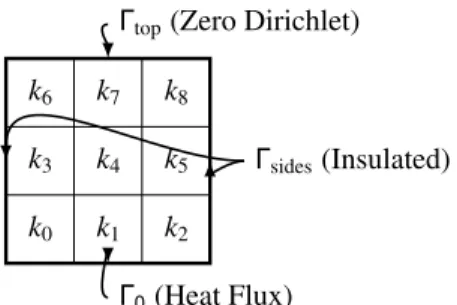
We illustrate our modifications on a simple 2D steady-state diffusion equation ∇ · (k∇u) = 0, in a square domain where k is piecewise constant as described in figure 1 (the thermal block problem [3]). The

ki,i =1..9 are the parameters of the PDE. One shall note that the problem is parametrically coercive, which means that in the affine decomposition

∀µ ∈ D, θq(µ) > 0 and ∀w ∈ XN,aq(w, w) ≥ 0 1 ≤ q ≤ Q.

So in this case, a lower bound for the coercivity constant can easily be computed without the need of the SCM [3]. We still consider the thermal block as a toy example to show the advantage of our proposed

(5)

avoided with the proposed SCM.

As described above, our modifications could be a drawback for online computation, because in this case taking the best constraints means taking all the constraints from CK, i.e. K constraints. On this example, for K = 1500, it took 1mn to compute online 105_{different lower bounds, so it does not appear to be much}

of a problem.

Γ0(Heat Flux)

Γtop(Zero Dirichlet)

Γsides(Insulated)

k0 k1 k2

k3 k4 k5

k6 k7 k8

Figure 1: Domain geometry. G´eom´etrie du domaine.

0.01 0.1 1 0 200 400 600 800 1000 1200 1400 1600 SCM with neighbors proposed SCM

Figure 2: Value of the stopping criterion with respect to K. Valeur du crit`ere d’arrˆet en fonction de K.

Acknowledgements

The authors thank the ANR and the OPUS project for the funding of this work. References

[1] D. Huynh, G. Rozza, S. Sen, A. Patera, A successive constraint linear optimization method for lower bounds of parametric coercivity and inf-sup stability constants, CR Acad Sci Paris (345) (2007) 473–478.

[2] Y. Chen, J. S. Hesthaven, Y. Maday, J. Rodr´ıguez, Improved successive constraint method based a posteriori error estimate for reduced basis approximation of 2d maxwell’s problem, Elsevier ScienceSubmitted.

[3] S. Sen, Reduced-basis approximation and a posteriori error estimation for many-parameter heat conduction problems, Numerical Heat Transfer, Part B: Fundamentals 54 (5) (2008) 369–389.