Alternative Activity Pattern Generation
for Stated Preference Surveys
The MIT Faculty has made this article openly available. Please share how this access benefits you. Your story matters.
Citation He, He et al. “Alternative Activity Pattern Generation for Stated Preference Surveys” Transportation Research Record, vol. 2672, no. 47, 2018, pp. 135-145 © 2018 The Author(s)
As Published https://dx.doi.org/10.1177/0361198118782760 Publisher SAGE Publications
Version Author's final manuscript
Citable link https://hdl.handle.net/1721.1/125659
Terms of Use Creative Commons Attribution-Noncommercial-Share Alike Detailed Terms http://creativecommons.org/licenses/by-nc-sa/4.0/
ALTERNATIVE ACTIVITY PATTERN GENERATION FOR STATED PREFERENCE 1 SURVEYS 2 3 4 5 He He 6
Massachusetts Institute of Technology 7
77 Massachusetts Avenue, Room 9-549, Cambridge, MA 02139 8
Tel: 617-955-3922; Email: [email protected] 9
10 11
Bilge Atasoy 12
Massachusetts Institute of Technology 13
77 Massachusetts Avenue, Room 1-180, Cambridge, MA 02139 14
Tel: 617-324-7197; Email: [email protected] 15
16 17
J. Cressica Brazier 18
Massachusetts Institute of Technology 19
77 Massachusetts Avenue, Room 9-549, Cambridge, MA 02139 20
Tel: 510-502-8032; Email: [email protected] 21
22 23
P. Christopher Zegras 24
Massachusetts Institute of Technology 25
77 Massachusetts Avenue, Room 10-403, Cambridge, MA 02139 26
Tel: 617-452-2433; Email: [email protected] 27
28 29
Moshe Ben-Akiva 30
Massachusetts Institute of Technology 31
77 Massachusetts Avenue, Room 1-181, Cambridge, MA 02139 32
Tel: 617-253-5324; Email: [email protected] 33
34 35 36
Word count: 6250 words text + 5 tables/figures x 250 words (each) = 7500 words 37
38 39
Submission Date: November 15, 2017. 40
ABSTRACT 1
We present a systematic method for generating activity-driven, multi-day alternative activity 2
patterns that form choice sets for stated preference surveys. An activity pattern consists of 3
information about an individual’s activity agenda, travel modes between activity episodes, and 4
the location and duration of each episode. The proposed method adjusts an individual’s observed 5
activity pattern using a hill-climbing algorithm, an iterative algorithm that finds local optima, to 6
search for the best response to hypothetical system changes. The multi-day approach allows for 7
flexibility to reschedule activities on different days and thus presents a more complete view of 8
demand for activity participation, as these demands are rarely confined to a single day in reality. 9
As a proof-of-concept, we apply the method to a multi-day activity-travel survey in Singapore 10
and consider the hypothetical implementation of an on-demand AV service. The demonstration 11
shows promising results with the algorithm exhibiting overall desirable behavior with reasonable 12
responses. In addition to representing the individual’s direct response, the use of observed 13
patterns also reveals the propagation of impacts, i.e. indirect effects, across the multi-day activity 14
pattern. 15
16
Keywords: Activity Patterns, Activity Rescheduling, Stated Preference Survey, Choice Set
17
Generation.
18 19
INTRODUCTION 1
Individuals generally do not make decisions to travel in isolation. Rather, they make these 2
choices simultaneously with, or as a result of, decisions to participate in activities. Accounting 3
for the motivations underlying individuals’ activity-travel behavior has become increasingly 4
recognized as essential to understanding today’s dynamic urban systems. This activity-based lens 5
is particularly useful for examining complex behavior, such as trip chaining, discretionary travel, 6
as well as the impacts of the range of “soft” measures associated with mobility management. 7
Considering the growing popularity of flexible work hours and shared on-demand modes, and 8
the potentially disruptive changes associated with autonomous vehicles (AVs) and mobility as a 9
service, we need better ways to understand how such innovations will influence individuals’ 10
demand for activities and, ultimately, the performance of the mobility and broader urban system. 11
To understand the possible implications of new products and services “unfamiliar” to a 12
consumer, researchers have long used the stated preference (SP) survey. Travel behavior analysis 13
often uses SP surveys to, say, understand how users might respond to a new mode, such as high 14
speed rail, or infrastructures, such as bike lanes. Such analyses, however, tend to be trip-focused 15
– conditional on a trip being made. New mobility innovations might, however, impact 16
individuals’ activity implementation plans or schedules by, for example, allowing more time to 17
partake in discretionary activities in a new location. Thus, understanding the process by which 18
individuals and households schedule their activities remains a core challenge in inferring 19
responses to new mobility or activity options. Even though activity scheduling is something that 20
nearly everyone actually does, to some degree, on a daily basis, formalizing and generalizing it 21
analytically is difficult. Activity scheduling is a multidimensional task that requires the decision 22
maker to choose a number of activities to complete, the sequence of these activities, the time, 23
duration, and location of each activity, and, when relevant, the mode of travel and route between 24
activity locations. Even assuming a reasonable discretization of time and space, the resulting 25
number of possible combinations is both computationally demanding and too large for any 26
person to feasibly consider, cognitively. Generating alternative activity patterns, thus, must aim 27
to be computationally efficient, while mimicking people’s actual decision-making processes. 28
In this paper, we propose a systematic method for generating alternative activity patterns 29
that will form choice sets for stated preference surveys within an activity-based modeling 30
framework. The method takes advantage of detailed multi-day activity diaries collected using 31
Future Mobility Sensing (FMS), a smartphone-based activity-travel survey platform (1). We start 32
with individuals’ revealed activity-travel patterns as the base for the new activity patterns. Then, 33
using the proposed method, we adjust the patterns in response to hypothetical scenarios. In 34
addition to representing the individual’s direct response, the use of observed patterns also reveals 35
the propagation of impacts across a multi-day activity pattern. Here, we review existing work 36
addressing the challenges of generating alternative activity patterns. We then present the new 37
method and the issues we considered in its development, and finally we show the results of a 38
proof-of-concept application of the proposed method using an activity-travel survey conducted in 39 Singapore. 40 41 BACKGROUND 42
Since the inception of the activity-based approach to travel demand modeling, researchers have 43
proposed and operationalized numerous activity-based frameworks. Each has taken on the 44
challenge of activity scheduling. Early work established that proposed activity-based models 45
must recognize and take into account the decision-making behavior of individuals and 46
households (2,3). Furthermore, they must be complete in scope, i.e. have sufficiently high 47
resolution and flexibility to capture the behavioral changes of interest. Lastly, they must be 1
feasible and practical to operationalize. Early frameworks applied mathematical programming 2
and neural networks in attempts to manage the complexity of the problem (4,5). However, these 3
methods did not simulate how people actually plan their schedules. More recent modelling 4
frameworks have used more sophisticated ways of representing planning and decision-making 5
processes. These approaches have generally fallen on a spectrum between entirely econometrics-6
based methods, building on discrete choice theory, e.g. SimMobility (6), to largely rule-based 7
methods that build on decision heuristics, e.g. TASHA (7,8) and ALBATROSS (9). Most 8
modelling frameworks can be considered hybrids, applying a combination of heuristics and 9
econometrics or at least using the concept of utility-maximization to simulate rationality. Pinjari 10
and Bhat provide a comprehensive overview of activity-based modelling frameworks (10). 11
A major challenge to operationalizing activity-based models has to do with realistically 12
representing how individuals schedule activities and, thus, what alternative activity patterns 13
might exist for a given individual. For the purposes of an activity-based SP survey, aimed at 14
understanding how an individual’s mode and activity preferences might change in the face of 15
new alternatives, realism would be gained by presenting activity pattern alternatives based on 16
respondents’ observed activity patterns. This requires methods that can capitalize on the 17
availability of existing patterns and estimate the utility of activities for a given individual. The 18
AMOS model, a micro-simulator designed to predict behavioral responses to travel demand 19
management (TDM) measures, offers a precedent (5). AMOS uses a neural network approach to 20
generate TDM options based on revealed preference and SP survey data. Its focus, however, is 21
on commuters and it uses pre-coded response types. For example, in its application to the 22
Washington DC area, seven response types are possible, including “no change”, “change work 23
departure time”, “work from home”, and four different options for work trip mode changes (11). 24
The neural network calculates probabilities for each response type based on socio-economic 25
characteristics and existing activity patterns, and responses are selected using Monte Carlo 26
simulation. Afterwards, the model adjusts the rest of the activity pattern to accommodate the 27
response if necessary. However, these adjustments are mostly constraint-based. Furthermore, the 28
prescriptive nature of the pre-coded responses do not capture the diversity of people’s potential 29
response strategies (12) and largely eliminate the possibility of response discovery. 30
As micro-simulators have become more advanced, and as technology-based survey 31
methods have allowed for more comprehensive time-use and travel data collection, e.g. CHASE 32
(13), REACT! (14), and UTRACS (15), several modelling frameworks have incorporated near-33
term rescheduling modules. These frameworks adapt agents’ planned activity patterns in 34
response to unforeseen circumstances that agents do not take into consideration in the original 35
activity scheduling phase. The components of this problem, i.e. an existing activity pattern and a 36
change in circumstances triggering adaptations, are the same as those we are faced with in 37
generating alternative activity patterns for stated preference surveys. Hence, the methods 38
employed by various activity-based microsimulation frameworks for finding solutions to the 39
rescheduling problem might also apply to our problem. AURORA, a rescheduling module 40
developed as an extension to the ALBATROSS framework, assigns utility to activities based on 41
their duration (16,17). Specifically, the utility function is S-shaped, monotonically increasing 42
with activity duration, and has horizontal asymptotes corresponding to the minimum and 43
maximum utilities that can be derived from an activity. The second derivative of the utility 44
function is positive until it reaches an inflection point after which it becomes negative. AURORA 45
allows for a diverse combination of responses, including changes to travel mode, episode 46
durations, locations, and sequence, as well as insertion and deletion of episodes. The model 47
chooses a response using an iterative optimization procedure that imitates bounded rationality 1
and accounts for people’s resistance to change by introducing a disutility of each change 2
operation. The primary drawbacks to the AURORA model are the difficulty of estimating the 3
large number of parameters of the S-shaped utility function (18,19) and its lack of multi-day 4
schedule integration (20). Another agent-based modeling framework, MATSim, uses a simpler 5
two-parameter utility formulation, in which utility is a logarithmic function of activity duration 6
(21). In other words, utility is monotonically increasing with activity duration with an ever-7
diminishing marginal effect. A rescheduling extension for MATSim now applies an iterative 8
approach similar to that in AURORA (22). However, this extension simplifies the procedure 9
considerably in order to reduce computational demand. 10
11
ACTIVITY PATTERN GENERATION PROCEDURE 12
We propose a procedure for generating personalized alternative activity patterns triggered by 13
changes in the transportation system or in the characteristics of activities. The procedure builds 14
on the concepts and methods developed in AURORA (17), the MATSim rescheduling module 15
(22), and others. Specifically, our algorithm is also an iterative optimization procedure that uses 16
elementary operations to incrementally search for better alternatives. We assume the logarithmic 17
formulation for activity utility and make use of the same elementary operations as implemented 18
in MATSim, and we also adopt a notion of resistance to change similar to AURORA, however 19
we apply it directly to changes to schedule times rather than the number of elementary 20
operations. Despite the similarities, our objective differs slightly. We are not necessarily 21
interested in the most likely response to system change; rather, we want to explore feasible 22
responses by generating alternative activity patterns that account for activity demands. 23
Furthermore, we examine multi-day activity patterns and allow for flexibility to schedule 24
activities on different days, e.g. a disruption on a given day might result in the rescheduling of a 25
subsequent activity to a different day in the multi-day pattern. This approach presents a more 26
complete view of an individual’s activity demand, which is rarely confined to a single day in 27
reality. Lastly, the application of the methods to comparatively small samples in stated preference 28
surveys, as opposed to a synthesized population of agents, somewhat relaxes the constraints on 29
computation time. 30
For our proposed procedure, an alternative activity pattern is generated using an iterative 31
hill-climbing algorithm to search for a local maximum utility, given a set of preference 32
parameters. The hill-climbing algorithm is a mathematical optimization technique that takes an 33
observed pattern and incrementally improves it by changing one element at a time. The algorithm 34
is complete when the utility of the pattern can no longer improve by changing any one element. 35
Some modellers question the appropriateness of utility maximization from a behavioral 36
standpoint. However, its application here is local in nature: the number of possible activity 37
patterns is severely limited by the procedure of changing single elements combined with the 38
requirement that each iteration of the algorithm must score better than the last, i.e. ‘move up the 39
hill’. In other words, alternative patterns cannot change drastically by ‘jumping between hills’.
40
The hill-climbing algorithm can be interpreted as a search for the best pattern that is similar to 41
the observed pattern. The sequential approach, together with the non-exhaustive search 42
procedure, considerably reduces computation time compared to simultaneous optimization 43
approaches. This is especially the case as the activity patterns become more complex, i.e., with 44
the introduction of more activity types, locations, modes, etc. The procedure generates each 45
alternative activity pattern as the ‘optimal choice’ for a given set of preference parameters; thus, 46
we can generate a different alternative pattern by assuming a different set of parameters. In other 47
words, a complete choice set of alternative activity patterns can be generated by varying the 1
individual’s assumed preferences, either systematically or randomly. The preference parameters 2
describe an individual’s activity demands, modal preferences, value of time, and flexibility. 3
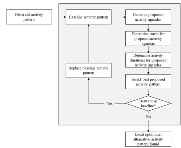
Figure 1 shows the steps within each iteration of the algorithm. For the first iteration, the 4
observed activity pattern serves as the baseline. The final activity pattern output from the
5
procedure is the alternative activity pattern. During each iteration of the hill-climbing algorithm, 6
we generate and propose numerous activity patterns, called proposed activity patterns. Lastly, 7
within these proposed activity patterns, an activity agenda consists of a set of consecutive 8
episodes, e.g. home-work-home-shop-home. This activity agenda does not provide information 9
about the timing, duration, or location of episodes, or any information about travel. 10
11
12
FIGURE 1 Alternative activity pattern generation procedure. 13
14
Generate proposed activity agendas 15
Within each iteration, the agenda of the baseline pattern serves as a skeleton. We generate every 16
unique proposed agenda that we can possibly create by applying the single elementary operations 17
to the baseline agendas. The number of proposed agendas generated in this step depends 18
primarily on the number of episodes in the observed activity pattern and the number of different 19
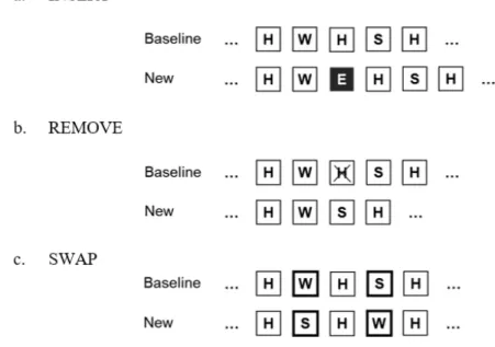
activity types. Figure 2 illustrates the elementary operations used to modify the baseline agenda. 20
These are the same elementary operations used by (22). 21
First, an attempt is made to insert a new episode between two episodes in the baseline 22
agenda (Figure 2a). This operation occurs with every activity type between every pair of 23
consecutive episodes in the baseline agenda. To preserve the “home” episodes as the anchors of 24
the daily agendas, new episodes are not inserted at the beginning or end of the agenda. If the 25
inserted episode is different in type from both the preceding and subsequent adjacent episodes in 1
the agenda, a new agenda is created. Otherwise, the procedure continues on to the next potential 2
slot or activity type. 3
Next, an attempt is made to remove a single episode at a time (Figure 2b), for every 4
episode in the baseline agenda. If the episode is not an overnight “home” episode, it is removed 5
and a new agenda is created. Otherwise, the procedure moves on to the next episode in the 6
agenda. Following the episode removal, if two consecutive episodes are of the same type, one of 7
them is removed. 8
Finally, two episodes in the baseline agenda are swapped if neither is an overnight 9
“home” episode (Figure 2c). This operation is attempted for every possible episode pair 10
combination in the agenda. By allowing this swapping operation, proposed activity patterns with 11
higher total utility can be generated. However, these patterns will likely also bear less 12
resemblance to the individual’s observed activity pattern. Whether or not swapping generates 13
reasonable changes in general requires further testing. For our example application in the next 14
section, we do not apply the swapping operation. 15
16
17 18
FIGURE 2 Example of the INSERT, REMOVE, and SWAP operations. 19
20
Determine travel for proposed activity agendas 21
This step determines the mode for every trip in every agenda using the principle of utility 22
maximization. First, each proposed agenda is aligned with the observed agenda and the closest 23
episodes of the same type within the same day are paired across the two agendas. Note that this 24
comparison is with the original, observed agenda, which is generally different from the baseline 25
agenda after the first iteration. Typically, episodes that have undergone the “insert” or “remove” 26
operations cannot be paired, because they do not have a corresponding episode in the observed 27
pattern or proposed agendas, respectively. For paired episodes, the activity location remains the 28
same. For unpaired episodes with multiple possible activity locations (e.g. if the user could 29
complete a shopping activity at similar stores in different locations), we take a myopic approach. 30
Specifically, trips are evaluated sequentially and the mode choice becomes a joint mode-31
destination choice, because each trip entails the choice between all possible modes to all possible 32
activity locations for the given activity type. The choice of mode-destination for the current trip 33
might have adverse effects on downstream mode-destination choices; however, we do not 1
account for these effects at present. A more nuanced method for selecting activity locations is 2
part of the ongoing work. 3
For a given origin-destination pair and mode 𝑚𝑚, we assume that the utility of a trip 𝑉𝑉𝑡𝑡𝑡𝑡𝑡𝑡𝑡𝑡 4
is a function of the travel time and travel cost: 5 6 𝑉𝑉𝑡𝑡𝑡𝑡𝑡𝑡𝑡𝑡 = 𝛽𝛽𝑚𝑚+ 𝛽𝛽𝑚𝑚,𝑇𝑇 ⋅ 𝑇𝑇𝑚𝑚+ 𝛽𝛽𝑚𝑚,𝐶𝐶⋅ 𝐶𝐶𝑚𝑚 (1), 7 8 where: 9
• 𝛽𝛽𝑚𝑚 is an alternative specific constant for mode 𝑚𝑚;
10
• 𝛽𝛽𝑚𝑚,𝑇𝑇 is the parameter for travel time by mode 𝑚𝑚;
11
• 𝑇𝑇𝑚𝑚 is the travel time by mode 𝑚𝑚;
12
• 𝛽𝛽𝑚𝑚,𝐶𝐶 is the parameter for travel cost by mode 𝑚𝑚; and
13
• 𝐶𝐶𝑚𝑚 is the travel cost by mode 𝑚𝑚.
14 15
The parameters can be varied for this utility function to generate a set of different activity 16
patterns, or the parameters can be estimated from a pre-survey. In addition to the utility of the 17
trip itself, the selection of mode should account for the opportunity cost of travel time, i.e., time 18
that could be spent productively on other activities. For example, if it takes a person 20 minutes 19
to drive home and 60 minutes to walk home from work, the drive option will provide him with 20
an additional 40 minutes to spend at home or to carry out another activity later on, from which he 21
can derive additional utility. In other words, the duration of the trip affects utility outside of the 22
trip itself. However, the selection of modes should account for this opportunity cost. Therefore, 23
we estimate the magnitude of the opportunity cost for a trip 𝑂𝑂𝐶𝐶 as: 24 25 𝑂𝑂𝐶𝐶 = −𝑉𝑉𝑎𝑎𝑎𝑎𝑎𝑎𝑎𝑎𝑎𝑎𝑎𝑎𝑎𝑎𝑎𝑎,𝑎𝑎𝑡𝑡𝑎𝑎𝑎𝑎𝑡𝑡 𝐷𝐷 ⋅ 𝑇𝑇𝑚𝑚 (2), 26 27 where: 28
• 𝑉𝑉𝑎𝑎𝑎𝑎𝑡𝑡𝑡𝑡𝑎𝑎𝑡𝑡𝑡𝑡𝑎𝑎,𝑡𝑡𝑡𝑡𝑡𝑡𝑎𝑎𝑡𝑡 is the total utility from all episodes in the observed activity pattern; and
29
• 𝐷𝐷 is the total duration spent on activities in the observed activity pattern. 30
31
The procedure of assigning utility to activities follows in the next section. For each trip, the 32
selected mode and destination, if applicable, are that which yield the maximum total utility, i.e. the 33
minimum sum of trip disutility and opportunity cost of travel time. 34
35
Determine activity durations for proposed activity agendas 36
With travel determined, we now determine the duration of each episode in each activity agenda 37
such that the total utility of each agenda is maximized. We assume that the utility of an activity 𝑎𝑎 38
is a function of the duration of the activity 𝐷𝐷𝑎𝑎: 39
40
𝑉𝑉𝑎𝑎𝑎𝑎𝑡𝑡𝑡𝑡𝑎𝑎𝑡𝑡𝑡𝑡𝑎𝑎 = 𝛽𝛽𝑎𝑎⋅ ln (𝛼𝛼𝑎𝑎⋅ 𝐷𝐷𝑎𝑎) (3).
41 42
Here 𝛽𝛽𝑎𝑎 and 𝛼𝛼𝑎𝑎 are scale and shape parameters, respectively, for the utility of activity type 𝑎𝑎. 43
This formulation of utility follows the method that Charypar and Nagel applied to MATSim (20). 44
Again, we can derive or estimate the parameters such that the observed activity pattern is optimal 45
without system changes, or we can vary them to generate a set of different activity patterns. For 46
positive parameters, the utility function is monotonically increasing with duration but 1
diminishing at the margin. The diminishing marginal effect can be interpreted as fatigue, 2
boredom, or other forms of efficiency loss as the duration of an activity increases. For some 3
activities in which utility is not necessarily derived intrinsically, such as work or household 4
chores, equation (3) models the extrinsic value of the activity, such as a salary or a clean house. 5
In this framework, the scheduling process is activity-driven, because travel only occurs when the 6
utility derived from an activity outweighs the disutility of travelling there. Furthermore, if we use 7
reasonable values for the 𝛽𝛽𝑎𝑎 and 𝛼𝛼𝑎𝑎 parameters, the principle of utility-maximization ensures a 8
balanced composition of activities, since the diminishing marginal utility, i.e. boredom or fatigue, 9
encourages individuals switch to activities that are more pressing or rewarding. We should also 10
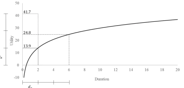
note that because the utility function (3) is non-linear, calculating utility based on duration per 11
episode versus per day or per week will yield different results (Figure 3). Here, three short 12
episodes, each with duration 𝑑𝑑𝑎𝑎, yield a total 41.7 utility units if calculated per episode. 13
However, the same three episodes yield only 24.8 utility units if the episode durations 14
accumulate over the analysis period. 15
16
17
FIGURE 3 Illustration of activity utility discrepancy for different utility accumulation 18
methods. 19
20
Calculating utility on a per episode basis generally results in more frequent short 21
episodes, because the marginal utility is higher for short episodes. On the other hand, calculating 22
utility on a per week basis results in fewer long episodes in order to minimize the disutility of 23
travel. We handle this discrepancy by distinguishing between mandatory/maintenance activities 24
and discretionary activities. In particular, we accumulate activity durations over the multi-day 25
analysis period for mandatory and maintenance activities, such as work, shop, and personal 26
errands, while we use daily accumulation for discretionary activities, such as social and 27
recreational. 28
Beyond the utility of the activity itself, proposed episodes are penalized for changing the 29
individual’s schedule, i.e. the observed activity pattern. In principle, this is similar to the 30
disutility of change used by (17). However Joh et al. apply the change to the operation itself, 31
whereas our disutility of change is a function of differences in episode start times between 32
episodes in the observed pattern and the new pattern. Only proposed episodes that successfully 33
pair with episodes in the observed agenda will produce this disutility of change. In other words, 1
newly inserted episodes and episodes that shifted to different days do not have an associated 2
disutility of change. For an episode of activity type 𝑎𝑎, equation (4) gives the disutility of change, 3 𝑉𝑉𝑎𝑎ℎ𝑎𝑎𝑎𝑎𝑎𝑎𝑎𝑎: 4 5 𝑉𝑉𝑎𝑎ℎ𝑎𝑎𝑎𝑎𝑎𝑎𝑎𝑎 = −𝑖𝑖𝑓𝑓𝑎𝑎⋅ �𝑡𝑡𝑠𝑠𝑡𝑡𝑎𝑎𝑡𝑡𝑡𝑡,𝑎𝑎𝑎𝑎𝑛𝑛− 𝑡𝑡𝑠𝑠𝑡𝑡𝑎𝑎𝑡𝑡𝑡𝑡,𝑡𝑡𝑜𝑜𝑠𝑠�2 (4). 6 7 where: 8
• 𝑖𝑖𝑎𝑎 is a parameter representing the inertia of activity type 𝑎𝑎;
9
• 𝑓𝑓 is the flexibility of the individual; 10
• 𝑡𝑡𝑠𝑠𝑡𝑡𝑎𝑎𝑡𝑡𝑡𝑡,𝑎𝑎𝑎𝑎𝑛𝑛 is the start time of the episode in the proposed pattern; and
11
• 𝑡𝑡𝑠𝑠𝑡𝑡𝑎𝑎𝑡𝑡𝑡𝑡,𝑡𝑡𝑜𝑜𝑠𝑠 is the start time of the episode in the observed activity pattern.
12 13
Intuitively, activity types that are more difficult to move temporally have higher inertia 14
and produce greater penalties when their start times have to change. On the other hand, flexible 15
individuals experience lower penalties for changes overall. Similar to other parameters in this 16
framework, the activity-specific inertia and flexibility parameters can be varied to generate 17
different activity pattern alternatives, or they can be derived from a pre-survey or a participant’s 18
observed pattern. As part of our ongoing work, we are testing different functional forms; the 19
current formulation is only an a priori hypothesis of how we penalize change. However, 20
validating these formulations as well as the parameters is challenging, and the methods to do so 21
empirically are not obvious. 22
With all travel already fixed, the duration of each episode can be determined by 23
maximizing the utility of the proposed pattern. The optimization problem is formulated as: 24 25 maxd �� 𝑉𝑉𝑎𝑎𝑎𝑎𝑡𝑡𝑡𝑡𝑎𝑎𝑡𝑡𝑡𝑡𝑎𝑎+ � 𝑉𝑉𝑎𝑎ℎ𝑎𝑎𝑎𝑎𝑎𝑎𝑎𝑎� = � 𝛽𝛽𝑎𝑎⋅ ln(𝛼𝛼𝑎𝑎⋅ 𝐷𝐷𝑎𝑎) 𝐴𝐴 26 + ∑ −𝑡𝑡𝑎𝑎,𝑒𝑒𝑛𝑛𝑒𝑒𝑛𝑛′ 𝑓𝑓 ⋅ �𝑡𝑡𝑠𝑠𝑡𝑡𝑎𝑎𝑡𝑡𝑡𝑡,𝑎𝑎𝑎𝑎𝑛𝑛,𝑎𝑎𝑛𝑛𝑒𝑒𝑛𝑛′ − 𝑡𝑡𝑠𝑠𝑡𝑡𝑎𝑎𝑡𝑡𝑡𝑡,𝑡𝑡𝑜𝑜𝑠𝑠,𝑎𝑎𝑛𝑛𝑒𝑒𝑛𝑛′ � 2 𝐸𝐸𝑛𝑛𝑒𝑒𝑛𝑛′ 𝑎𝑎𝑛𝑛𝑒𝑒𝑛𝑛′ (5), 27 𝑠𝑠. 𝑡𝑡. ∑𝑅𝑅𝑡𝑡𝑛𝑛𝑒𝑒𝑛𝑛𝑛𝑛𝑒𝑒𝑛𝑛𝑇𝑇𝑡𝑡𝑛𝑛𝑒𝑒𝑛𝑛 + ∑𝑎𝑎𝐸𝐸𝑛𝑛𝑒𝑒𝑛𝑛𝑛𝑛𝑒𝑒𝑛𝑛𝑑𝑑𝑎𝑎𝑛𝑛𝑒𝑒𝑛𝑛− ∑ 𝑇𝑇𝑡𝑡𝑡𝑡𝑜𝑜𝑜𝑜 𝑅𝑅𝑡𝑡𝑜𝑜𝑜𝑜 𝑡𝑡𝑡𝑡𝑜𝑜𝑜𝑜 − ∑ 𝑑𝑑𝑎𝑎𝑡𝑡𝑜𝑜𝑜𝑜 𝐸𝐸𝑡𝑡𝑜𝑜𝑜𝑜 𝑎𝑎𝑡𝑡𝑜𝑜𝑜𝑜 = 0 28 29 where: 30
• 𝑑𝑑𝑎𝑎 is the duration of an episode 𝑒𝑒; 31
• 𝐷𝐷𝑎𝑎 is the sum of durations of episodes 𝑒𝑒 of activity type 𝑎𝑎 that accumulate by day or by 32
analysis period; 33
• 𝐴𝐴 is the set of all activity types 𝑎𝑎; 34
• 𝐸𝐸 is the set of episodes 𝑒𝑒 within the day being optimized; 35
• 𝐸𝐸′ is the set of episodes 𝑒𝑒′ that pair with episodes in the observed pattern within the day 36
being optimized, i.e. a subset of 𝐸𝐸; 37
• 𝑅𝑅 is the set of all trips 𝑟𝑟 within the day being optimized; 38
• 𝑛𝑛𝑒𝑒𝑒𝑒 in the subscript denotes that the value is from the new pattern; 39
• 𝑜𝑜𝑜𝑜𝑠𝑠 in the subscript denotes that the value is from the observed pattern; and 40
• 𝑡𝑡𝑠𝑠𝑡𝑡𝑎𝑎𝑡𝑡𝑡𝑡,𝑎𝑎𝑎𝑎𝑛𝑛,𝑎𝑎 is the start time of episode 𝑒𝑒 in the new activity pattern, i.e. 41
𝑡𝑡𝑠𝑠𝑡𝑡𝑎𝑎𝑡𝑡𝑡𝑡,𝑎𝑎𝑎𝑎𝑛𝑛,𝑎𝑎 = 0 for 𝑒𝑒 = 0, and 𝑡𝑡𝑠𝑠𝑡𝑡𝑎𝑎𝑡𝑡𝑡𝑡,𝑎𝑎𝑎𝑎𝑛𝑛,𝑎𝑎 = 𝑡𝑡𝑠𝑠𝑡𝑡𝑎𝑎𝑡𝑡𝑡𝑡,𝑎𝑎𝑎𝑎𝑛𝑛,𝑎𝑎−1+ 𝑑𝑑𝑎𝑎−1 for 𝑒𝑒 > 0.
42 43
Because utility for non-discretionary activities accumulates beyond a single day, the 1
episode durations within the day depend on episode durations on other days within the analysis 2
period, as these episode durations undergo optimization. This procedure can be interpreted as the 3
individual’s knowledge of the past and plan for the future. The individual currently bases his 4
plan for the future on his observed pattern. Consider, for example, work durations over a week. 5
On Monday a person knows how much he should work that week (reflected by the 𝛽𝛽-parameter 6
for work). He also has a plan for how much he will work on each day and will try to work a 7
certain number of hours on Monday, so that the total hours add up to the planned hours. 8
However, if he inserts an additional activity on Monday, he will work fewer hours on Monday 9
than in the observed pattern. Subsequently, on Tuesday, he will know he worked too little the 10
previous day and will try to compensate, so that the total hours once again add up. 11
12
Select best alternative activity pattern 13
Finally, the total utility of each proposed activity pattern is evaluated: 14
15
𝑉𝑉𝑡𝑡𝑡𝑡𝑡𝑡𝑎𝑎𝑡𝑡 = ∑ 𝑉𝑉𝑡𝑡𝑡𝑡𝑡𝑡𝑡𝑡+ ∑ 𝑉𝑉𝑎𝑎𝑎𝑎𝑡𝑡𝑡𝑡𝑎𝑎𝑡𝑡𝑡𝑡𝑎𝑎+ ∑ 𝑉𝑉𝑎𝑎ℎ𝑎𝑎𝑎𝑎𝑎𝑎𝑎𝑎 (6)
16 17
Note that we do not include the opportunity cost of travel time here, because it is already 18
accounted for in 𝑉𝑉𝑎𝑎𝑎𝑎𝑡𝑡𝑡𝑡𝑎𝑎𝑡𝑡𝑡𝑡𝑎𝑎. 19
If the best of the proposed activity patterns has a higher utility than the baseline pattern, 20
another iteration of the algorithm runs using the agenda of the best proposed pattern as the new 21
baseline. Otherwise, the current baseline is selected as the best pattern for the given input 22 parameters. 23 24 PROOF-OF-CONCEPT APPLICATIONS 25
We tested this proposed procedure for alternative activity pattern generation on a dataset from a 26
multi-day activity survey conducted in Singapore in 2013 (1). This smartphone-based survey 27
contains detailed travel, activity, and location information from consecutive weekdays, e.g. 28
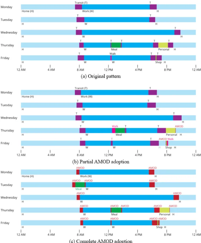
Monday through Friday in the same week.Figure 4a shows one participant’s observed weekly 29
activity pattern. In a complete SP experiment, we would collect multi-day or multi-week activity 30
diaries for each respondent to establish a baseline. The respondent would also complete a pre-31
survey, which along with the observed activity patterns inform his preference parameters. We 32
would then change system variables to reflect a hypothetical scenario, e.g. increased/decreased 33
travel times by certain modes, restricted mode choices, etc. Then using the proposed method and 34
different sets of input parameter, we generate different alternative activity patterns that form a 35
choice set. In general, input parameters can be derived from the observed patterns or the 36
respondent’s pre-survey. However, for parameters that will be used to estimate a model, the input 37
parameters must be generated randomly to avoid endogeneity. 38
Here, we consider a hypothetical scenario in which on-demand AV service, Automated 39
Mobility On-Demand (AMOD), is introduced, and examine examples of alternative activity 40
patterns generated for the abovementioned survey participant. Given that such a service does not 41
yet exist, it is difficult to judge the method’s predictive accuracy. However, our objective is only 42
to generate numerous feasible alternatives that form a choice set for respondents to choose 43
between, thus perfect predictions of actual responses are not necessary at this stage. For the 44
purposes of this proof-of-concept demonstration, we assume that AMOD travel times are the 45
same as travel times by automobile at twice the cost of completing the same trip by transit. 46
Depending on the individual’s preferences, adopting AMOD for one or more trips might improve 47
the overall utility of their activity pattern. We select the preference parameters for this 1
demonstration (Table 1) by assuming that the mode-specific constants, 𝛽𝛽𝑚𝑚, are 0 for all modes 2
and that other preference parameters associated with travel and change fall within a reasonable 3
range. These a priori values were assumed for proof-of-concept demonstration purposes. A 4
different set of parameters would generate different alternative patterns. Lastly, we derive the 5
preference parameters associated with activities from the observed activity pattern, such that 6
activity choices would remain similar if there were no changes to the system. 7
8
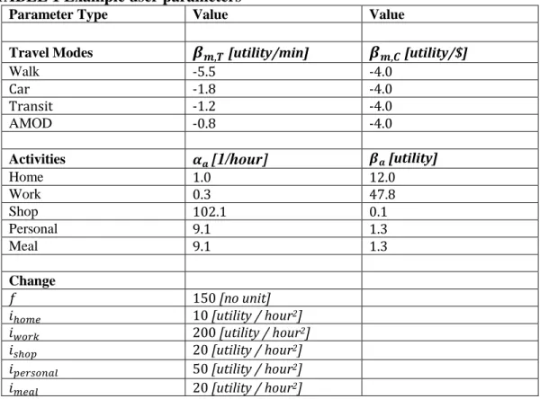
TABLE 1 Example user parameters 9
Parameter Type Value Value
Travel Modes 𝜷𝜷𝒎𝒎,𝑻𝑻 [utility/min] 𝜷𝜷𝒎𝒎,𝑪𝑪 [utility/$]
Walk -5.5 -4.0
Car -1.8 -4.0
Transit -1.2 -4.0
AMOD -0.8 -4.0
Activities 𝜶𝜶𝒂𝒂[1/hour] 𝜷𝜷𝒂𝒂 [utility]
Home 1.0 12.0 Work 0.3 47.8 Shop 102.1 0.1 Personal 9.1 1.3 Meal 9.1 1.3 Change 𝑓𝑓 150 [no unit] 𝑖𝑖ℎ𝑡𝑡𝑚𝑚𝑎𝑎 10 [utility / hour2] 𝑖𝑖𝑛𝑛𝑡𝑡𝑡𝑡𝑤𝑤 200 [utility / hour2] 𝑖𝑖𝑠𝑠ℎ𝑡𝑡𝑡𝑡 20 [utility / hour2] 𝑖𝑖𝑡𝑡𝑎𝑎𝑡𝑡𝑠𝑠𝑡𝑡𝑎𝑎𝑎𝑎𝑡𝑡 50 [utility / hour2] 𝑖𝑖𝑚𝑚𝑎𝑎𝑎𝑎𝑡𝑡 20 [utility / hour2] 10
Work, shopping, and personal errands fall into the category of mandatory/maintenance 11
activities, and thus their durations accumulate over the entire survey period for utility calculation 12
purposes. We categorize home and meal breaks as discretionary activities. Arguably, home can 13
be considered a mandatory/maintenance activity; however, because we never remove overnight 14
home episodes, the remaining home-related decisions are of a discretionary nature, e.g. how long 15
to spend at home, whether to return home between activities, or whether to extend the tour. 16
Figure 4b presents the generated alternative activity pattern. In this pattern, the survey 17
participant uses AMOD for two trips, once Thursday night on his way home from the personal 18
errand and once Friday evening for his shopping trip. The convenience of AMOD also 19
introduced a new home episode on Friday, making shopping a separate home-based tour. 20
However, as expected, the relatively high cost of the service results in limited adoption and 21
minimal impact on the observed activity pattern, with the assumed preference parameters. 22
Figure 4c presents a different final alternative activity pattern, in which we explore the 23
impact of complete AMOD adoption. We removed the walk, car, and transit mode options and 24
halved the magnitude of the AMOD parameters, i.e. 𝛽𝛽𝐴𝐴𝐴𝐴𝐴𝐴𝐷𝐷,𝑇𝑇= −0.4/𝑚𝑚𝑖𝑖𝑛𝑛 and 25
𝛽𝛽𝐴𝐴𝐴𝐴𝐴𝐴𝐷𝐷,𝐶𝐶 = −2/$. The shorter AMOD travel times allow the survey participant to leave home
later in the morning and return home earlier in the evening. For example, on Thursday he would 1
arrive home at 8:26 pm as opposed to 8:55 pm. At the same time, he would add a meal episode 2
on Tuesday, and available work time increases from 47.8 hours to 48.6 hours. 3
These examples also highlight the limitations of the proposed method in its current state. 4
The sequential, iterative approach does not account for travel times that vary according to the 5
time of day; thus, we base all travel times in the alternative patterns on evening peak travel 6
conditions. Not only does this potentially affect the selection of mode, it also inaccurately 7
determines the time available for activities. Similarly, activity demands are constant throughout 8
the day, a potentially unrealistic property that the additional hour-long meal break before 8 am on 9
Tuesday in the second alternative pattern illustrates. 10
1
FIGURE 4 An individual’s observed weekly activity pattern (a), example alternative 2
activity pattern with partial AMOD adoption (b) and complete AMOD adoption (c). 3
CONCLUSION AND FUTURE DIRECTION 1
We have presented a new method for generating activity-driven, multi-day alternative activity 2
patterns, designed for use in stated preference surveys. This method generates alternatives using 3
a local optimization algorithm that searches for the best response to a system change that is 4
similar to the survey participant’s observed patterns. The alternative patterns also allow us to 5
explore the propagation of indirect effects resulting from the participant’s direct response. As a 6
proof-of-concept, we applied the method to data from a multi-day activity-travel survey in 7
Singapore and considered the hypothetical implementation of an on-demand AV service. The 8
demonstration showed promising results with the algorithm exhibiting overall desirable behavior 9
with reasonable responses. However, the examples highlight the method’s current limitations, 10
namely inflexibility vis-à-vis activity demand and travel times depending on the time of day. In 11
our continued work, we plan to address these limitations as well as to allow for substitution of 12
activities within activity types, e.g. the substitution of office work with teleworking. 13
Incorporating additional ways to constrain alternatives to the observed pattern might also enable 14
more nuance in the generated activity patterns. Currently the measure of change is considered 15
with the difference in start times of activities but the change in the total number of activities is 16
another candidate to impose further constraints. 17
As we improve the method, we will test the generated activity patterns on respondents to 18
calibrate and ensure that we are generating relevant alternatives. We will soon employ the 19
proposed method in two activity-based experiments focusing on AMOD adoption and carbon 20
emissions feedback. For the first experiment, a stated preference survey, we will test how to align 21
the experimental treatments, namely the AMOD services, with the activity generation procedure 22
we proposed. For instance, instead of presenting the participants with the full range of AMOD 23
adoption possibilities shown in the proof-of-concept above, we can first gather the participants’ 24
stated preferences for their level of adoption of AMOD services or subscription programs. Then, 25
we can use their adoption preferences to tailor the set of alternative activity patterns that we 26
present to the participants in the second part of the stated preference survey and evaluate whether 27
the participants accept the impact of the AMOD treatment on their overall activity patterns. The 28
proposed method can also be developed into a travel-activity planning advisory application that 29
automatically generates feedback and personalized advice based on users’ stated or revealed 30
preferences. In the second experiment, we will test the effectiveness of smartphone-based 31
activity-travel and carbon emissions feedback delivery for encouraging sustainable behavior 32
change. The algorithm’s multi-day pattern generation capability can support recommendations 33
for blended travel mode choices over extended study periods. Additionally, by accounting for the 34
multidimensional impacts of changing activities and travel in realistic alternative patterns, this 35
method can help test the effectiveness of an assisted behavioral planning program. 36
37
ACKNOWLEDGEMENTS 38
The MIT Energy Initiative (MITEI) Seed Grant Fund and the National Research Foundation 39
Singapore, through the FM IRG research group at the Singapore-MIT Alliance for Research and 40
Technology, supported this research. 41
REFERENCES 1
1. Cottrill, C., F. Pereira, F. Zhao, I. Dias, H. B. Lim, M. Ben-Akiva, and C. Zegras, 2
Future Mobility Survey: Experience in Developing a Smart-Phone-Based Travel 3
Survey in Singapore, Transportation Research Record: Journal of the 4
Transportation Research Board, issue 2354, pp. 59-67, 2013.
5
2. Bowman, John L., and Moshe Ben-Akiva. Activity based travel forecasting, 6
Activity based travel forecasting conference, New Orleans, June 1996.
7
3. Axhausen, Kay W., and Tommy Gärling. Activity-based Approaches to Travel 8
Analysis: Conceptual Frameworks, Models, and Research Problems. Transport 9
Reviews, 12, 1992, pp. 323–341, https://doi.org/10.1080/01441649208716826
10
4. Recker, Wilfred W. The household activity pattern problem: General formulation 11
and solution. Transportation Research Part B: Methodological, Volume 29, Issue 12
1, 1995, pp. 61-77, http://dx.doi.org/10.1016/0191-2615(94)00023-S. 13
5. Kitamura, Ryuichi, and Satoshi Fujii. Two Computational Process Models of 14
Activity-Travel Behavior. Theoretical Foundations of Travel Choice Modeling, 15
1998, pp. 251–279 16
6. Lu, Yang, Muhammad Adnan, Kakali Basak, Francisco Câmara Pereira, Carlos 17
Carrion, Vahid Hamishagi Saber, Harish Loganathan, and Moshe E. Ben-Akiva. 18
SimMobility mid-term simulator: A state of the art integrated agent based demand 19
and supply model. Transportation Research Board, Washington DC, 2015. 20
7. Miller, Eric, and Matthew Roorda. Prototype model of household activity-travel 21
scheduling. Transportation Research Record: Journal of the Transportation 22
Research Board 1831, 2003, pp. 114-121.
23
8. Roorda, Matthew J., Eric J. Miller, and Khandker M.N. Habib, Validation of 24
TASHA: A 24-H Activity Scheduling Microsimulation Model, Transportation 25
Research Part A: Policy and Practice, Volume 42, Issue 2, 2008, pp. 360–75.
26
doi:10.1016/j.tra.2007.10.004. 27
9. Arentze, Theo, and Harry Timmermans, Albatross: A Learning Based 28
Transportation Oriented Simulation System, Eirass Eindhoven, 2000.
29
10. Pinjari, Abdul Rawoof, and Chandra R. Bhat. Activity-Based Travel Demand 30
Analysis, A Handbook of Transport Economics 10, 2011, pp. 213–248. 31
11. RDC, Activity-based modeling system for travel demand forecasting, 32
Metropolitan Washington Council of Governments, US Department of 33
Transportation, US Environmental Protection Agency, Washington DC, 1995. 34
12. Doherty, Sean, Martin Lee-Gosselin, Kyle Burns, and Jean Andrey, Household 35
Activity Rescheduling in Response to Automobile Reduction Scenarios, 36
Transportation Research Record: Journal of the Transportation Research Board,
37
no. 1807, 2002, pp. 174–181. 38
13. Doherty, Sean T., and Eric J. Miller, A Computerized Household Activity 39
Scheduling Survey, Transportation, Volume 27, Issue 1, 2000, pp. 75–97. 40
14. Lee, Ming S., and Michael G. McNally, On the structure of weekly activity/travel 41
patterns, Transportation Research Part A: Policy and Practice, Volume 37, Issue 42
10, 2003, pp. 823-839. 43
15. Auld, Joshua, Martina Z. Frignani, Chad Williams, and Abolfazl Kouros 44
Mohammadian, Results of the UTRACS Internet-Based Prompted Recall GPS 45
Activity-Travel Survey for the Chicago Region, 12th World Conference in
46
Transportation Research, Lisbon, Portugal, 2010.
16. Timmermans, Harry, Theo Arentze, and Chang-Hyeon Joh, Modeling effects of 1
anticipated time pressure on execution of activity programs, Transportation 2
Research Record: Journal of the Transportation Research Board 1752, 2001, pp.
3
8-15, doi:10.1016/j.tra.2007.10.004. 4
17. Joh, Chang-Hyeon, Theo Arentze, and Harry Timmermans, Modeling 5
Individuals’ Activity-Travel Rescheduling Heuristics: Theory and Numerical 6
Experiments, Transportation Research Record: Journal of the Transportation 7
Research Board, no. 1807, 2002, pp. 16–25.
8
18. Joh, Chang-Hyeon, T. A. Arentze, and H. J. P. Timmermans, Estimating Non-9
Linear Utility Functions of Time Use in the Context of an Activity Schedule 10
Adaptation Model, 10th International Conference on Travel Behavior Research,
11
2003. 12
19. Nagel, Kai, Kay W. Axhausen, Benjamin Kickhöfer, and Andreas Horni, 13
Research Avenues, In The Multi-Agent Transport Simulation MATSim (Andreas 14
Horni, Kai Nagel, and Kay W. Axhausen, ed.), Ubiquity Press, 2016, pp. 533–42, 15
doi:10.5334/baw.97. 16
20. Arentze, T. A., Claudia Pelizaro, and H. J. P. Timmermans. Implementation of a 17
Model of Dynamic Activity-Travel Rescheduling Decisions: An Agent-Based 18
Micro-Simulation Framework. In Proceedings of the Computers in Urban 19
Planning and Urban Management Conference, Volume 48, 2005.
20
21. Nagel, Kai, Benjamin Kickhöfer, Andreas Horni, and David Charypar, A Closer 21
Look at Scoring. In The Multi-Agent Transport Simulation MATSim (Andreas 22
Horni, Kai Nagel, and Kay W. Axhausen, ed.), Ubiquity Press, 2016, pp. 23– 23
34.doi:10.5334/baw.3. 24
22. Balac, Milos, and Kay W. Axhausen Activity rescheduling within a multi-agent 25
transport simulation framework (MATSim), Transportation Research Board, 26
Washington DC, 2017. 27
View publication stats View publication stats