HAL Id: hal-01104035
https://hal.archives-ouvertes.fr/hal-01104035
Preprint submitted on 15 Jan 2015HAL is a multi-disciplinary open access
archive for the deposit and dissemination of sci-entific research documents, whether they are pub-lished or not. The documents may come from teaching and research institutions in France or abroad, or from public or private research centers.
L’archive ouverte pluridisciplinaire HAL, est destinée au dépôt et à la diffusion de documents scientifiques de niveau recherche, publiés ou non, émanant des établissements d’enseignement et de recherche français ou étrangers, des laboratoires publics ou privés.
EcoAdapt Working Paper Series N°2: iModeler manual:
a quick guide for fuzzy cognitive modelling
Grégoire Leclerc
To cite this version:
Grégoire Leclerc. EcoAdapt Working Paper Series N°2: iModeler manual: a quick guide for fuzzy cognitive modelling. 2014. �hal-01104035�
EcoAdapt Working Paper Series N°2
Adaptation to climate change for local development
iModeler manual: a quick guide
for fuzzy cognitive modelling
Grégoire Leclerc, CIRAD, [email protected]
Authorship
Lead author: Grégoire Leclerc. Email: [email protected]. Developed and tested the FCM
models and wrote the working paper.
Contributors
Reviewer: Raffaele Vignola. Email: [email protected]. Provided useful comments on the text. Contributor: Kai Neuman. Email: [email protected]. Provided timely feedback on technical
questions about iModeler. Some of the material of iModeler guides have been used or adapted for this document.
Collaborators
Collaborator: Ralf Schillinger. Email: [email protected]. Provided feedback on FCM modelling.
Collaborator: Mareen Cristine Hüls. Email: [email protected]. Provided feedback on
FCM modelling and did early tests for Jujuy.
Versions
Version 1: 14/1/2014. Deliverable 3.3 submitted to the European Union.
Version 2: 11/11/2014. Version not yet validated by partners and corresponding to iModeler version
Table of content
Abstract ...4
1. Introduction ...5
2. Background ...6
3. On the use of [complex] quantitative models for decision making ...7
4. Basic principles of FCM ...8
4.1. Strengths and weaknesses of FCM ...9
5. iModeler qualitative and quantitative FCMs ... 11
6. Qualitative modelling ... 12
6.1. Refining factors and influences ... 17
6.2. Examine model and results (iModeler) ... 26
6.3. Documenting and versioning ... 35
7. Quantitative modeling ... 38
8. Implemented qualitative models ... 46
8.1. Jujuy model forest FCM ... 47
8.2. Chiquitano Model Forest FCM ... 55
8.3. Araucas del Alto Malleco Model Forest FCM ... 57
9. Using FCM models for Scenario and Simulation (S&S) ... 59
10. Concluding remarks and next steps ... 63
Acknowledgements ... 64
Abstract
We introduce Fuzzy Cognitive Modelling (FCM) and provide step by step guidance and tips for using iModeler (both qualitative and quantitative approaches), the use of FCM in EcoAdapt Story and Simulation (S&S) approach based on Structured Decision Making, and briefly describe the FCM models being developed in the three study sites. This version correspond to iModeler version 4 (January 2004).
1. Introduction
Cognitive maps are qualitative graphical models of a system, consisting of a set variables linked together by causal relationships1. A cognitive map can be made of almost any system or problem,
and therefore particularly useful for creating models based on people’s knowledge (experts and lay people). As a tool to express people’s mental models, it is useful as brainstorming tool, an
alternative to other “discussion support tools” such as the mind map (associative relationship among ideas). A form of cognitive maps, the concept map2 (Novak, 1990), typically allow to build
interconnected build propositions, i.e. concept-relation-concept (e.g. “farmer manages its farm”) from people’s discourses, and as such can be built quickly without any technical skills, and is readily understandable by a technical or non-technical audience. Cognitive maps are important in decision-making since 1) they help raise self-awareness of complexities 2) help communication by decision-making tacit knowledge explicit 3) they reveal how individual perceptions of reality shape choices 4) they make explicit critical choices parameters and trade-offs, encouraging negotiation and promoting win-win solutions.
Concept maps, like influence diagrams or mind maps, are essentially semantic or graphic, therefore they are not meant for numerical processing e.g. for scenario analysis, for assessing the sensitivity of parameters, or for impact assessment. Causal mapping like influence diagrams or binary cognitive maps (or bayes nets which allows to specify joint probabilities) are a step further in a more
quantitative (yet fuzzy) assessment of complex systems. Kosko (1986) modified binary cognitive maps (Axelrod, 1976) by applying fuzzy causal functions, i.e. assigning real numbers in [−1, 1] to the
relationship between factors, thus the term fuzzy cognitive map (FCM) (Özesmi and Özezmi, 2004). Kosko (1987) was also the first to compute the outcome of a FCM, or the FCM inference, as well as to model the effect of different policy options using neural networks. Modern FCM combine aspects of fuzzy logic, neural networks, semantic networks, expert systems, and nonlinear dynamical systems. FCMs are increasingly used to address a great diversity of problems, from knowledge representation, fuzzy control, engineering, approximate reasoning, strategic planning, management medical decision making, game theory, and data mining analysis. Closer to our research interests, FCM have been used for environmental policy (Kontogianni et al, 2012), developing freshwater future scenarios in Europe (VanVliet et al, 2010), analyzing deforestation in the Brazilian amazon (Kok, 2009), Ecosystem conservation and ecological modeling (Ozesmi and Ozesmi, 2003; 2004).
Given the context of our intervention (scarcity of data, multi-stakeholder decision-making, science-society processes) we judged that FCM was promising for developing, jointly with stakeholders, scenarios and alternatives and evaluate their consequences3. However going from a positivist
paradigm (e.g. quantitative models) to a constructivist one (e.g. qualitative or semi quantitative models) is not obvious, as those of us trained with a positivist mindset may have to be convinced of the benefits of a more “fuzzy” approach to modeling. Therefore, the approach is similar to grounded theory or qualitative social research, where “reality” is context-dependent scenarios of possible developments are uncertain.
1 Cognitive maps are directed graphs, or digraphs, and thus they have their historical origins in graph theory,
which started with Euler in 1736 (Biggs et al., 1976).
2 See e.g. http://cmap.ihmc.us/
This section is based on our efforts in implementing FCM in EcoAdapt sites, to provide methods, best practices and tips, highlighting their strengths and weaknesses. It has benefited from feedback from CSO staff during on-site training in FCM modelling by CIRAD in Jujuy and Bolivia in October and November 2013.
2. Background
Are decision-support systems (DSS) based on hard data and models useful for decision-making? A brief look at adoption of decision support systems (which rely on data and models) in management reveals a series of limitations and pitfalls which favors the use of more adequate, flexible and user-friendly tools to help decision-making. The main limitations of DSS are:
• The required level of user’s technological knowledge is often high.
• Many factors (if not most) are hard to quantify, and the decision-maker must use their own judgment in making the final decision. Data is often hard to collect, organize, and analyze, and one often need to rely on proxies. Data about the future is generally unavailable and ridden by uncertainties and assumptions.
• Model assumptions are often not clear for decision-makers, and often driven by the feasibility of the model given available resources.
• Model design may not respond to the needs of decision makers (which are generally not clear either).
• There is little experience in using models for decision-making, and there may be
organizational resistance for doing so. Analysis of technology adoption have helped identify critical factors, which in fact apply to many technical or social innovations (such as our use of models to support adaptation planning). The Technology Acceptance Model (TAM -Davis, 1989 - Figure 1), based on the Theory of Reasoned Action (Fishbein & Ajzen,1975), has been highly successfully applied in a broad range of contexts. The first factors to consider are the Perceived ease of use and the Perceived usefulness.
The two latter points are especially important. The ultimate goal of our models is not to mimic reality and provide solutions, but to stimulate stakeholders support for finding and implementing robust solutions. Therefore our models first have to respond to decision-makers’ needs (and help shape these needs), and have a perceived usefulness and perceived ease of use for them. In some circumstances a simple mind map (i.e. a graphical model of the system) that managers understand and that allow proper coordination may be much more useful for decision-making than a complex, numerical DSS.
3. On the use of [complex] quantitative models for decision making
Still, well embedded in today’s managers’ and policy-makers minds (and even more in natural scientists’ mind) is a positivist, engineer-like standpoint about how data and studies help decision making. Indeed in real life the same managers rely very little on “hard data” and even less on computer simulations.Let us have a look at WTO agriculture negotiations, which could well benefit from trade models. Back in 2001 during the first round of the Doha trade negotiations, while the US negotiators were testing alternatives in real-time (using the Michigan Model of World Production and Trade), most negotiators (France for instance) didn’t use models at all (e.g. econometric, computable general or partial equilibrium models, or gravity models) to assess alternatives and back-up their decisions – which does not mean that their decisions were bad. They were relying (like most of us) on their intuition and heuristics (patterns and experiences from the past); at best some may have partially relied on model results prepared by other countries (e.g. from the US)4. It is amazing that even
today, models are still marginally used for these extremely important and well framed negotiations, probably because models cannot substitute for decision-making and need to be properly understood by decision-makers: the quality of model results depend on many factors, and decision-makers need to exercise judgment on how much model results are accountable. So is it realistic to think that complex quantitative models (even simple ones, indeed!) can help small-scale, multi-stakeholders’ decision making? And more, knowing that most quantitative models are oversimplification of reality (assumptions, data restrictions, etc..)?
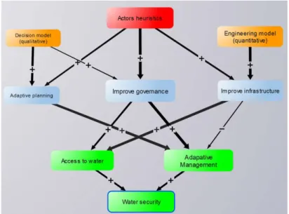
Looking at EcoAdapt approach to planning, using Structured Decision Making (Vignola and Leclerc, 2014) backed by models, one can see that quantitative models can be useful in some situations, and qualitative models in others (Figure 2).
4 After that episode France decided to develop their own model focusing on the multiple functions of
agriculture, in which CIRAD was involved. However, there is no evidence that negotiators using models were more successful than the ones that did not!
Figure 2: Hypothetical example of EcoAdapt Mean- and Ends- objectives network (see D3.1) and how actors (with their own heuristics) may reach these objectives with the help of models (quantitative or qualitative).
4. Basic principles of FCM
Altough iModeler is not a “pure” FCM, it is worthwhile to understand how FCM work, then state the differences with iModeler.
• Concepts (or “factors”): C1, C2, . . ., Cn. These represent the drivers and constraints that are considered of importance to the issue under consideration.
• State vector: A = (a1, a2, . . ., an), where ai denotes the state of the node Ci. The state vector represents the value of the concepts, usually between 0 and 1. The dynamics of the state vector is the principal output of applying a Fuzzy Cognitive Map.
• Influences: weight (usually following a Likert scale between -1 and 1) of the influence of one concept on another, i.e. how much the value of a concept increases or decreases from the influence of another concept. This is usually stated (internally to the software) as an Adjacency matrix: E = (eij), where eij is the weight of the influence CiCj.
In an FCM simulation, the value of the concepts (the state vector) changes with each time step according to the influences of other concepts: the new state vector B can be calculated by a matrix calculation, i.e. B = A×E5. This multiplication can be repeated as often as desired, which shows how
the value of concepts change over time (Figure 3). In other words, the value of a concept increases
(or decreases if influences are negative) exactly from the sum of the value of the infuences that point to it (value of concept x weight of influence).
Figure 3: hypothetical FCM showing (top) concepts C1, C2, C3 and their mutual positive and negative influences, and (bottom) the evolution of value of concepts with each iteration (source: Kok , 2009). Most FCM display a transient behavior then a stabilization of state vectors.
Few software implementation of FCM exist:
• “pure fcm”: as a asset of excel macros6, a web-based applet7, java applets8
• “hybrid FCM-System Dynamics”: iModeler.
• System dynamics (which can be used to program a FCM – e.g. Stella, Goldsim)
In the iModeler approach the concepts are meant as stocks, which means that, contrary to FCM which considers that influences have an instantaneous effect, the value of concepts change the next time step (i.e. a delay of 1 time step is applied to the influences). This is currently a trend for improving FCMs (Kok, 2009) as delays are frequent in Socio-ecosystems (e.g. time to successfully implement a policy). Also, qualitative modelling look on how a pulse (a change of value of one concept) propagates in the system, emphasizing on the strength of the while the value of the state-vector can be assessed only via quantitative modelling (section 2.6).
4.1. Strengths and weaknesses of FCM
6http://www.fcmappers.net/joomla/index.php?option=com_content&view=article&id=52&Itemid=53
(inactive since 2009)
7 (http://www.ochoadeaspuru.com/fuzcogmap/software.php (inactive since 2006, some incompatibility
problems with modern brouwsers); http://www.fcmplayground.com/ (beta)
Whenever we face a complex challenge in business, politics, society, science or in a private situation, cause and effect models help to grasp the interplay of the situation’s underlying factors. To that account Fuzzy Cognitive Maps:
• Improve system understanding
• Allow inclusion of qualitative variables (using proxies that represent an intensity). • do not need hard data
• show effects of changes in feedbacks • can include social factors
• are flexible.
The nature of adaptation to climate change in water resources, when mainstreamed in local development, is a highly complex issue whose alternatives entail a large variety of data sources, asymmetries in availability of data, precision, type of data, etc. The strongest advantage of FCMs (vs e.g. cognitive maps) is that it allows assessing the dynamics of a highly complicated (or complex) system in addition to only its structure or function. FCMs may be useful for our goal, having their weaknesses in mind is of utter importance in a participatory setting (Table 1).
Table 1 Strengths and weaknesses of FCM (Source: Author).
Strengths Weaknesses
Quick development of models Models may be inconsistent if one does not apply basic design principles
Easy integration of new factors (high level of
integration) Easy to be inconsistent in terms of units and weights (comparing non-comparable factors); reliance on experts (may exclude others)
Easy to integrate expert or local knowledge Difficult to judge accuracy of weights estimations (calibration/validation)
Helps dialogue and ownership with stakeholders;
good in a participatory process Maybe interpreted differently by various stakeholders (or some may be excluded because they do not grasp the FCMs properly); complex models may lead to non-intuitive results; yet another participatory method: possible participant fatigue Helps identify important and unimportant factors
through their impact, useful for system steering Some factors deemed important may be model artifacts Allows assessing system dynamics (and eventually
resilience e.g. short- and long-term dynamics) Sensitivity of dynamics on input parameters or weights of influences difficult to assess Possibility to model anything Models may not be able to properly describe
phenomena e.g. price formation by supply-demand, limits (thresholds, finite space, etc...) – lack of proper validation.
Flexible definition of time Meaningless definition of time, inconsistent with weight of influences; difficult to implement seasonality
Helps understanding of complex systems; overcome our mental limits and be able to grasp the interplay of more than four interdependent factors
Generates confusion before system too complex! People may think that they already know (sort of) how things work, that what they need are detailed studies or quantitative models
Provides insight on the role of key (often hidden)
feedbacks in the system. Effect of feedbacks can be highly dependent on initial conditions Can be used to improve storylines of scenarios or Can be time consuming in order to be exhaustive;
articulation of factors, feedback loops) knowledge for proper assessment of influences; possible lower involvement of laymen and free thinkers in drafting storylines
Forces to specify factors and relative strength of influences – easier link to quantitative models (I some cases FCMs can even substitute for
quantitative models); Forces to make assumptions explicit
Methods for evaluations weights not well structured; evaluations partly arbitrary (no evidence to support); risk of too much focus on numbers (steam work). (note that this has less impact when there is true co-construction of FCMs with stakeholders)
Good for understanding how to steer the system Some important factors may be the result of modelling artifacts
Reveal cognitive aspects Taking into account all perspectives can make the model overly complex
Helps develop adaptive capacity, e.g. test options ex-ante, lower the sense of gainers and losers (everyone has a role in a system), etc..
Ease of use that can lead to intention to use Available software is generally in english (iModeler has Spanish, Portuguese, German as well)
The following sections focus on methodological issues for building a meaningful FCM, and provide tips, including those specific to iModeler.
5. iModeler qualitative and quantitative FCMs
iModeler has two approaches to FCM, each of which being virtually independent. Many features apply only to qualitative modelling (e.g. insight matrix, loops, direct and indirect impacts, etc) while others apply only to Quantitative (time series, factor levels, formulas).
Therefore in iModeler the first step is to decide what kind of FCM one wants to develop, i.e. qualitative or quantitative, which depends on the goal of the model and available resources. Qualitative modelling, which is much quicker to develop than quantitative modelling, helps assess the strength of the forces that act on the system, which allow to “steer” the system (see box 1). Quantitative modelling allows assessing how factors evolve with time, i.e. their “trajectories”. Note that it is much easier to assess influences accurately than predict accurate trajectories.
Therefore if the question is “what can we do, which has the greatest impact on one or several factors?”, then qualitative modelling is useful. If the question is “how things may evolve over time?”, then quantitative modelling is required.
But there are also other factors to take into account: if the goal is to have people contribute to the model, use it (or support its use) or develop their own, if there is no data about most of the factors (and no time or money to obtain it), if there is nobody in the team that can develop equations, then qualitative FCM is the best option: it is probably better to learn how to steer the system than rely only on intuition and a limited capacity to handle many interacting factors at a time, or rely on an over simplistic quantitative model.
If you need to see how factor strength evolve with time (e.g. trends, indicators), if you need to impose limits on a given factor (e.g. height of water in a dam), need to consider thresholds, control time and units, then you will need quantitative FCM. It is always possible (and even recommended) to start with qualitative modelling, then switch to quantitative FCM if needed -and if possible given data and resources constraints.
Why is it recommendable to start with qualitative modelling? Because it allows better grasping the system, and understanding key factors on which a quantitative model (FCM or other type) may be developed if needed. Because it shares the same graphical representation, it is also a good starting point for Bayesian modelling and Systems dynamics modelling.
In iModeler the classic FCM can only be implemented as a quantitative model. In iModeler qualitative and quantitative should be kept separated because it can cause confusion (eg. The insight matrix is linked to the specified qualitative model (fuzzy weights, delays), not to the equations of the quantitative model!). Check the button “Quantitative” and Qualitative” in the factors properties box.
6. Qualitative modelling
Qualitative modeling maps factors and their connections, which carry information about the direction of impact (positive or negative), the strength (weak, middle or strong) and any possible time delays (short term, medium term or long term). The whole set of connections can then be analyzed in so-called Insight Matrices that allow comparing the short, middle and long term impact of factors, and hence identify factors that are involved in creating a greater or a lesser impact in the short, medium and long term.
The factors and their connections are either 1) visualizations of predefined knowledge gained by modeling experts or 2) the result of collaborative modeling done by experts and managers from different fields, with the aim of obtaining new insights and a deeper understanding of complex challenges.
The first step in designing and implementing fuzzy cognitive mapping is the construction of a rough factors-influence diagram. The idea here is to keep the free flow of ideas, keeping in mind that factors must represent quantities, and that the strength of influences on a given factor must be representative of the relative strengths. Note that model development can also be done
collaboratively (section 2.8), i.e. with modelers or participants on different computers and different locations. This is done with the web-based iModeler Service (via Menu>Share), sending a read-only or collaborative modeling link to participants (they do not need to have an iModeler license but do need a good, stable internet connection). The 4 steps in implementing a rough FCM are given here.
1) Login www.imodeler.info9. Write a title for the model, and specify the main factor that one want
to understand or influence, e.g. EcoAdapt, we aim at improving water security. The more specific this factor is, the less complicated the FCM will be (but less exhaustive). For example several factors may contribute to water security: (e.g. water quality, quantity, access to water, etc..).
Ask yourself (or the group) what leads directly to more of the factor water quality, what to less (or hinder), what might lead to more in the future, what to less (or hinder) in the future, e.g. : “More of pollution sources leads directly to less water quality. More water treatment plants lead to more water quality. Use the arrows at the top of the factor to specify these factors. You may alter these questions to fit your topic, for example: what is needed for..., what may happen..., what has to be done for..., what hinders..., what is technically/organizationally/psychologically/etc.
necessary...These interactions or influences show the dependence of a factor on another.
9 EcoAdapt has purchased a yearly subsciption to iModeler+. Note that the model is automatically saved in the
cloud for each modification. This manual refers to Version 4. Note that iModeler is constantly improving and in the future some features may differ from what is reported here.
2) Weight the connections roughly (it can be done while creating the factor or after by clicking on the arrow). Define whether an impact is weak, middle or strong (keep in mind that you want the relative weight of each factor –relative to other contributing factors- that contribute to a given factor to be representative of reality). For example suppose the water treatment plants are very basic (e.g. in the Zapoco dam in Bolivia where they use sand filters) relative to the pollution sources, and we know that water pollution is increasing, then the positive impact of the current plants (thus the weight of their influence) will be lower than the negative impact (weight) of current pollution sources.
Clicking on +/- allows to change the impact from negative from positive, while clicking on i opens the box to specify weights. Within the properties dialogue of a connections you can ask whether further connections between two factors exist (button: “are there more connections?”). Note that you can leave the properties dialogue open and simply click on other connections.
3) Complete the model until you think it is not meaningful to add factors anymore (If we can form a correct sentence for each connection, e.g., more of one factor with a comparably weak, middle or strong impact for the short, middle or long term leads directly to more or less of another factor, then the model is valid/correct). Keep in mind that the farther a factor is from the first factor, the less impact it will have. So having more than 4 levels of factors can be inefficient (this is also the opportunity to debate about system boundaries, e.g. a factor can be important for some and not for others).
Note that feedback loops are powerful drivers of the system, so it is good to be creative in identifying interactions between factors that do not seem linked at first sight. For example, more pollution sources may trigger a decision to put more water treatment plants. Clicking on the factor “pollution” display arrow boxes, in this case we click on the bottom arrow (+) and select “water treatment plant” from the list of factors of the model not already connected as (+). Be careful to select a Factor in the list if it exists, instead of creating another one with the same name! Note that the model is automatically saved in the cloud for each modification.
4) Add delay to influences. Here we can specify influences that may take some time to fully develop. In fact if the question is “What may lead to more or less (or hinder) in the future?”, it implies that there will be a delay for the influence (see below: specifying time horizons and delays). For example, new water treatment plants may take a long time to be implemented, after the decision based on pollution levels is taken. Clicking on the influence opens a box where delays can be chosen. Then the arrow has one or two “|” to help visually view on which influence act at mid- and long-term, respectively.
6.1. Refining factors and influences
The second step is to improve the model, eventually specifying the factors so they better represent quantities, improving weights and delays of influences. For example a common error is to have a factor like an institution linked to something that that institution do, e.g. municipality influences water treatment plants. One cannot say that more municipality leads to more water treatment plants. In that case, one has to replace municipality by its strategy concerning implementation of
water treatment plants, e.g. municipal budget for infrastructure development. This also leads to better estimates of the weight of the influences it has on other factors or how other factors may influence it. Also, it important to understand where effects occur, e.g. cattle contaminates dikes water, but only the one close to the water, not all cattle in the area (so we may have a factor cattle close to water that influences water quality, and another one cattle far from water that e.g. graze pasture in the upper watershed. All these adjustments help improve our understanding of the system and improve the targeting of actions.
As the model grows in complexity, adding factors and influences, it is good to promote discussions about the boundaries of the system, especially when factors are added that are very far from the central factors (many intermediary factors). This may stimulate discussion on critical controversies, which are worth documenting.
Weights of influences can also be improved. In Step 1 we quickly defined whether a factor has a comparably weak (10 impact points, i.e. 10%), middle (17%), or strong (25%) impact. We can further differentiate by setting a value below 10 (weaker than weak) or above 25 (stronger than strong), or allocating percentage values in analogy to reality (this is why the more precise the units that represent the factor, the easier it gets). Note that the total of all impacts (sum of their absolute values) should not exceed 100 (to ensure coherence of weights, the same maximum reference value should apply). This is done by clicking on the influence of interest, which shows its properties, then on the field showing the value of this impact, which opens a box where all “competing” factors are displayed. Then the strength of influences can be specified for each of these factors.
You can also have two influences between two factors, one that goes from e.g. Factor A and one from Factor B to Factor A. For example, Pollution of water may reduce the attractiveness of the zone for tourists.
Methods for specification of weights of influences
As stated above, assigning weights to influences can be done by careful examination of what the factors really mean (think in terms of quantity, units) and what their impact can be on other factors (i.e. on their quantities), which can be rather tedious especially when intangible factors (e.g. “happiness”) enter into play.
Assigning relative weights can also be done through paired comparison or rankings by experts, with various levels of sophistication. The benefit of using a specific method for ranking (e.g. Saati 1980; 2008) is that it is more reproducible and less biased. An interesting approach is Qualitative
Comparative Analysis (QCA), a combination of classification and ranking of information from studies (based on set theory), which was used by Scouvart et al (2007) to study multiple causal interactions characterizing deforestation in the Brazilian Amazon. This study reached conclusions via a
reproducible and formal procedure that was applied at a regional scale while accounting for the geographic diversity of land-use trajectories. Note that ranking would have to be redone every time a new factor is added.. therefore it might bemore time effective to wait until we are satisfied with model the structure before proceeding with more precise assignment of weights.
Important: you shouldn't mix analog weightings (i.e. weak (10), middle (17), strong (25) with relative weightings (i.e. % values) in one model because they have different logics. In other words you must follow the same logics to assign weights for the entire model.
Constant factor
A factor will stay constant if nothing influences it (i.e. no arrow points to it).
Effect of factor on itself
A factor can also influence itself, e.g. population increases proportionally to the actual level of population. In qualitative modelling this is achieved by introducing a new factor (e.g. population growth rate) that increases population (a 10% increase would be simulated by a positive influence of weight 10).
Total weights into a factor
In qualitative FCM in iModeler, all factors have an initial “virtual” value of 1, which means that if the absolute sum of all the influences to a factor is greater than 100, the influencing factors may have an impact greater than what they can contribute (Impact = Value of factor x Influence). Therefore it is important to ensure that the absolute sum of all influences is less than 100. Note that If you use just the rough weighting of weak, middle and strong or even weaker than weak and stronger than strong you can of course have more than 100 influence points (iModeler does not normalize internally). In any way it is important that the factor's relative impact compared with other factor's impact at the same point is correct. Then, automatically the overall impact is comparable, too.
Dummy factors
Sometimes it is useful to add a factor that summarizes a series of influences (instead of using a category). In that case be careful to ensure the influence is 100, otherwise this factor will weight down the contributing factor (remember the more factors between a given factor A and a target factor B, the less the influence of factor A on factor B). For example, if you have to consider two sections of a river, sediments in river section A contributes to sediments in river section 2 with a weight of 100.
Development of effects at short, mid and long term
Technically, iModeler supposes that sort term is reached after one iteration, medium term 3 iterations, and long term 5 iterations. Relation of real time scale to FCM iterations is entirely
a model is focusing on. If 10 years are the time horizon (i.e. long term, or iteration 5) then short term would be 6 years (iteration 3), and short term 2 years:
Long-term = time horizon
Mid-term = time horizon x 3 / 5 Short-term = time horizon x 1 / 5
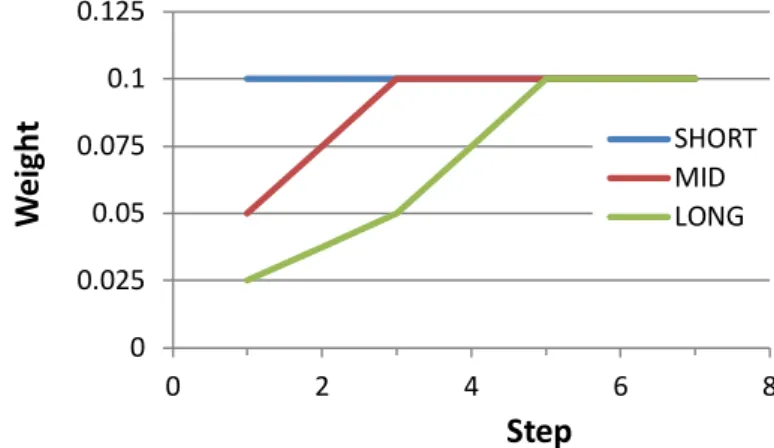
In iModeler the strength of influences develops differently according to the term, as shown in Figure 4. Note that specific delays can be entered directly in the properties box of an influence. Giving a delay greater than 5 means that the factor will not develop even at long-term.
Figure 4: evolution of delayed influences of strength 10 (10%) with each FCM iteration
Qualitative FCM has limitations that prevent us from fully specifying our perception of the Socio-Eco-System (SES), which can result in frustration from stakeholders (not seeing their viewpoint in the model) or misleading (assuming that their viewpoint is taken into account and reflected in the results). Over the process of modelling within EcoAdapt, we were confronted with the following cases.
Allocation
Allocation, e.g. allocating from a fixed water volume, a % of water to user A and to user B is tricky to implement in qualitative FCM. Let’s look at what happens if we allocate 70% water to Tabaco and 30% to cattle. With Menu>View>direct impact the FCM looks like:
0 0.025 0.05 0.075 0.1 0.125 0 2 4 6 8
We
ig
ht
Step
SHORT MID LONGAnd the insight matrix (see next section for more details on the insight matrix) for “Agua zona de riego” looks like:
Then we add an influence of -100% between %Tabaco and %Ganado (if %Tabaco increases, %Ganado decreases of the same value), the FCM looks like:
The effect of %Tabaco is the greatest (110) and %Ganado the smallest (-10), and one can see that the loop puts these factors away from the x-axis (see section below for more details on the insight matrix). Showing the indirect impacts (Menu>View>indirect impacts) the FCM looks like:
The sum of indirect impact from the two arrows coming out of %Tabaco and of %Ganado are 110 and -10 respectively (same as x-axis of the insight matrix). How do we interpret this result? Let us cluster the %Ganado and %Tabaco under category Water Allocation, which gives:
We find, as expected, that Water Allocation is the strongest factor affecting Agua zona de riego. Therefore the allocation factors have to be clustered in order to have meaningful results.
Factor values
Be careful that qualitative FCM is not to be interpreted as a classic FCM. In a classic FCM the effect of a factor A on Factor B is the value of that factor times the influence it has on factor B. In that case,
the value of a factor A that receives a lot of negative influences may become negative after a few iterations (except if we use squashing functions that limit its value to 0), then its influence may become negative! It is not the case for qualitative FCM (iModeler style), where influences are independent of factor values and factors have a constant, virtual value of 1.
Uncertainty
Uncertain (i.e. as random or stochastic factors values or influences) cannot be implemented in a qualitative FCM (but it can in a quantitative one, see section 2.6).
Reversibility
Reversibility (irreversibility is inherent to causal models) can be partly taken into account by understanding tradeoffs. For example, if a farmer invests in perennial crops like coffee, it has less money to invest in sugarcane. Therefore you can put negative influence between coffee and sugarcane, or between coffee and farmer investment.
Periodic fluctuations (e.g. seasonality), stochastic factors, discrete events
Classic FCM is not appropriate to take into account factors that are random, appear then disappear, or have fluctuations in amplitude. In the case two seasons must be considered, one can have a FCM for dry season and a FCM for wet season, or a factor for the dry season and a factor for a wet season.
Constraints
Constraints such as thresholds and limiting values are difficult to implement in qualitative FCM. For example, similar to the Allocation problem above, when trying to represent a change in land use for a given territory, e.g. pasture area increases at the expense of forest area (%forest+%pasture=100), i.e. more forest area leads (immediately) to less pasture area and vice-versa, since the total area is constant. One way to take this into account is to put a negative influence of 100% between forest area and pasture area (and vice versa) and cluster these factors into e.g. Land Cover category (see Allocation).
6.2. Examine model and results (iModeler)
Qualitative, explorative models easily grow to hundreds and thousands of factors. iModeler implements features similar to how our brain forms chains of arguments and thoughts. We can change perspectives of the model and navigate back and forth between them, show or hide levels of
compressed view of your models (Menu>Preferences), which is extremely useful when single factors are influenced by a bunch of factors which clutter the screen. Many options are accessible via the Menu.
Perspectives and levels of details
To put the current central factor back to the middle of the screen you can click/ tap on this icon on the upper left of the screen. You will notice that clicking/tapping on it the model shows just one level of connections of the central factor. Another click shows two levels and a third click shows all connections:
Clicking on this icon (which appears when one click on a given factor) puts it at the center of the screen and reorganize factors (showing hidden levels). This is very useful as many models become very huge and difficult to read: you can literally tell a story around a factor that your viewers can follow far better than it would be possible if you had shown all the connections at once.
On the upper right of the screen you may navigate back and forth through the various perspectives you have taken during exploration of the model.
On the upper right of the screen, there is a “Search” box to get to a factor. >> displays login info and account settings.
These buttons at the bottom right of the screen allow changing the zoom and fisheye intensity of the view.
You can move the positions of factors temporarily, e.g. for presentation in the iModeler Presenter (see below) or simply to have a better look at connections that are overlapping. The positions will reset as soon as you change the perspective again. You can save these positions via the properties of the current central factor (toggle between user-defined positions or automatic positioning). You can also use colors, shapes, and description texts (see below), through the properties dialogue of connections and factors. It is very useful to allocate the same colors to factors you want later to compare within the insight-matrix (see below). You may even use different shades of the same color to indicate an additional dimension of information, e.g. the current state of a factor within a project or the likelihood of an incident. Then the insight-matrix shows that a factor is very import, and the intensity of the color you have chosen indicates whether this factor is likely or still to be done.
Categories
Through the factor properties box (above) you can define any category you want and assign (even multiple of them) to the factors, to represent higher level concepts or group various concepts from different stakeholders world view. The categories then can be edited, the color and the shape be changed so any not otherwise customized factors will get that color. Having assigned categories we can choose the Menu>View>Filter/Cluster and select which factors you do not want to see in the model and hence filter, or which factors should be presented summed up as a cluster. We can even look at the sum of all the clusters including factor’s impacts in the insight matrix. The status bar at the bottom of the window indicates whether a cluster or a filter is being used, and when it is the connections between clustered factors appear as dotted arrows. Categories are useful to limit the
Connections
Alternatively you can look for a list of connections between two factors via Menu>Show connections. In many cases we draw redundant connections that may lead to clouded results, and this can help identifying them. It is also possible to add connections labels and descriptions through the
connection properties box.
Viewing Indirect and Direct impacts (only meaningful in qualitative modelling)
With Menu>View>Direct impacts, the strength of influences is displayed on the FCM. With
Menu>View>Indirect impacts what is displayed is the effect of each factor on the central factor. One can see that the farther a factor is from the central factor, the lowest the impact.
Note that the sum of all indirect impacts on a factor correspond to the x-axis of the insight matrix.
Viewing Loops (only meaningful in qualitative modelling)
Loops are displayed with Menu>View>Loops. Loops can be either balancing or reinforcing. Reinforcing feedback loops lead to a somehow arithmetic growth of factor’s influence, while balancing feedback loops dampen the system. The iModeler shows only the shortest first 1.000 loops (in general only shorter loops should have a significant Impact). If you want to see in what loops a certain factor is involved you can use the Search box to filter the set of found loops. The loops are then shown in your model with red colored connections for the reinforcing feedback loops, and blue connections for the balancing ones. Connections that are part balancing and reinforcing feedback loops have both colors. For some loops you need to change the perspectives of your view to see them completely.
Insight Matrix (only meaningful in qualitative modelling)
The Insight Matrix is an extremely important feature unique to iModeler that allow identifying the drivers that have the strongest (or weakest) effect on a given factor for the short, middle and long term. The Insight Matrix is displayed by clicking on “Insight Matrix” button at the bottom of the factor’s properties box.
The insight matrix computes the sum of assumptions and the chain of impacts on a given factor and displays it in a two-dimensional graph. On the horizontal axis what impact the other factors have on the selected factor. Thus we see what measures promise to comparable effective and what not, or what risks might become more crucial than others. On the vertical axis how this impact might change medium and long term due to delays and feedback loops (i.e. if there are no loops in the system and if delayed influences have fully developed at a given time, then all factors align on the horizontal axis for that time). The farthest from the center of the graph, the most pronounced the direct effect (x-axis) or effect of loops (y-(x-axis).
• Factors that are in the Blue area are those that decrease the value of the factor of interest, an effect that will decrease in the future.
• Factors that are in the Green area are those that increase the value of the factor of interest, an effect that will increase in the future.
• Factors that are in the Red area are those that decrease the value of the factor of interest, an effect that will increase in the future.
• Factors that are in the Yellow area are those that increase the value of the factor of interest,
an effect that will decrease in the future.
In general terms:
• Delays on positive influences show up in the Blue and Green areas, while delays on negative influences show up in the Red and Yellow areas.
• Balancing loops show up in the Blue and Yellow areas, while Reinforcing loops show up in the Red and Green areas.
Which means that for a model without delays or loops, all factors align on the x-axis.
Technically, the insight matrix computes (with proprietary algorithms) the short; mid and long term impact of the propagation of sudden increase of the value of each factor (from 0 to 1) on the factor of interest. For example is factor A has a weak influence (10 impact points) on central factor B, factor A will appear in the insight matrix at x-coordinate = 10, in other words a change of value of factor A from 0 to 1 will create an impulse of strength 0.1 (10 impact points) onto factor B.
You may give factors that represent measures, goals, risks, resources etc. the same color so it
becomes easier to compare them in the Insight Matrix. You can select a subset of factors to display in the insight matrix. You can also click on the factors in the list on the right side to see their values in the matrix, or directly on the points within the matrix to see on the list what factor it is. If there are several superimposed factors you can highlight them (dark blue) on the right side by clicking on the point in the graph; you may also chose if you want to display x/y coordinates as point labels. Filters allow choosing whether you want so see or not the factors with the chosen categories. Data from the insight matrix can be exported by clicking on “Export data” at the bottom of the screen (note that it also exports longer than long-term effects).
You can also zoom areas of the matrix and move the zoomed area by dragging. The insight-matrix cannot show you the value of a factor or when something occurs, but it allows you to identify large risks as well as crucial leverage points. This lets you to gain insight from those fuzzy, rough
assumptions better than any sophisticated formula could have.
Let us take the simple example developed above (remember that there are no loops and that is a long-term delay for the influence of Pollution to Water treatment plants):
The insight matrix for factor Water quality is as follows. In the short term, Pollution (x = -24.3; y = 0.7) has the strongest negative impact, an impact that will decrease in the future (due to the delay – there are no feedback loops involving Pollution). Water treatment plants (x = 17; y = 0) has the strongest positive impact that stays the same in the future (no delays nor loops).
In the mid-term, as expected, Pollution (x = -24.3+0.7 = -23.6, y = 1.4) has slightly less impact on Water quality than in the short term (this impact will be even more reduced in the long term – y = 1.4 instead of 0.7) while Water treatment plants has the same impact as before.
In the long term, all factors align on the x-axis, indicating that there is no more effect of the delay between Pollution and Water treatment plants.
Now this could look counter-intuitive. How can we explain that the effect of Water treatment plants on Water quality does not change with time, when it is likely that the number of water treatment plants may change over the course of a simulation? Remember that the direct effect of this factor on Water quality does not change over time. The change of the number of Water treatment plants is due to Pollution monitoring, so it is this latter factor that matters. Note that one can generate an impact matrix for these factors to gain insight on what can be done about it.
Based on these insight matrices one can decide: to improve the throughput of Water treatment plants (e;.g. impact on Water quality could be strong i.e. 25), decrease the delay to deliver new water treatment plants or increase pollution monitoring frequency. Pollution being a consequence of activities by Residents and Tourists, and Tourists contributing the most, we can focus on improving tourism infrastructures or implement stronger policy for responsible tourism (these can be new factors to include in the model).
Note that in many classic FCM simulations of complex systems, the value of factors shows transient behavior (essentially model artifacts) then stabilize after a few iterations (Kok, 2009). Therefore if the FCM is meant to represent the actual, steady state situation, it is advisable to examine long-term behavior (e.g. in the impact matrix) when all influences have reached their full strength and all factors values are more or less constant, then short term which change rapidly with time.
The Presenter
Larger models offer a large number of insights from different perspectives onto the model, from different insight matrices. To show them live in front of an audience can be a challenge as you have to keep in mind what to show and have the participants wait until the calculations are computed. This can be speeded up by using the iModeler Presenter (Menu>Presenter). There you can collect views from your model and build a presentation of them. You can change the order of the pictures via a button to move one picture one position up. Also you can show your presentation in full screen view.
Speech input
If using Google Chrome you can speed up your modeling using Speech input. In the Menu>Preferences check “Speech Input”, then you can directly click or tap onto the
microphone symbols of the buttons for the incoming our outgoing buttons of a factor to spell the name of other connected factors. This feature is not very useful in Spanish but it is good to know it exists!
Shortcuts
iModeler offers several contest-sensitive shortcuts to speed-up model development and visualization:
6.3. Documenting and versioning
Save model versions
Models are automatically saved in the cloud, so only one version is kept. Maintaining various version is a bit tricky. Via Menu>Export model> you can backup your model, which will save it as a text file with extension “.imm”. Then you can edit the text file to change the model name (e.g. “La cienaga v1.0”), which you can load again via Menu>Import. This allows you to keep various versions of the model in the cloud.
Open models
Using the cloud you have two ways to search for models: You can choose to include all models from the cloud (“All”) and you can choose to look for models with factors that match your search term (“More”). Alternatively you can sort the table of models by clicking on the headers.
Documenting models
The time units and horizon of the model can be specified via Menu>Properties>. This has an effect on calculations only in Quantitative FCM.
This way of documenting is useful but limited, e.g. it is impossible to have an overall picture or good traceability. We strongly suggest you keep an excel file (this would allow e.g. calculation of relative weights) that documents units, stocks, delays, and evidence to support your choice of weight (ranking, opinions, documents, calculations, data), e.g.:
Factor Description factor (units)Quantity of Evidence to support (opinion) Links to docs Links to data Estimation
Calidad del agua concentration of water pollutants 10ppm coliforms Report from Intendencia
Weighting matrix
Influencing Factor Weight [%] Description of factor factor (units)Quantity of Delay Evidence to support (opinion) Links to docs Links to data Estimation
Turistas -25 pollution from tourists per year 5T/yr 0 estimate of number of tourists from camping managers (12/2012)
Bosque 1 Decontamination from Forest area per year 1T/yr 0 GIS
Campos -1 pollution from Agricultural Fields area per year 10 (ha) 0 GIS
Deporte aquaticos -5 pollution from recreation boats per year 100 (yr-1) 0 estimate from camping managers (12/2012)
Ganado -5 pollution by cows near water per year 50 0 visual estimate
Habitantes -5 pollution by houses near water per year 15 0 visual counting
Pescadores -5 pollution by fishermen per year 10 0 estimate from camping managers (12/2012)
Usarios de vehiculos -5 number of cars in roads near water per year 50 0 estimate from camping managers (12/2012)
Volumen 48 yearly average of volume of water in dam 0 equal to sum of all pollution
7. Quantitative modeling
With Quantitative Modeling we are looking at time series. Data and mathematical functions will define the behavior of factors in our model, as well as scenarios. Qualitative modeling shows what is important, and quantitative modeling shows how something might develop.
In this section we briefly explain how to model quantitatively with iModeler, and how to implement a classic FCM (without squashing functions).
In iModeler quantitative modelling is done in the same interface than iModeler qualitative mode (systems dynamics mode). This can be confusing, because many functions are meaningful only in either mode, and some are interdependent. For example, the insight matrix is computed based on qualitative weights, not on the quantitative ones, while time series are meaningful only in
quantitative mode. Qualitative delays are used for quantitative mode, but as soon as delay() is used in a formula, “f(x) will appear in the properties box, instead of the qualitative delays.
When one clicks on “Formula” in a factors properties box, the formula editor appears (to go back to qualitative mode click on “Relation”). Then one can click on one of the mathematical functions available (here “relative quantification”) which gather information from the qualitative weights. The list of contributing factors appears on the top, and are used in [] in the formulas.
Classic FCM with iModeler
It is very easy to implement a classic FCM (without squashing functions) with iModeler, provided we understand its mechanics. As an example, we will program the FCM from Kok (2009) given in figure 3. In iModeler the FCM looks like this (note the absence of self-reinforcing loops):
The formulas are the following, and that one has to specify an initial value. It also uses valuebefore() for self-reinforcing loops.
C1: if(time()==1;1;[C2]*(-0.1)+valuebefore(1)) C2: if(time()==1;0;[C1]+0.5*[C3])
C3: if(time()==1;1;valuebefore(1)-0.5*[C2])
Clicking on “Cockpit”, one can then perform a simulation and obtain the curves of Kok (2009)
showing the evolution of factor values (in Menu>Model properties> we have specified a time horizon of 31 steps). Note that iModeler will ask to add delays for meaningful simulations (this because it considers factors as stocks while classic FCM does not).. just say no in order to have complete control on the delays.
We can go further than Kok by implementing uncertainty on one factor. Let suppose the initial value of C2 can be between -0.5 and 0.5. This is done by modifying the C2: formula as follows:
if(time()==1;range(0;1;0.1)-0.5;[C1]+0.5*[C3])
Accept the fact that 10 simulations will be done, then click on “Full Screen” the on the “MC/OR” button to show individual time series for each value of the initial parameter. One can see that the long-term values of C2 are insensitive to this variation in the initial values of C2.
To test new alternatives from a steady-state situation, one can change the initial values of factors by their long-term values. But if there are lots of transient and long term values are very different than initial values, then you may have a second look at your initial conditions and model structure (balancing loops may be missing).
Steps to define a quantitative model in iModeler. 1) Design your model as in qualitative mode
2) Define the time unit for your simulation and the time period you want to run scenarios of. You can do this in the Menu>Mode Properties
3) Define factor values. There are three ways to do so:
a. Via an input factor, i.e. a factor that is not defined by other factors from the model and hence needs to get its values over time directly, either by a constant you define in the formula field or by an input series that you can drag directly into the diagram, insert into the table or import from external data sources
b. Via a formula to describe the effect that incoming factors have onto the selected factor, i.e. how the values of the other factors from each time step result in the value of the current factor at the same time step. To see whether your model is completely quantified and the formulas are correct you can choose the Menu>View>Quantitative validation.
c. You can define a factor’s values as a related to the values of another factor by a graphical function or a table with relation values.
4) Perform The simulation: choose whether you want to look at a table or a graph, add up to 4 factors that you want to compare with a selected factor and then choose either to simulation
the whole scenario (>) or just step after step (>|).For more details click on “Full screen” and there you can even add parameters that you can use to alter the scenario.
Scenarios
In the full screen mode of the cockpit of each factor you can click on “Scenario” to save the current set of parameters of the model. This way you can quickly compare different scenarios. Note that just the parameters are saved - not changes of the model structure.
Uncertainty and Monte-Carlo-Simulation
If you use random(), likelihood(), gaussrandom() or other random functions to represent uncertainty within your model, iModeler asks how often you would like to simulate your model to come up with a range of possible outcomes. The result can be seen in the full screen modus of any factor’s cockpit. There you can click on “MC/OR” to see a spaghetti diagram. With the help of the zoom function you can click on any curve to choose the scenario that led to its values. When you have chosen a scenario all other factors show its values. Another click on “MC/OR” switches to a histogram where see the likelihood of certain outcomes at a certain point of time (click on one bar to see the value). The great challenge of this analysis is how we can translate these graphs (e.g. for evaluation of alternatives) into something that speaks to non modelers.
Sensitivity analysis via the Range() Function
The range() function has two purposes: 1) to automatically run a set of scenarios for a range of parameter values (sensitivity analysis). 2) to identify optimal parameter combinations in the sense of Operations Research optimizations. Just define a range for each parameter and the iModeler tries (brute force) all possible combinations. In the full screen modus then you can click on the curve that shows the scenario you want. You can then look for the parameters of this scenario, i.e. your optimal solution.
Note on calibration of classic FCM
Calibration is a critical step for any model (in qualitative mode we would rather use the term “validation”). The semi-quantitative nature of the factor values, however, limits the applicability of standard calibration methods used for quantitative models. One way to address these limitations is to make the underlying assumption that the system is in or near equilibrium. Therefore, the FCM long-term, stable factor values should compare to observed values, which is indicative of the quality of the model. Another way is to use existing information on changes of the value of specific factors. Sensitivity analysis is also useful to determine those factors that are important, those that may diverge or oscillate (which would require a more careful examination of the initial values, influences and feedback loops) and those for which the system is insensitive (robustness of factors – this is
useful for assessing the robustness of alternatives in our S&S process). Note that deviation from initial conditions reflects the fuzziness of our understanding of the system!
An entry-level, practical description of the logics and evaluations behind classic FCM (and their limitations) is provided as tutorials at http://www.ochoadeaspuru.com/fuzcogmap/tutorial.php. See for example how they failed to simulate increased demand of computers in a simple offer and
demand case, while it succeeded to provide reasonable predictions of how the weather affects traffic congestion, patrol frequency, risk aversion and driving speed
iModeler mathematical functions to use in quantitative modelling
The following table lists all the mathematical functions available, their description, parameters, and examples.
Stock Description: Stock factors are known from system dynamics. With a delay of one time step they sum up their values adding or subtracting the values of flow factors that point to them.
Example:
valuebefore(0) +delay0(1; [Factor1])+delay0(1; [Factor2])-delay0(1; [Factor3])
Relative_quantification Description: Puts the weight of the qualitative connection as a factor in front of the factors in the formula Example:
0.17*[Factor1]+0.23*[Factor2]-0.45*[Factor3] Multiplicative Description: All incoming factors are muliplied
Example:
[Factor1]*[Factor2]*(-[Factor3])
Additive Description: All incoming factors are added Example:
[Factor1]+[Factor2]-[Factor3]
Non_Negative Description: Avoids a negative result of the formula. If it is negative, it will be set to 0 Example:
if(([Factor1]) >= 0;([Factor1]);0)
abs Description: Computes the absolute value Parameter: value
Factor, value or formula Example:
-3.2 returns 3.2
acc Description: Sums the values of a factor or a number Parameter: value
Factor oder number that is summed up Example:
acc([Factor1])
and Description: Extension of if function, allows to form logical combinations Parameter: if Condition 1 Parameter: and Condition 2 Parameter: then then case Parameter: else else case Example: if(2==2 and 3==3; 4; 5)
arctan Description: Returns the arc tangent of an angle Parameter: arg
The value whose arc tangent is to be returned Example:
arctan([Factor1])
average Description: computes the moving average of a value for a chosen interval Parameter: past
time stamp for average Parameter: input a factor Example:
average(1; [Factor1])
condense Description: computes sums of a factor for the chosen time unit, possible time units are years(), halfyears(), quarters(), months(), weeks(), days(), hours(), minutes(), seconds().
Parameter: timeunit time unit Parameter: formula a formula or a factor Example: condense(months(); [Factor1])
cos Description: Cosine function
Parameter: arg Angel in radians Example: cos([Factor1])
date Description: allows to compare the current time step with a date Parameter: format
a date with format dd.mm.yyyy Example:
if(time()==date(23.10.2012);1;0)
day Description: allows to extract the day of the current time step Example:
if(day()==15;0;1)
decade Description: allows to extract the decade of the current time step Example:
if(decade()==8;0;1)
delay0 Description: Takes the value from a factor the number of time steps before Parameter: delay A delay value Parameter: factor A factor Example: delay0(5; [Factor1])
exp Description: Exponential function Parameter: arg
the argument Example: exp(1) => 2.71
gaussrandom Description: random function combined in one factor with the relation with the gauss-values Parameter: mean Mean value Parameter: sigma Standard deviation Example: gaussrandom(0;2)
halfyear Description: allows to extract the half year value of the current time step Example:
if(halfyear()==2;0;1)
hour Description: allows to extract the hour of the day of the current time step Example:
if(hour()==23;0;1)
if Description: If function. If functions can be combined Parameter: if Conditional Parameter: then then case Parameter: else else case Example:
if(2==4; 3;8) => 8, if ([Factor0] < 10; if([Factor1] <= [Factor2];[Factor3];[Factor4]; 1) int Description: Rounds down a value to an integer
Parameter: value Any value or factor Example: int(3.75) => 3
likelihood Description: activates the monte-carlo simulation and returns 1 with the defined likelihood, else 0 Parameter: value
A value between 0 and 100 Example:
Parameter: arg Any value Example: log10([Factor1])
logn Description: the natural logarithm Parameter: arg
Any value Example: logn([Factor1])
max Description: Computes the maximum of a list of parameters Example:
max(30; 10; 50; 40) => 40, max([Factor1];[Factor2];[Factor3]) mean Description: computes the arithmetic mean of its arguments
Example: mean(3; 3; 6) => 4
min Description: Computes the minimum of a list of parameters Example:
max(30; 10; 50; 40) => 10
minute Description: allows to extract the minute of the current time step Example:
if(minute()==53;0;1)
month Description: allows to extract the month of the current time step Example:
if(month()==9;0;1)
not Description: not-addition to the if-function, allows to form combinations Parameter: not
not condition Example:
if(not(1==2);3;4)=>3
or Description: or-addition to the if-function, allows to form combinations Parameter: if Condition 1 Parameter: or Condition 2 Parameter: then Then case Parameter: else Else case Example: if(1==1 or 2==3; 4; 5) => 4
pi Description: The value of pi, approximately 3.14159265. Example:
pi()
pow Description: Power term
Example: pow(2; 3) => 8
pulse Description: returns 1 from the defined start time for the defined number of time steps Parameter: start
the start time Parameter: length the duration of the pulse Example:
pulse(time() == date(5.12.2010) or(time() == date(12.12.2010)); 4) quarter Description: allows to extract the quarter of the current time step
Example: if(quarter()==2;0;1)
random Description: Activates the monte-carlo simulation and returns a random number between 0 and 1. Example:
random()
range Description: Within a simulation multiple simulation runs for this factor are performed. For models with more than one range function all range combinations are simulated. So optimal factor combinations can be identified. Parameter: from Start value Parameter: to End value Parameter: step Step size Example: range(10;20;2)