Computing Delay-Constrained Least-Cost Paths for Segment Routing is Easier Than You Think

HAL Id: hal-02993545

https://hal.archives-ouvertes.fr/hal-02993545

Submitted on 6 Nov 2020

HAL is a multi-disciplinary open access

archive for the deposit and dissemination of

sci-entific research documents, whether they are

pub-lished or not. The documents may come from

teaching and research institutions in France or

abroad, or from public or private research centers.

L’archive ouverte pluridisciplinaire HAL, est

destinée au dépôt et à la diffusion de documents

scientifiques de niveau recherche, publiés ou non,

émanant des établissements d’enseignement et de

recherche français ou étrangers, des laboratoires

publics ou privés.

Computing Delay-Constrained Least-Cost Paths for

Segment Routing is Easier Than You Think

Jean-Romain Luttringer, Thomas Alfroy, Pascal Mérindol, Quentin Bramas,

François Clad, Cristel Pelsser

To cite this version:

Jean-Romain Luttringer, Thomas Alfroy, Pascal Mérindol, Quentin Bramas, François Clad, et al..

Computing Delay-Constrained Least-Cost Paths for Segment Routing is Easier Than You Think.

IEEE International Symposium on Network Computing and Applications, Nov 2020, On-Line, France.

�hal-02993545�

Segment Routing is Easier Than You Think

Jean-Romain Luttringer

, Thomas Alfroy

, Pascal M´erindol

, Quentin Bramas

, Franc¸ois Clad

, Cristel Pelsser

Abstract—With the growth of demands for quasi-instantaneous communication services such as real-time video streaming, cloud gaming, and industry 4.0 applications, multi-constraint Traffic Engineering (TE) becomes increasingly important. While legacy TE management planes have proven laborious to deploy, Segment Routing (SR) drastically eases the deployment of TE paths and thus became the most appropriate technology for many operators. The flexibility of SR sparked demands in ways to compute more elaborate paths. In particular, there exists a clear need in computing and deploying Delay-Constrained Least-Cost paths (DCLC) for real-time applications requiring both low delay and high bandwidth routes. However, most current DCLC solutions are heuristics not specifically tailored for SR.

In this work, we leverage both inherent limitations in the accuracy of delay measurements and an operational constraint added by SR. We include these characteristics in the design of

BEST2COP, an exact but efficient ECMP-aware algorithm that natively solves DCLC in SR domains. Through an extensive performance evaluation, we first show that BEST2COP scales well even in large random networks. In real networks having up to thousands of destinations, our algorithm returns all DCLC solutions encoded as SR paths in way less than a second.

I. INTRODUCTION

The fundamental challenge addressed by a routing scheme is about deploying best paths. Internet Service Providers (ISPs) usually compute such paths according to a single additive metric, the IGP cost, which models the available resources of the network. Generally, the IGP distance takes into account the bandwidth of each link and is further tuned to reflect the specific needs of the ISP. While it is sufficient for best-effort traffic, real-time flows have strong additional requirements in terms of delay. Our discussions with network equipment vendors indeed revealed a strong demand for ways to compute paths providing the maximal possible amount of bandwidth (to ensure a high flow quality) among the ones verifying a constraint on the end-to-end delay (the maximal latency for interactive real-time flows). In practice, the considered delay metric is the measured propagation delay. However, the bandwidth is not considered per se. Actually, the second considered metric is the IGP cost. Indeed, since the latter is representative of the bandwidth as well as the ISP’s specific needs, finding paths minimizing the IGP cost among the paths respecting the delay constraint allows the user to experience a low propagation delay and high bandwidth route while preserving the ISP resources.

Computing such paths requires to solve the problem known as DCLC (Delay Constrained Least Cost). This problem has attracted a lot of attention from the research community [1].

Despite only considering two (additive) metrics, DCLC is known to be NP-hard [2]. Indeed, two dimensions are enough to turn the total ordering existing with a single metric into a partial one, as any path better on at least one metric compared to currently known paths may be part of the solution and thus has to be explored. These paths are referred to as non-dominated paths and make up the Pareto front of the solution. To solve DCLC exactly, the whole Pareto front (2-dimensional because the problem is limited to 2 metrics) must be explored. Since the latter may grow exponentially, this family of problems is considered intractable.

Several approximations schemes exist to solve DCLC. How-ever, these latter have never been deployed by operators as they do not provide sufficient guarantees in term of performance and rely on a technology that does not scale well. In this work, we show that DCLC can be solved exactly and efficiently without neglecting the practical deployment of constrained TE routes. As long as two reasonable practical assumptions are verified, it is possible to build an efficient algorithm.

Our first assumption concerns the nature of the metrics. Due to the apparent intractable nature of DCLC, most current solutions rely on heuristics, which are complex to deploy and do not offer strong guarantees in all cases. However, although DCLC is computationally expensive, its complexity is often misinterpreted. Exponential cases are unlikely to occur in prac-tice [3] thanks to the structures of ISP networks and the fact that their metrics lead to a limited number of distinguishable distances. As soon as there exists few distinct values in the Pareto front, it is possible to bring strong guarantees without relying on heuristics. Our first assumption then is that either the IGP cost or the delay metric is bounded and discrete. While this requirement may seem strong, we argue that these metrics already meet it, the delay in particular. Indeed, IGP distances only provide relative bounds on the Pareto front size as they ultimately depend on the ISP configurations (although limited by the routing protocol itself). Conversely, the bounds provided by the delay are absolute (as they do not depend on any configurations) and often even stricter than the IGP routing limits, due to both physical limitations and the nature of delay-constrained flows. A real-time interactive flow must meet strict guarantees regarding its delay (at least < 100ms, usually closer to 10 or even 2ms). In addition, even though the precision in memory of the measurements can be high, i.e., nanosecond, no delay measurement technique can claim to be that accurate in worst-case scenarios. ISPs are aware that measured delays are an estimation, not a guarantee. These

©IEEE, 2020. This is the author’s version of an article that has been published in the NCA conference. Changes were made to this version by the publisher prior to publication.

delays (usually measured with OWAMP [4]/TWAMP [5]) have a limited trueness (as defined in ISO 5725-1 [6]) or accuracy, even with efficient hardware PTP time stamping systems or accurate two-way delay estimators. Due to both its inherent variation depending on physical properties, clock synchronization or inconstant packet processing delays [7], [8], we argue that truly distinguishing the delay of a path at the granularity of the micro-second is difficult if not impossible nowadays. Even the finest delay estimation is bounded and discrete by essence, allowing us to predict the size of the Pareto front and control the complexity of our algorithm.

Our second assumption concerns the technology at play. Current solutions do not usually consider the deployment of the computed paths. Consequently, they rely on RSVP-TE which does not impose any additional constraints on the paths to deploy. However, they thus scale poorly as RSVP-TE suffers from well-known scalability issues since both the number of control-plane messages and of forwarding states scale with the quantity of TE paths [9]. We thus design our algorithm for a specific technology, Segment Routing [9] (SR). SR is the new state-of-the-art TE and fast-reroute technology now deployed in most ISPs. SR relies on a very lightweight control-plane as forwarding states are carried within the packets. More precisely, SR implements source-routing by translating forwarding paths into lists of segments (routing instructions). This list is then encoded within each packet and used by routers to forward said packet. However, the size of this list is limited, as only SEGMAX ≈ 10 segments may be imposed on each packet at line-rate with today’s best hardware. If handled naively, this new constraint can considerably increase the problem’s complexity, as it may seem necessary to explore a now three-dimensional Pareto front. We design our algorithm with SR in mind by exploring the solution space in a way that leverages the SEGMAX constraint. We are thus able to efficiently deploy segment lists that respect both a constraint on their sizes and their delay while minimizing the IGP distances.

In summary, we leverage the two aforementioned properties (the inaccuracy of delay measurements and the SEGMAX con-straint) to provide a straightforward, efficient algorithm suited for practical TE usage: BEST2COP (Best Exact Segment Track for 2-Constrained Optimal Paths). BEST2COP is, to the best of our knowledge, the first algorithm able to solve DCLC efficiently in any scenario for large SR domains, and thus the first deployable DCLC scheme ever. In short, it com-putes all the paths verifying two constraints (delay and number of segments) while optimizing the IGP distances. BEST2COP can provide DCLC solutions for large realistic networks in a time period acceptable for the routing convergence, i.e., way less than a second.

In Sec. II, we formally define the 2COP problem for solving DCLC in an SR domain. Sec. III sketches BEST2COP before we evaluate its performance in Sec. IV. We conclude the paper discussing the related work in Sec. V and summa-rizing our achievements and future works in Sec. VI.

II. 2COP,ORSOLVINGDCLCWITHIN ASR DOMAIN

In this section, we formally introduce and define all nota-tions and concepts used to design BEST2COP. More precisely, we detail the problem we aim to solve, the construct we use to encompass Segment Routing natively, and how it is used to our advantage along with the delay characteristics.

A. Problem Statement, or the Need for an SR Graph

We aim to solve an SR variant of the DCLC problem, considering the IGP cost, the propagation delay, and the number of segments. We refer to this problem as 2COP. For readability purposes, we denote:

● M0 the metric referring to the number of segments, with

the constraint c0= SEGMAX ;

● M1 the delay metric, with an arbitrary constraint c1; ● M2 the IGP metric being optimized.

We also rely on these generic notations to highlight that the problem remains the same for any couple of metrics. Besides, the problem keeps the same complexity even if M2 is also a

constrained metric.

Definition. 2-Constrained Optimal Paths (2COP): Given a source s, 2COP consists in finding, for all destinations, a segment list verifying two constraints, c0 and c1, on the

number of segments (M0) and the delay (M1) respectively,

while optimizing the IGP distance (M2). We denote this

problem 2COP(s, c0, c1). ∎

BEST2COP solves 2COP by looking for all feasible dis-tances (i.e., satisfying c0 and c1) optimizing M2. Note that

2COP is distinct from DCLC because of c0. For example, let

us refer to Fig. 1 and consider DCLC for c1 = 7 from node

s to p. The solution is the path(s1, n)−(n1, o)−(o, p) having

an IGP cost of 4 and a delay of 6.49. However, the latter is not a solution of 2COP(s, 2, 7) towards p. Indeed, we will see that this path translates to three segments and violates c0= 2.

SR implements source routing by pre-pending packets with a stack of segments. Segments can be seen as a list of checkpoints the packet has to go through sequentially, be it a node or a specific interface. SR mainly uses two types of segments: node segments and adjacency segments. A node segment specifies a node as a checkpoint. A node segment representing a destination v is interpreted by a router as forward the packet to v (through the best IGP path(s)). Since SR enables ECMP by design, flows are load-balanced among best paths to v. On the contrary, an adjacency segment indicates that the router has to forward the packet through a specific local interface.

Thus, to encompass SR natively while solving DCLC, we rely on a structure for which the IGP costs, delays, and the number (and type) of segments used to build the segment lists are direct and natural properties. We call this structure an SR graph. An SR graph represents the segments as edges, whose weights are the (M1 ; M2) distances of the underlying path or

adjacency encoded by the segment.

Exploring paths on the SR graph is equivalent to exploring stacks of segments and the paths they encode. A path requiring

x segments is represented as a path of x edges in the SR graph (agnostically to its actual length in the raw graph). Thus, within an SR graph, one can simply check that x < c0 to

verify the constraint on M0. In an SR domain, the SR graph is

computed by default for any TE usages including fast-reroute. In our case, only some extra information needs to be added in order to correctly handle multiple metrics, which does not generate a significant overhead to the SR graph computation.

B. The SR Graph Construction

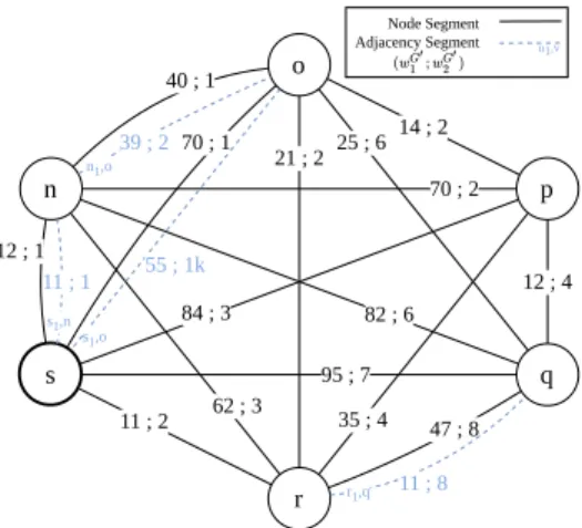
Throughout this section, we use Fig. 1 and 2 to illustrate the SR graph construction. While the former provides an arbitrary raw graph, the later gives its resulting SR counterpart. We start by describing the notations we use, in particular regarding multigraphs, as both the SR and raw graphs fall in this category.

Let G = (V, E) be the original graph, where V and E respectively refer to the set of vertices and edges. As G can have multiple parallel links between a pair of nodes (u, v), we use E(u, v) to denote all the direct links between nodes u and v. When necessary, we denote a specific link (ux, v),

x specifying the considered interface (a local number to u). Each link possesses two weights: its delay and its IGP cost. The delay and the IGP cost being additive metrics, the M1

and M2 distances(dG1 ; d G

2) of a path are simply the sum of

the weights of its edges.

From G, we create a transformed multigraph, the SR graph denoted G′= (V, E′). While the set of nodes in G′is the same as in G, the set of edges differs. Indeed, G′encodes segments as edges representing either adjacency segments (blue dashed edges encoding some adjacencies of G) or node segments, encoding sets of best ECMP paths. For instance, in Fig. 1, there exist three paths in G from n to r which have an optimal IGP-cost of 3: (n1, o)−(o, r) with distance (6.2; 3),

(n1, s)−(s, r) with distance (2.3; 3) and (n2, s)−(s, r) with

distance (2.4; 3). They are thus all represented by the unique link (n, r)G′ (in plain black in G′). When using a node segment specifying the destination r from n, the traffic is load balanced across the three paths.

Note first that we do not use 6.2 as the delay value in G′ but 62. Indeed, while the delay can be represented as a precise floating number, its actual accuracy is limited. We can safely round the M1-weights (delays) without losing relevant

discriminating information, reducing so the complexity of 2COP as we will detail in the following. Thus the path from n to r, relying on the best IGP distance (a node segment in G′), has distances (62; 3) = (40 + 22; 1 + 2), where 22 is the delay 2.15ms times 10 rounded up at the 0.05 accuracy grain. Second, we chose 62 in particular as the delay of the node segment because the only delay guarantee of a node segment is to not exceed the worst delay of all its ECMP paths.

In summary, a node segment encoding the whole set PG(u, v) of ECMP best paths between two nodes u and v is

represented by exactly one edge in E′(u, v). Its M2-weight,

w₂G′((u, v)), being the common M2-distance of PG(u, v),

s n o r p q 1.24 ; 1 1.15 ; 2 4 ; 1 1.11 ; 8 1.17 ; 4 1.37 ; 2 7 ; 1 7 ; 2 2.15 ; 2 5.5 ; 1k 2.16 ; 10k 3.9 ; 2 1.12 ; 1 3.65 ; 1000k s1 n₂ s₂s₁ n2 n1 n₁ s2 r1 r2

Figure 1: The raw network graph G= (V, E) is a multigraph, with weighted edges. The weight of the edges is represented as a couple (delay;IGP cost). While there sometimes only exist a single edges between two nodes, such as(s, r), we otherwise distinguish between parallel nodes such as(s1, n) and (s2, n).

its M1-weight, wG

′

1 ((u, v)), is defined as the maximum M1

-distance among all the paths in PG(u, v). Thus, links

repre-senting node segments in G′verify the following: w₁G′((u, v)) = max_P∈PG(u,v)dG₁(P )

w2G′((u, v)) = dG2(P ) for any P ∈ PG(u, v)

In addition to this unique node segment, E′(u, v) may contain adjacency segments (dashed blue edges in Fig. 2) to force the packet to go through a specific interface. An adjacency segment corresponds to an edge in the graph G and is represented by an edge(ux, v) in E′(u, v) whose M1

-weight, resp. M2-weight, is exactly the M1-weight, resp. M2

-weight, of the corresponding link in G. Note that if the node segment between two nodes has both a better delay and a better cost than any direct link between them, there is no point in using an adjacency segment. More generally speaking, an adjacency segment exists in G′ only if it is not dominated by other segments. Formally, an adjacency segment is represented by an edge (ux, v)G′ if it is not dominated by the node segment (u, v)G′, i.e., if dG₁((u, v)) > wG

′

1 ((ux, v)), or by

any other non-dominated adjacency segments numbered y, (uy, x), i.e., if w1G((uy, v)) > wG

′

1 ((ux, v)) or wG2((uy, v)) >

wG2′((ux, v)). For example, in Fig. 1, the best path from n to

o has a distance of(4; 1) and is translated to the node segment as a link with same values in Fig. 2. Since there exists another direct link between both nodes with a lower delay, (3.9; 2), we add an edge(n1, o) with distances (39 ; 2) to G′. One can

then force the corresponding adjacency segment to save delay. In practice, the SR graph G′ can be built for all sources and destinations thanks to any APSP algorithm to compute the weights of each node segment in G′. We consider this construction as a shared input for BEST2COP, as this trans-formation is inherent to SR and applies network-wide. Note that this computation is unlikely to be performed by the router itself, but rather by a Path Computation Element [10], which may be located within a controller. The overhead added to this construction by our specific transformation is negligible; it consists in the addition of the delay information, in particular to select non-dominated (adjacency) segments.

©IEEE, 2020. This is the author’s version of an article that has been published in the NCA conference. Changes were made to this version by the publisher prior to publication.

s n o r p q 40 ; 1 70 ; 2 82 ; 6 62 ; 3 12 ; 1 14 ; 2 25 ; 6 21 ; 2 70 ; 1 95 ; 7 12 ; 4 35 ; 4 84 ; 3 11 ; 2 _{47 ; 8} 55 ; 1k 11 ; 8 39 ; 2 11 ; 1 s1,n s1,o n1,o Node Segment Adjacency Segment _u1,v

r1,q

Figure 2: The SR graph G′(V, E′) encodes segments as edges. Plain black edges represent node segments, i.e., , sets of ECMP best path, while dashed blue edges represent link in the original graph G, making G′ a full-mesh at least. Adjacency segments, e.g., (s1, n), are only represented if they are not

dominated by other segments.

Thanks to this specific construct, we can now illustrate the sets of paths we want to retrieve when solving 2COP. We said in Sec. II-A that while path (s1, n)−(n1, o)−(o, p), having

a distance of (6.49 ; 4), solves DCLC for c2 = 7 and for

destination p, it does not solve 2COP(s, 2, 7). Indeed, we can now clearly see in G′ (Fig. 2) that to achieve this path, 3 segments are required: (s1, n)∣(n, o)∣(o, p), which makes it

non SR-feasible with a segment budget of 2. The solution to 2COP(s, 2, 7) is a list of 2 segments (i.e., a path of 2 edges in G′):(s, r)∣(r, p), encoding the path (s, r)−(r1, o)−(o, p) in

G. Note that this physical path has a distance of (4.6 ; 6). C. An SR Graph with True Measured Delays

In this section, we explain how the characteristics of real ISP networks are used to our advantage and translate in the construct we have detailed.

DCLC is pseudo-polynomial [11]. More precisely, it is polynomial in the smallest largest weight of the two metrics M1 and M2 (once translated to integers). As long as one

of the metrics possesses only a limited number of distinct values, the problem is tractable and can be solved efficiently, since the limited range of the metric restricts the number of non-dominated distances. The metric (and so, the number of distinct distances a path can have) can be bounded and its accuracy coarse by nature, or c1 can be small enough

to sufficiently reduce this number of values. Although our solution can be adapted to fit any metric, we argue that M1,

the propagation delay, is the best candidate and will, most of the time, have the lowest number of distinct values.

The delay is usually constrained through a strict bound (always lower than 100ms in practical cases). In addition, while the delay of a path is generally represented by a precise number in memory, the actual accuracy of the measured delay of an edge in G is far lower. Indeed, due to the inherent lack of accuracy of any delay measurements, discriminating

paths having less than a 0.1ms difference can be challenging if not impossible in the worst conditions. In that case, floating numbers representing the delays can be rounded to integer taking 0.1ms as unit. Since the delay is also bounded through its constraints, the number of distinct, discriminable delay values is likely to be very limited. This allows us to easily bound the number of possible non-dominated distances to c1×t, with t being the level of accuracy of M1 (the inverse of

the delay grain). For example, with c1= 10 (in ms) and a delay

grain of 0.01 ms, we have t= _0.011 = 100 and so only 1000 distinct (rounded) values to manipulate with BEST2COP.

In practice, this numerical value is controllable for solving 2COP even if c1is not a strict constraint. Indeed, let us recall

that we can also leverage the limited number of segments, c0

:= SEGMAX. We are limited to c0≈ 10 segments, i.e., paths

of 10 edges in the SR graph G′. Regardless of the constraint c1, we know that a feasible SR path will not exceed an M1

-distance of the maximum wG1′ weight on the SR graph times

c0. If we denote by S × t the maximum edge delay in G′

– once rounded to integer with an accuracy level of t – we know that a feasible SR path has a delay of at most 10×S ×t. In any cases, the number of possible distinct M1-weight of

SR-feasible paths in G′is bounded by Γ= min(c1, c0×S)×t.

For a rounded delay, it then becomes sufficient to store only the best M2-distance (indexed on its respective M1-distance),

leading to a Pareto front that can be stored in a static array of size Γ. In other words, there are at most Γ non-dominated pairs of distances to be stored and 2COP is polynomial in Γ. The complexity of 2COP is thus controllable. With a small enough delay constraint, the level of accuracy t of the delay can be increased and 2COP solutions can remain exact since 1/t becomes smaller than the inherent delay measurement error. Keeping constant the constraint-accuracy product makes the error margin constant relatively to c1. As an example,

maintaining Γ= 1000 with c1=100ms results in t= 10 and in

an error margin of 0.1ms. With c1=10ms, the accuracy level

t can be increased to 100, resulting in an error margin of 0.01ms. In all cases, the error margin is 0.1% relative to c1.

If c1 is a loose constraint, keeping Γ= 1000 results in weaker

approximations as t has to decrease, making the error margin become greater than the measurement inaccuracy. However, it allows the problem to remain tractable.

While the number of paths to manipulate in G′ is limited thanks to the aforementioned properties, it may be still con-siderable when V increases. Fortunately, we can once again leverage SEGMAX to cut down the exploration space. Since we are only interested in SR-feasible paths, we do not need to explore paths requiring more than c0segments. Using a variant

of the Bellman-Ford algorithm on the SR graph, this can be done easily as the path exploration naturally iterates over the number of segments, thanks to both the algorithm’s design and the SR graph representing segments as edges. BEST2COP visits G′ paths of i segments at its ith iteration, allowing us to stop after very few iterations at worst (all paths discovered afterwards exceed c0).

III. THEBEST2COP ALGORITHM

In this section we describe BEST2COP, our algorithm effi-ciently solving 2COP by leveraging properties formalized in the previous section. We propose here a high-level description, but the interested reader can find its implementation online1. While the implementation is designed for high performances, we omit here several details regarding its precise data struc-tures (even though these latter play an important role in BEST2COP’s overall efficiency). Like the SR graph compu-tation, BEST2COP can be run on a centralized controller but can also be directly launched by each router.

Simply put, at each iteration, BEST2COP starts by extend-ing the known paths for each node by one segment (i.e., one edge on the SR graph) in a Bellman-Ford fashion (a not-in-place version to be accurate); at the main difference that we consider here all non-dominated paths, i.e., the Pareto front. Second, newly found extended paths are filtered to reflect the new Pareto front. The remaining one will then be extended themselves, but not before the next iteration. Thanks to SEGMAX, these two steps only need to be performed≈ 10 times. Indeed, since we explore paths segment by segment, paths of i segments (i.e., i edges in the SR graph) are explored at iteration i. All paths not explored before the tenth iteration require more than SEGMAX segments and can be ignored.

The good performance of BEST2COP does not only result from a cut in the exploration space, but also from well-chosen data structures. Since the limited accuracy of the measurements bounds the number of non-dominated distances to Γ at each step, we can manipulate arrays of fixed size.

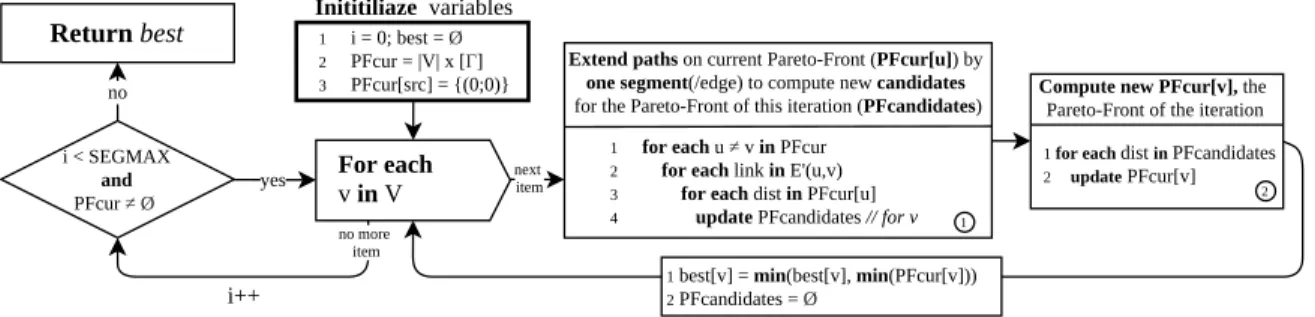
Fig. 3 sketches the main steps of BEST2COP. We focus on the PFcur structure for the sake of simplicity. The number of elements within PFcur is bounded by Γ. PFcur stores, for the current iteration and each vertex, the Pareto front of the distances indexed on their delay (M1). Since BEST2COP

explores paths segment by segment, PFcur will contain, at the ith iteration, all distances within the Pareto front encodable in exactly i segments. In particular, BEST2COP only needs to store in PFcur the best M2-distance for a given M1 index, as

we aim to find least-cost paths.

In the initialization, we set that the only known best distance is the distance to the source src itself,(0, 0) (i.e., PFcur[src][0] = 0). At iteration i (and as shown in box 1), for all predecessors u of each node v (i.e., potentially all u in V since G′is a full mesh), BEST2COP extends all the non-dominated distances to u (PFcur[u]) discovered at the previous iteration i− 1 by all weights in E′(u, v) (box 1, Line 2). By combining all distances to u discovered at iteration i− 1 with all weights of parallel links linking u to v in E′, we compute candidate distances of i segments towards v. Note that since M2-distance

towards v are indexed on M1, if a newly discovered M2

-distance is worse than the one currently sitting at the same M1-index, it means that the distance is dominated and that there is no point in keeping it (in box 1, it is basically the test performed in the update function of line 4). However, these

1_{https://github.com/talfroy/BEST2COP}

new distances to v may not be on the Pareto front as they can be dominated by other values newly discovered, stored in other indexes. We thus refer to them as PFcandidates. From the set of candidate paths, we still need to extract the new Pareto front of the current iteration (Box 2), which is stored in PFcur[v] and will in turn be extended at the next iteration. This is the purpose of the second update function that checks whether the candidate is actually non-dominated. For a given node, at the end of an iteration, the best known distances to it were correctly updated and will serve as a basis for the next iteration. We can then also safely record the current best path that minimizes the cost and respects by design the constraint c0 (using the array denoted best in the flow chart).

In reality, BEST2COP is far more versatile and able to optimize any of the three metrics (M0, M1 or M2) with

possibly constraints on all metrics. For example, referring back to Fig. 2, BEST2COP is able to return the solution to 2COP(s, 3, 70) towards p optimizing M0or M1((s, r)∣(r, p))

or optimizing M2 ((s1, n)∣(n1, o)∣(o, p)). In addition, with

only few adjustments on the returned structured, BEST2COP is able to return, upon a single run, all non-dominated distances respecting up to three constraints (c0, c1 and an additional

c2 in the most general case). Thus, if one decides to use a

stricter c1constraint, e.g., 2COP(s, 3, 65), the new constrained

path ((s1, n)∣(n2, o)∣(o, p)) can already be found within the

returned structure.

The time complexity of BEST2COP is showcased in the flowchart. For the ∣V ∣ possible neighbors of ∣V ∣ nodes, we extend up to Γ non-dominated distances by the L direct parallel links between them. This procedure is repeated up to SEGMAX times, leading to a time complexity of O(SEGMAX × ∣V ∣2_{× L × Γ).}

For the performance evaluations, we will consider that:

● SEGMAX = 10 as it matches current hardware capacity;

● L = 2: on average, in G′, one can expect that the total number of links in E′is lower than 2∣V ∣2. Indeed, adjacency segments are not likely to be numerous within transformed graphs, as they tend to be dominated;

● Γ = 1000: while controllable to reflect the expected product trueness-constraint on M1, we consider an

accu-racy level t of 10 (0.1ms accuaccu-racy) regarding a maximal constraint c1= 100ms.

IV. PERFORMANCEEVALUATION

This section evaluates the computing time performance of BEST2COP. We focus here solely on BEST2COP’s perfor-mances rather than relying on a comparison. As mentioned in Section I, most solutions rely on heuristics resulting in a poor exploration of the solution space in worst-cases. Conversely to these methods, BEST2COP provides controllable results and very good performance impervious to peculiar worst-cases. Furthermore, no existing schemes are specifically designed for SR. Upgrading them to handle SR raises several challenges, as minimal modifications would drastically increase their execution times. Such a fair comparison is left for future work.

©IEEE, 2020. This is the author’s version of an article that has been published in the NCA conference. Changes were made to this version by the publisher prior to publication.

Return best i < SEGMAX and PFcur ≠Ø no For each v in V no more item

Extend paths on current Pareto-Front (PFcur[u]) by one segment(/edge) to compute new candidates

for the Pareto-Front of this iteration (PFcandidates) Compute new PFcur[v], the Pareto-Front of the iteration

1 for each u ≠ v in PFcur

2 for each link in E'(u,v)

3 for each dist in PFcur[u]

4 update PFcandidates // for v

1 for each dist in PFcandidates

2 update PFcur[v] 1 2 yes i++ Inititiliaze variables 1 i = 0; best = Ø 2 PFcur = |V| x [Γ] 3 PFcur[src] = {(0;0)}

1 best[v] = min(best[v], min(PFcur[v]))

2 PFcandidates = Ø

next item

Figure 3: BEST2COP algorithm. BEST2COP works by exploring paths of increasing length on G′. Non-dominated paths are extending by one edge. The algorithm ends at the SEGMAXth_{iteration or when progress stops.}

First, it is worth to notice that without any graph-based assumptions except the ones mentioned above (i.e., just setting ∣V ∣ = Γ = 1000 and with an average of two parallel links per connection, L = 2), BEST2COP never takes more than one minute to explore its full iteration space. That is, when BEST2COP is forced to performs its maximum number of operations on any graph having these characteristics, solving 2COP cannot exceed one minute. This extreme upper bound is far from BEST2COP’s real performance, as its data structures were virtually filled up to push it to its limits. In practice, when considering concrete underlying networks, even random ones, BEST2COP can easily deal with average or worst-cases in less than half a second.

Conversely to the vast majority of existing evaluations related to TE routing algorithms, we focus on challenging scenarios implying large networks. Moreover, we do not rely on a strict delay constraint to simplify the problem. First, we only consider the largest one that is practically relevant to DCLC, c1< 100ms. Second, we do not ignore distances whose

pruning in the SR graph can reduce the exploration space, which stresses our solution as much as possible. Formally, our evaluations are designed such that BEST2COP returns, for all n∈ V , the whole 2COP (s, 10, 100) set.

Given the difficulty to find real or inferred graphs having two valuation functions, we leverage the characteristics of SR Graphs (namely, their fully-meshed structures) to generate numerous scenarios. We nevertheless conclude on evaluations performed on real ISPs with real IGP costs and delays. For all the evaluations, we rely on a 4,2 GHz Intel Core i7 CPU. While parallelizing BEST2COP through slight tweaking is possible, this additional evaluation is left for future work. We show here only the results of a purely sequential approach. A. SR Graph with Random Valuation

An SR Graph G′ is at least a full-mesh when the original graph G is connected. We use this convenient property to ease the generation of SR graphs for our evaluations.

We generate complete graphs of ∣V ∣ nodes having ∣E′∣ = 2∣V ∣2_{edges, creating so a double full-mesh graph. One}

system-atic additional link is enough to mimic unfavorable practical cases, as realistic topologies tend to possess a low average number of adjacency segments once converted. Regarding IGP weights, we chose them uniformly at random between

��� ��� ��� ��� ��� ��� ��� ��� ��� ���� �������������������� � ��� ��� ��� ��� ���� ��������� ����������� ��� ��� ����

Figure 4: BEST2COP worst-case when considering ran-domly weighted SR graphs with three spreading valuations. BEST2COP remains always under the second and scales decently regarding∣V ∣.

1 and 224 (the maximum possible IGP cost with current IGPs). Propagation delays are uniformly distributed at random between 1 and S = {100, 500, 1000}.

Since we set Γ at 1000, picking delay weights higher than 1000 (with a higher delay spreading) is too advantageous by design as many distances will exceed the constraint. We perform these tests for ∣V ∣ ranging from 100 to 1000 (with steps of 100). To account for the randomness of both valuation functions, we generate, for each ∣V ∣, 30 differently weighted distinct topologies, and run BEST2COP on ∣V ∣ × 0.1 nodes as sources. This evaluation is not advantageous as we do not benefit from any pattern generated by realistic networks. The resulting computing times are shown in Fig. 4.

This random weights evaluation exhibits the efficiency of BEST2COP: its execution time stays under one second in all of its runs. BEST2COP scales well enough with the dimension of the network which is the critical performance parameter (quadratic in ∣V ∣). It is also worth noticing that a spreading value of 500 leads to the worst time results (label S = 500), while a value of 1000 or only 100 leads to a slightly better or a very notable decrease in execution time respectively.

The M2distance spreading has indeed a great impact on the

of the Pareto front. When S = 100, which is the best-case scenario shown in Fig. 4, the first iterations of BEST2COP have a Pareto front size bounded by only i× 100 ≤ Γ. With larger spreading values (and so weights), the full distance spreading regarding Γ comes faster (i.e., with a smaller i) but only to some extent. This means that large spreadings can also be advantageous: many paths within the network are bound to have a delay higher than 1000. The number of ignored paths thus increases significantly because many distances become greater than the constraint c1. Since there is no need to store

them, BEST2COP can ignore many paths and thus end up with a very fast execution time.

We have shown that BEST2COP performs well with random weighted SR graphs even when valuation bounds are not favorable. However, we considered here SR graphs that were not constructed through the translation of an existing raw graph G. In the next section, BEST2COP will benefit from real raw networks’ structures and valuations. SR graphs translated from real topologies are likely to be vastly simpler, with more sparse and possibly aligned valuations.

B. More Realistic Scenarios

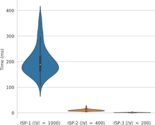
The performance of BEST2COP being already promising on non-advantageous scenarios, we now analyze its performance in realistic cases. Our basic settings are left unchanged, i.e., Γ = 1000 and BEST2COP still does not take advantage of any distance pruning to reduce G′. We first evaluate BEST2COP’s execution times on a large network topology with real IGP weights but random delays. Then, we consider real but smaller network structures having both real IGP weights and delays. Our goal is to show at which extent BEST2COPcan benefit from concrete network characteristics, making it efficient enough to be deployable for real-life cases. The first ISP, ISP1, consists of more than 1100 nodes and 3000 edges. While we do possess the IGP costs of each link in E, we do not have their delays. Thus, we select random values and set them directly on E (and not on E′as in the previous evaluation). More precisely, we consider here a maximum delay leading to the worst experimental computing time, which is 70. We then also consider two other real ISP networks, ISP2 and ISP3, with respectively around 400 and 200 nodes, having real valuations for M1 and M2. The execution time results are

shown in Fig. 5 as violin plots, whose widths represent the number of executions taking the time shown on the y-axis (in ms). We run BEST2COP for all sources.

BEST2COP clearly benefits from ground graph properties. Its execution time rarely exceeds 250ms in the most dis-advantageous experiments on ISP1. For ISP2 and ISP3, the computing is almost negligible, mostly because∣V ∣ is limited. The execution times were greatly enhanced thanks to the realistic network structures and weights leading to small Pareto fronts (few distances dominate all the others because metrics are often aligned). Even though the delay is still random for ISP1, simply using a realistic network structure divided the execution time by two when compared to a randomly-weighted full-mesh of similar size (see Fig. 4). BEST2COP already

ISP-1 (|V| 1000) ISP-2 (|V| 400) ISP-3 (|V| 200) 0 100 200 300 400 Time (ms)

Figure 5: BEST2COP’s performances on realistic topologies with realistic weights (but random delays for ISP1). Execution times remain mostly under 100ms, even though some of the delays are still randomized for ISP1.

shows great improvements regarding its execution time on ISP1, although it does not benefit from real-life delays as in ISP2 and ISP3. In such cases with few nodes, BEST2COP solves 2COP in a negligible amount of time. In realistic cases, it seems thus possible to increase Γ to reach a delay accuracy on the order of the micro-second while keeping the execution time in the hundreds of milliseconds.

V. RELATEDWORK

QoS routing and TE being popular subjects for several years, it is impossible to showcase here all past work. How-ever, there are several extensive surveys [1], [12], [13] that exhibit a lot of the solutions developed in the past decades.

Specific to DCLC, DCUR [14] explores the network by extending paths either through the delay or the least-cost path. DCUR has been combined with Bellman-Ford to create DCBF [15], which guesses promising paths through an estimated cost. Closer to our work, Constrained Bellman-Ford [16], solves DCLC exactly by exploring paths in a greedy fashion through a priority queue indexed on their delay. CBF was extended in [17], which adds two heuristics to ease the problem, first by discretizing all metrics but one, second by only extending k best paths.

Segment Routing also attracted a lot of interest from the research community, as can be seen in [18]. While some SR-TE works are centered around the constrained paths prob-lem [19], [20], most of the work related to SR does not focus on DCLC, but rather bandwidth optimization [21], [22], path encoding [23], [24], or network resiliency [25], [26]. In addition, they usually rely on complex parametrizable techniques such as constraint programming or ILP which may lead to high computation times [18]. Some works do however use a construct similar to ours in order to prevent the need to perform conversions from network paths to segment lists. [27], in particular, proposes a multi-metric construct that does not however take advantage of dominated segments. In addition, they do not aim to solve DCLC, but simply use the construct to discover paths before sorting them lexicographically.

©IEEE, 2020. This is the author’s version of an article that has been published in the NCA conference. Changes were made to this version by the publisher prior to publication.

We propose an all-in-one solution, that solves 2COP and returns the corresponding list of segments. Our approach is an exact algorithm with a straight-forward bounded worst-case time complexity, with no parameters requiring tuning. While other works solving DCLC usually detach path computations and their deployment, we are, to the best of our knowledge, the first ones to propose an algorithm that leverages SR deployment constraints to solve DCLC for SR. In addition, while not all works evaluate the time complexity of their solution, or do so on limited topologies, we provide extensive evaluations on random and real large topologies, bounding the worst-case time complexity of BEST2COP.

VI. CONCLUSION

While the management overhead of MPLS-based solutions leads to a TE winter in the past decade, Segment Routing marked its rebirth. In particular, SR enables the deployment of a practical solution to the well-known DCLC problem. In this paper, we proposed an efficient multi-metric SR con-struct onto which our algorithm, BEST2COP, iterates to solve DCLC in SR domains. Relying on adaptive simple structures, BEST2COP leverages both an SR operational constraint and the inherent limited accuracy of measured delays. By natively encompassing such limits, we efficiently handle all scenarios. Through extensive evaluation, we showed that BEST2COP performs well with both random and realistic cases.

While we believe BEST2COP is already efficient enough to be deployed, several improvements are possible to make it even more scalable. First, its parallelizable nature and smart strategies for cache reuse can be exploited. Similarly, to deal with really high trueness requirements, more advanced, and flexible structures can be envisioned. Finally, for large ISPs relying on subdivision in areas, partitioning DCLC into smaller sub-problems seems promising to further reduce the complexity of BEST2COP.

ACKNOWLEDGEMENTS

This work was partially supported by the French National Research Agency (ANR) project Nano-Net under contract ANR-18-CE25-0003.

REFERENCES

[1] F. Kuipers, P. Van Mieghem, T. Korkmaz, and M. Krunz, “An overview of constraint-based path selection algorithms for qos routing,” IEEE Communications Magazine, vol. 40, no. 12, pp. 50–55, 2002. [2] Zheng Wang and J. Crowcroft, “Quality-of-service routing for

sup-porting multimedia applications,” IEEE Journal on Selected Areas in Communications, vol. 14, no. 7, pp. 1228–1234, 1996.

[3] S. Chen and K. Nahrstedt, “On finding multi-constrained paths,” vol. 2, 07 1998, pp. 874 – 879 vol.2.

[4] S. Shalunov, B. Teitelbaum, A. Karp, J. Boote, and M. Zekauskas, “A one-way active measurement protocol (owamp),” Internet Requests for Comments, RFC Editor, RFC 4656, September 2006.

[5] K. Hedayat, R. Krzanowski, A. Morton, K. Yum, and J. Babiarz, “A two-way active measurement protocol (twamp),” Internet Requests for Comments, RFC Editor, RFC 5357, October 2008.

[6] ISO, “Accuracy (trueness and precision) of measurement methods and results — Part 1: General principles and definitions,” International Or-ganization for Standardization, Geneva, Switzerland, ISO 5725-1:1994, 1994.

[7] G. Almes, S. Kalidindi, M. Zekauskas, and A. Morton, “A one-way delay metric for ip performance metrics (ippm),” Internet Requests for Comments, RFC Editor, STD 81, January 2016.

[8] G. Almes, S. Kalidindi, and M. Zekauskas, “A round-trip delay metric for ippm,” Internet Requests for Comments, RFC Editor, RFC 2681, September 1999.

[9] C. Filsfils, N. K. Nainar, C. Pignataro, J. C. Cardona, and P. Francois, “The segment routing architecture,” in 2015 IEEE Global Communica-tions Conference (GLOBECOM), 2015, pp. 1–6.

[10] A. Farrel, J.-P. Vasseur, and J. Ash, “A path computation element (pce)-based architecture,” Internet Requests for Comments, RFC Editor, RFC 4655, August 2006.

[11] M. Garey and D. Johnson, “Computers and intractability–a guide to np-completeness.(1979).”

[12] J. W. Guck, A. V. Bemten, M. Reisslein, and W. Kellerer, “Unicast qos routing algorithms for sdn: A comprehensive survey and performance evaluation,” IEEE Communications Surveys & Tutorials, vol. 20, pp. 388–415, 2018.

[13] R. G. Garroppo, S. Giordano, and L. Tavanti, “A survey on multi-constrained optimal path computation: Exact and approximate algo-rithms,” Computer Networks, vol. 54, no. 17, pp. 3081 – 3107, 2010. [14] D. S. Reeves and H. F. Salama, “A distributed algorithm for

delay-constrained unicast routing,” IEEE/ACM Transactions on Networking, vol. 8, no. 2, pp. 239–250, 2000.

[15] Zhanfeng Jia and P. Varaiya, “Heuristic methods for delay constrained least cost routing using /spl kappa/-shortest-paths,” IEEE Transactions on Automatic Control, vol. 51, no. 4, pp. 707–712, 2006.

[16] R. Widyono and T. Group, “The design and evaluation of routing algorithms for real-time channels,” 1994.

[17] Xin Yuan and Xingming Liu, “Heuristic algorithms for multi-constrained quality of service routing,” in Proceedings IEEE INFOCOM 2001. Conference on Computer Communications. Twentieth Annual Joint Conference of the IEEE Computer and Communications Society (Cat. No.01CH37213), vol. 2, 2001, pp. 844–853 vol.2.

[18] P. L. Ventre, S. Salsano, M. Polverini, A. Cianfrani, A. Abdelsalam, C. Filsfils, P. Camarillo, and F. Clad, “Segment Routing: a Com-prehensive Survey of Research Activities, Standardization Efforts and Implementation Results,” arXiv:1904.03471 [cs], Jul. 2020, arXiv: 1904.03471.

[19] X. Hou, M. Wu, and M. Zhao, “An optimization routing algorithm based on segment routing in software-defined networks,” Sensors, vol. 19, p. 49, 12 2018.

[20] R. Hartert, P. Schaus, S. Vissicchio, and O. Bonaventure, “Solving seg-ment routing problems with hybrid constraint programming techniques,” in Principles and Practice of Constraint Programming, G. Pesant, Ed. Cham: Springer International Publishing, 2015, pp. 592–608. [21] R. Bhatia, F. Hao, M. Kodialam, and T. V. Lakshman, “Optimized

network traffic engineering using segment routing,” in 2015 IEEE Conference on Computer Communications (INFOCOM), 2015, pp. 657– 665.

[22] S. Gay, R. Hartert, and S. Vissicchio, “Expect the unexpected: Sub-second optimization for segment routing,” IEEE INFOCOM 2017 - IEEE Conference on Computer Communications, pp. 1–9, 2017.

[23] R. Guedrez, O. Dugeon, S. Lahoud, and G. Texier, “Label encoding algorithm for mpls segment routing,” in 2016 IEEE 15th International Symposium on Network Computing and Applications (NCA). IEEE, pp. 113–117.

[24] A. Giorgetti, P. Castoldi, F. Cugini, J. Nijhof, F. Lazzeri, and G. Bruno, “Path encoding in segment routing,” in 2015 IEEE Global Communica-tions Conference (GLOBECOM), 2015, pp. 1–6.

[25] K. Foerster, M. Parham, M. Chiesa, and S. Schmid, “Ti-mfa: Keep calm and reroute segments fast,” in IEEE INFOCOM 2018 - IEEE Conference on Computer Communications Workshops (INFOCOM WKSHPS), 2018, pp. 415–420.

[26] F. Hao, M. Kodialam, and T. V. Lakshman, “Optimizing restoration with segment routing,” in IEEE INFOCOM 2016 - The 35th Annual IEEE International Conference on Computer Communications, 2016, pp. 1–9. [27] F. Lazzeri, G. Bruno, J. Nijhof, A. Giorgetti, and P. Castoldi, “Efficient label encoding in segment-routing enabled optical networks,” 2015 International Conference on Optical Network Design and Modeling (ONDM), pp. 34–38, 2015.