A coarse-mesh nodal diffusion method based on response matrix considerations

NUCLEAR ENGINEERING

READING ROM

-

M.I.T.

A COARSE-MESH NODAL

DIFFUSION

METHOD

BASED ON

RESPONSE MATRIX CONSIllERATIONS

BY

ALLAN

F.

HENRY, RANDAL

N.

SIMS

MARCH

1977

DEPARTMENT OF NUCLEAR ENGINEERING MASSACHUSETTS INSTITUTE OF TECHNOLOGY

CAMBRIDGE, MASSACHUSETTS

02139

A COARSE-MESH NODAL DIFFUSION METHOD BASED ON RESPONSE MATRIX CONSIDERATIONS

NUCLEI

7

NERING

READING

M.I.T.

by

Allan F. Henry, Randal N. Sims

March 1977

Department of Nuclear Engineering Massachusetts Institute of Technology

Cambridge, Massachusetts 01293

A COARSE-MESH NODAL DIFFUSION METHOD BASED ON RESPONSE MATRIX CONSIDERATIONS

by

Randal Nee Sims

Submitted to the Department of Nuclear Engineering on March 11, 1976, in partial fulfillment of the

requirements for the Degree of Doctor of Science

ABSTRACT

The overall objective of this thesis is to develop an economical computational method for multidimensional transient analysis of nuclear power reactors. Specifically, the application of nodal methods based on the multigroup diffusion theory approximation to reactors composed of regular arrays of large homogeneous (or homogenized) zones was investigated.

A nodal scheme is formulated using the response matrix approach as a conceptual basis. Solutions of equivalent sets of coupled

one-dimensional problems are used to treat the local multione-dimensional re-sponse problems. Polynomial expansions in conjunction with weighted residual procedures are employed to obtain approximate solutions of the one-dimensional problems. A linear set of nodal equations express-ed in terms of nodal average fluxes and interface average partial cur-rents is obtained.

Applications to two-dimensional few-group, static and transient problems demonstrate that the nodal scheme can be an order of mag-nitude more computationally efficient than conventional finite differ-ence methods.

Thesis Supervisor: Allan F. Henry Title: Professor of Nuclear Engineering

TABLE OF CONTENTS ABSTRACT LIST OF FIGURES LIST OF TABLES ACKNOWLEDGMENTS BIOGRAPHICAL NOTE Chapter 1. INTRODUCTION 1.1 Overview

1.2 Statement of the Problem

1.3 General Review of Solution Techniques

1.4 Nodal Method Development - Motivation and Objectives

1.5 Summary

Chapter 2. DERIVATION OF THE SPATIALLY-DISCRETIZED TIME-DEPENDENT NODAL EQUATIONS

2.1 Introduction

2.2 Motivation

2.2.1 A Response Matrix Viewpoint 2.2.2 Reduction of the Multidimensional

Problem to an Equivalent Coupled Set of One-dimensional Problems

Page 2 8 11 13 14 15 15 16 19 22 22 24 24 25 25 27

2.3 Derivation in Two-dimensional Cartesian

Geometry with Uniform Nodal Properties and a General Energy Group Structure

2.3.1 Formulation of the Coupled Set of One-dimensional Problems

2.3.2 Restraints Imposed on the Solution 2.3.3 Approximate Solution

2.3.3.1 Choice of Approximating Functions

2.3.3.1a One-dimensional Average

Fluxes

2.3.3.1b One-dimensional Average

Delayed Precursors 2.3.3.lc Transverse Leakage

2.3.3.2 Weighted Residual Procedure 2.3.3.3 Final Form

2.4 Relationship to Other Work

2.5 Summary

Chapter 3. STATIC APPLICATIONS

3.1 Introduction

3.2 Reduction of the Spatially-Discretized,

Time-Dependent Nodal Equations to the Static Case

3.3 Numerical Solution of the Static Eigenvalue

Problem

3.3.1 General Formulation

3.3.2 Fission Source Iterations

29 29 31 33 33 33 35 36 39 40 45 46 47 47 47 50 50 51

3.3.3 Within-Group Spatial Solutions 3.3.3.1 Flux Condensation

3.3.3.2 Solution in One Dimension 3.3.3.3 Solution in Two Dimensions

3.3.3.3.1 Inner Iterations

3.3.3.3.2 The "Row-Column" Block

Iterative Method

3.3.3.3.3 The "Response Matrix"

Block Iterative Method

3.3.3.3.4 Comparison of the

Numer-ical and Computational Aspects of the Proposed Block Iterative Schemes 3.3.3.4 Extension to Three Dimensions

Page 53 53 55 56 56 58 61 69 71 72 74 74 75 75 77 80 82 82 3.3.4 Computer Codes - Applications and

Comparisons

3.4 Results

3.4.1 Foreword

3.4.2 One Dimension

3.4.2.1 Kang's One-dimensional LWR Problem

3.4.2.2 A One-dimensional Version of the IAEA PWR Problem

3.4.2.3 Summary of One-dimensional Results

3.4.3 Two Dimensions

3.4.3.1 Comparison of Iterative Schemes for the Inner Iterations

3.4.3.2 The IAEA Two-dimensional PWR Benchmark Problem

3.4.3.3 The LRA Two-dimensional BWR Benchmark Problem

3.4.3.4 The Biblis PWR Problem 3.4.3.5 Summary of Two -dimensional

Results

3.5 Summary

4. TRANSIENT APPLICATIONS 4.1 Introduction

4.2 Discretization in Time

4.3 Solution of the Discrete Time-Dependent Equations 4.3.1 Problem Formulation

4.3.2 Solution Method

4.3.3 Numerical Considerations

4.4 Results

4.4.1 The TWIGL Two-dimensional Seed-Blanket Reactor Problem

4.4.2 The LRA Two-dimensional BWR Benchmark Problem

4.5 Summary

SUMMARY

Overview of Thesis Results

Recommendations for Future Work Chapter 5. 5.1 5.2 Page 89 95 97 Chapter 100 101 103 103 104 108 108 109 111 114 114 132 146 148 148 150

REFERENCES Appendix 1. Appendix 2. Appendix 3. Appendix 4. Appendix 5.

ONE-DIMENSIONAL AVERAGE FLUX EXPANSION FUNCTIONS

"QUADRATIC" TRANSVERSE LEAKAGE EXPANSION FUNCTIONS

WEIGHT FUNCTIONS

EVALUATION OF WEIGHTED INTEGRALS DESCRIPTIONS OF TEST PROBLEMS

A5.1 Kang' s One-dimensional LWR Problem

A5.2 A One-dimensional Version of the IAEA PWR Problem

A5.3 The IAEA Two-dimensional PWR Benchmark Problem

A5.4 The LRA Two-dimensional BWR Benchmark Problem

A5.5 The Biblis Two-dimensional PWR Problem A5.6 The TWIGL Two-dimensional Seed-Blanket

Reactor Problem

Appendix 6. RESULTS

A6.1 Kang' s One-dimensional LWR Problem

A6.2 A One-dimensional Version of the IAEA PWR Problem

A6.3 The IAEA Two-dimensional PWR Benchmark Problem

A6.4 The LRA Two-dimensional BWR Static Benchmark Problem Page 152 156 163 168 171 175 176 177 178 180 184 185 188 189 192 194 197

Page

A6.5 The TWIGL Two-dimensional Seed-Blanket

Reactor Problem 198

A6.6 The LRA Two-dimensional BWR Kinetics

LIST OF FIGURES

No. Page

Al. 1 Basis Functions for the One-dimensional Average

Flux Equations 160

A2. 1 Basis Functions for the Quadratic Transverse Leakage

Expansion 167

A3. 1 Weight Functions for the One-dimensional Weighted

Residual Procedure 170

A6. la Thermal Flux Plot for Kang's One-dimensional LWR

Problem: 20 cm Mesh 189

A6. lb Thermal Flux Plot for Kang's One-dimensional LWR

Problem: 10 cm Mesh 190

A6. lc Thermal Flux Plot for Kang's One-dimensional LWR

Problem: 5 crp Mesh 191

A6. 2a Power Distribution for the One-dimensional IAEA PWR Problem: Results of Uniform Mesh

Refine-ment 192

A6. 2b Power Distribution for the One-dimensional IAEA

PWR Problem: Refinement of Reflector Treatment 193

A6. 3a Power Distribution for the Two-dimensional IAEA PWR Problem (Regular Core): Results of Uniform Mesh Refinement with the Constant Transverse

Leakage Approximation 194

A6. 3b Power Distribution for the Two-dimensional IAEA PWR Problem (Regular Core): Results of Uniform Mesh Refinement with the Quadratic Transverse

Leakage Approximation 195

A6. 3c Power Distribution for the Two-dimensional IAEA PWR Problem (Irregular Core): Coarse Mesh

Results 196

A6. 4 Power Distribution for the LRA BWR Static

Prob-lem (Rods Inserted): Coarse Mesh Resuits 197

A6. 5a Static Power Distribution Results for the TWIGL

No. _Page

A6. 5b Asymptotic Power Distribution Results for the TWIGL

Two-dimensional Seed-Blanket Reactor Problem 199 A6. 5c _{Reactor Power versus Time for the TWIGL}

Two-dimensional Seed-Blanket Reactor Problem (Step

Perturbation) 200

A6. 5d _{Reactor Power versus Time for the TWIGL} Two-dimensional Seed-Blanket Reactor Problem (Ramp

Perturbation) 201

A6. 5e Iterations versus Timestep for the TWIGL Two-dimensional Seed-Blanket Reactor Problem (Step

Perturbation): Very Coarse Mesh 202

A6. 5f _{Iterations versus Timestep for the TWIGL} Two-dimensional Seed-Blanket Reactor Problem (Step

Perturbation): Coarse Mesh 203

A6. 5g Iterations versus Timestep for the TWIGL Two-dimensional Seed-Blanket Reactor Problem (Ramp

Perturbation): Very Coarse Mesh 204

A6. 5h _{Iterations versus Timestep for the TWIGL} Two-dimensional Seed-Blanket Reactor Problem (Ramp

Perturbation): Coarse Mesh 205

A6. 6a Power Distribution for the LRA BWR Static Prob-lem (Rods Inserted): Very Coarse Mesh Results with

the Quadratic Transverse Leakage Approximation 206 A6. 6b Power Distribution for the LRA BWR Static

Prob-lem (Rods Withdrawn): Very Coarse Mesh Results with the Quadratic Transverse Leakage

Approxi-mation 207

A6.6c Power versus Time for the LRA Two-dimensional

BWR Kinetics Benchmark Problem 208

A6. 6d Temperature versus Time for the LRA

Two-dimensional BWR Kinetics Benchmark Problem 210

A6.6e Power and Temperature Distributions for the LRA

BWR Kinetics Benchmark Problem at Time = 0. 0 sec 211 A6.6f Power and Temperature Distributions for the LRA

No. Page

A6.6g Power and Temperature Distributions for the LRA

BWR Kinetics Benchmark Problem at Time = 2. 00 sec 213 A6.6h Power and Temperature Distributions for the LRA

BWR Kinetics Benchmark Problem at Time = 3. 00 sec 214 A6.6i Iterations versus Timestep for the LRA

Two-dimensional BWR Kinetics Benchmark Problem:

First Time Domain 215

A6. 6j Iterations versus Timestep for the LRA Two-dimensional BWR Kinetics Benchmark Problem:

Second Time Domain 216

A6.6k Iterations versus Timestep for the LRA Two-dimensional BWR Kinetics Benchmark Problem:

Third Time Domain 218

A6. 61 Iterations versus Timestep for the LRA Two-dimensional BWR Kinetics Benchmark Problem:

Fourth Time Domain 220

A6.6m Iterations versus Timestep for the LRA Two-dimensional BWR Kinetics Benchmark Problem:

Fifth Time Domain 222

A6. 6n Iterations versus Timestep for the LRA Two-dimensional BWR Kinetics Benchmark Problem:

LIST OF TABLES

No. _Page

3. 1 Results for Kang's One-dimensional LWR Problem 76 3. 2 Summary of Results for the One-dimensional Version

of the IAEA PWR Problem: Uniform Mesh Refinement 79 3. 3 _{Summary of Results for the One-dimensional Version}

of the IAEA PWR Problem: Improved Reflector

Treat-ment 81

3. 4 _{Comparison of Iterative Solution Methods Applied to}

the IAEA Two-dimensional PWR Benchmark Problem 84 3. 5 Summary of Finite Difference Results for the IAEA

Two-dimensional PWR Benchmark Problem 90 3. 6 Summary of Results for the IAEA Two-dimensional

PWR Benchmark Problem (Regular Core) 91

3. 7 Summary of Results for the IAEA Two-dimensional

PWR Benchmark Problem (Irregular Core) 94 3. 8 Summary of Results for the LRA Two-dimensional

Static BWR Benchmark Problem 96

3. 9 Summary of Results for the Biblis Two-dimensional

PWR Problem (Rods Withdrawn) 98

3. 10 Summary of Results for the Biblis Two-dimensional

PWR Problem (Rods Inserted) 99

4. 1 Summary of Static Results for the TWIGL

Two-dimensional Seed-Blanket Reactor Problem 116 4. 2 Total Power versus Time for the TWIGL

Two-dimensional Seed-Blanket Reactor (Step Per-turbation): Investigation of the Spatial Iteration

Convergence Criterion 118

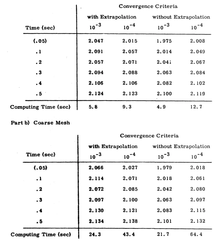
4. 3 _{Total Power versus Time for the TWIGL} Two-dimensional Seed-Blanket Reactor Problem (Step Perturbation): Investigation of the Effects of

No. Page

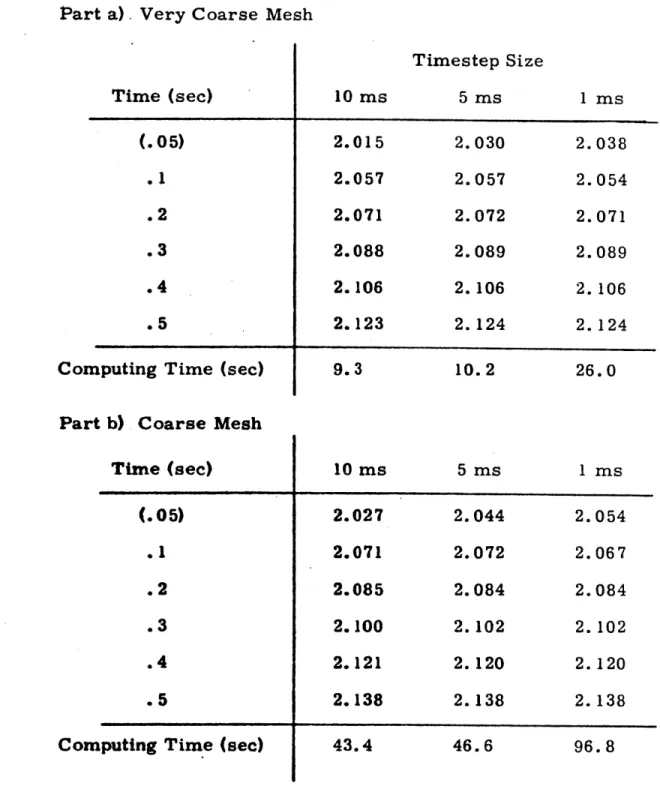
4. 4 Total Power versus Time for the TWIGL Two-dimensional Seed-Blanket Reactor Problem (Step Perturbation): Investigation of Temporal

Conver-gence for the Constant Transverse Leakage

Approx-imation 122

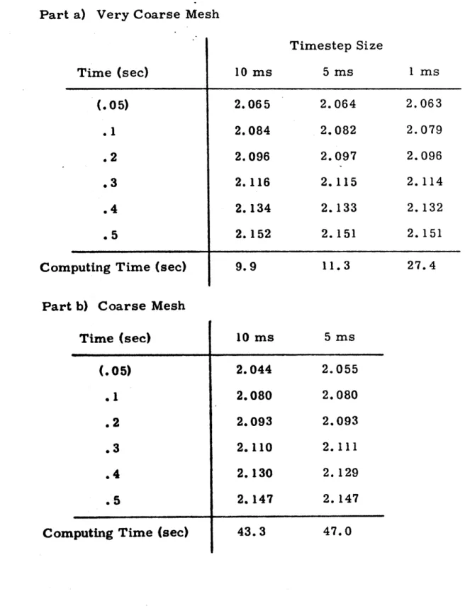
4. 5 Total Power versus Time for the TWIGL Two-dimensional Seed-Blanket Reactor Problem (Step Perturbation): Investigation of Temporal

Conver-gence for the Quadratic Transverse Leakage

Approximation 123

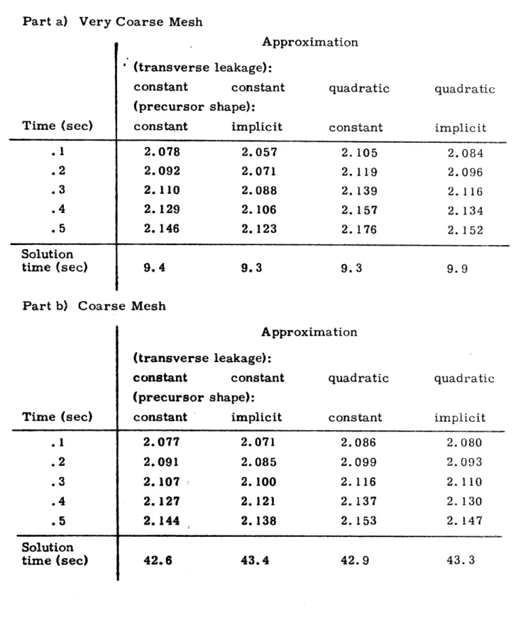
4. 6 Total Power versus Time for the TWIGL Two-dimensional Seed-Blanket Reactor Problem (Step

Perturbation): Comparison of Transverse Leakage

and Precursor Shape Approximations 126

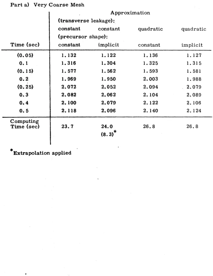
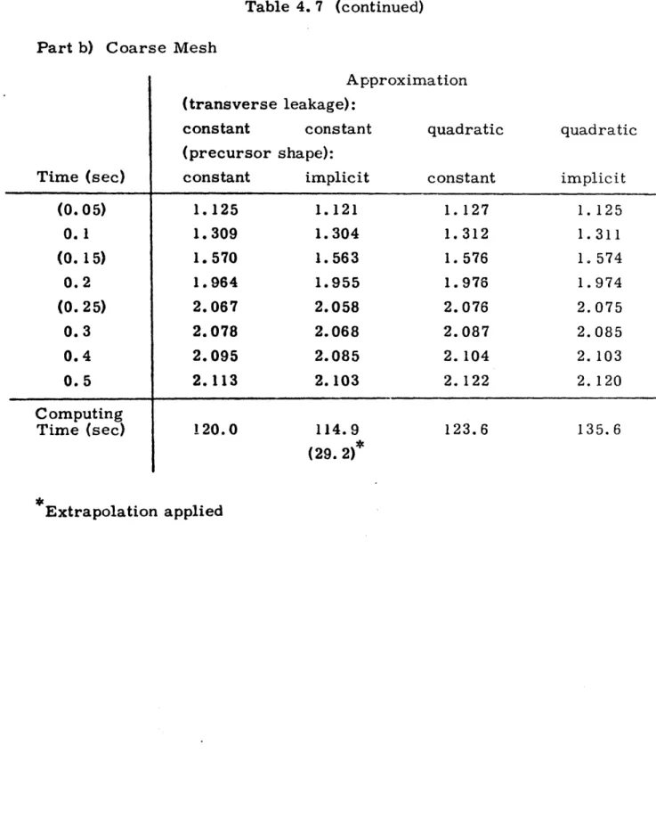
4. 7 Total Power versus Time for the TWIGL Two-dimensional Seed-Blanket Reactor Problem (Ramp Perturbation): Comparison of Transverse

Leak-age and Precursor Shape Approximations 127 4. 8 Summary of Results for the TWIGL Two-dimensional

Seed-Blanket Reactor Problems 129

4. 9 Summary of Static Results for the LRA Two-dimensional BWR Benchmark Problem: Very

Coarse Mesh 135

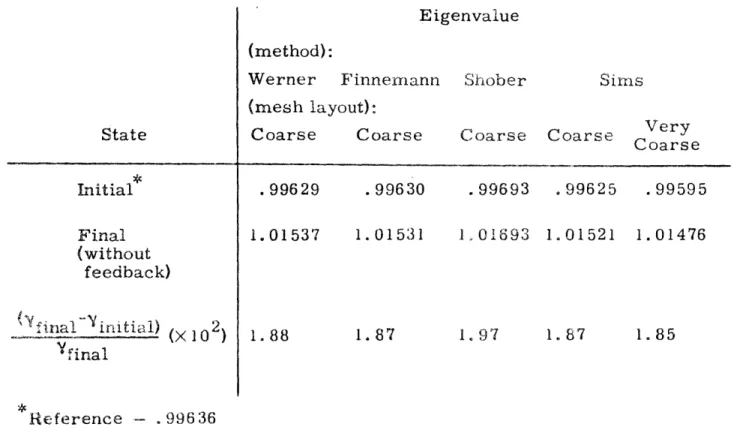
4. 10 Static Eigenvalues for the Initial State and Final State (without Feedback) of the LRA Two-dimensional BWR

Kinetics Benchmark Problem 136

4. 11 Summary of Results for the LRA Two-dimensional

BWR Kinetics Benchmark Problem 140

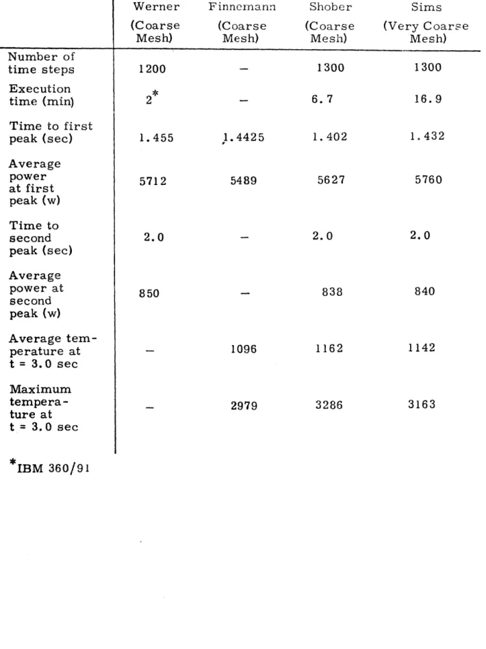
4. 12 Summary of Computational Results for the LRA

ACKNOWLEDGMENTS

The author expresses his sincerest appreciation to his thesis

super-visor, Professor Allan F. Henry, for his guidance, encouragement, and support throughout the course of this thesis work. It has been a pleasure,

as well as an extremely rewarding experience, to be associated with

him during the author's stay at M. I. T.

The financial support of this research by the Electric Power

Re-search Institute is gratefully acknowledged.

All computation was performed on an IBM 370/168 computer at the MIT Information Processing Center.

The author also thanks Mrs. Esther Grande for her skill, care,

BIOGRAPHICAL NOTE

Randal Nee Sims was born August 13, 1950 in Dyer, Tennessee.

He attended elementary and secondary school in Dyer, Tennessee, and

received a high school diploma in May, 1968.

He enrolled in the University of Tennessee at Martin in June, 1969.

There he began participation in the industry-university cooperative

program with his work experience carried out at the DuPont Savannah

River Plant and Laboratory in Aiken, South Carolina. After transfer

to the University of Tennessee at Knoxville in March, 1971, he received

the degree of Bachelor of Science in Engineering Physics in June, 1973.

In September, 1973, he entered the Massachusetts Institute of

Tech-nology as a graduate student in the Department of Nuclear Engineering.

While at M. I. T., his association with the Savannah River Plant and

Laboratory continued through participation in their summer graduate

Chapter 1

INTRODUCTION

1. 1 Overview

There exists a strong economic incentive to perform accurate,

reli-able, and reasonably inexpensive multidimensional static and transient

reactor calculations. The accurate prediction of multidimensional

reac-tor behavior can lead to direct gains in terms of an increase in operating

efficiency and reactor utilization or more indirect benefits such as a

relaxation of safety margins or an increased confidence in their

relia-bility.

The standard computational technique for power distribution

calcula-tions in full-size reactors is the finite difference method. However, the

limited spatial accuracy of the method with the corresponding necessity

for excessive spatial discretization place severe demands on computer

resources. Thus, only recently, with the development of new

computa-tional procedures and a dramatic improvement in computer technology,

have three-dimensional finite -difference static calculations been

under-taken on a routine basis. Moreover, accurate multidimensional modeling

using finite difference techniques of realistic transients for the large

power reactors currently being built and designed is prohibitively

expen-sive.

A number of recently developed higher order computational schemes have been demonstrated to be efficient alternatives to the finite

differ-ence method for multidimensional static calculations. For a comprehensive

the requirements of multidimensional static and dynamic calculations

and the development of computational methods to meet those needs.1-6

In particular, nodal techniques have reached a high degree of

sophistica-tion in applicasophistica-tion to static. problems.5 This demonstrated success with

static nodal schemes has prompted us to investigate the various nodal

formulations with particular emphasis on developing a spatially accurate

and computationally efficient technique for transient calculations. Other

researchers have pursued this same approach.6

The overall objective of this thesis is to develop an economical

method for transient analysis of nuclear power reactors. In particular,

nodal schemes for time-dependent analysis of light water reactors will be

investigated. However, the basic intent is to develop a method with

ade-quate generality to treat the principal reactor types currently under design.

1. 2 Statement of the Problem

It is generally assumed that multigroup diffusion theory is an

accep-tably accurate neutronics model for the prediction of detailed reactor

behavior. Thus the basic set of time- and spatially-dependent

equa-tions for which we shall discuss approximate soluequa-tions are

- D (r, t) V4 (r, t) - Erg (r, t) 4 (r, t) G + 6 Eg, (r, t) + (I-P) X , (r, t) g , (r, t) gK=1 + I XgkCk(r, t) =

+

G =8 k T, v Tfg(rt) g(r, t) - XkCk(r,t) =

Ck(r,

G = total number of neutron energy groups K total number of delayed precursor families

-2 -1 4) neutron flux in group g (cm sec )

g

Ck density of delayed precursor in family k (cm- 3

Dg diffusion coefficient for group g (cm)

-1 M rg macroscopic removal cross section for group g (cm )

rg

1 ,9 amacroscopic transfer cross section from group g' to

gg r -1 group g (cm ) 6 g* g'48

0

Li

P total fractional yield of delayed precursors per fission X g prompt fission spectrum for group g

g

v athe number of neutrons per fission divided by a normalizing y rg

parameter which is adjusted to establish a steady-state condition for the reactor with time-independent properties times the macroscopic fission cross section for group g (cm~ )

Xgk delayed spectrum for family k to group g

xk decay constant for family k

and the implicit assumption has been made that only one fissionable isotope is present. Stated nonmathematically, the particular boundary conditions imposed are that the solution of Eq. (1. 1) be restrained to equal zero on the reactor boundary or be such that the reactor is effec-tively imbedded in a vacuum. At internal interfaces, continuity of the flux and normal component of the neutron current are required. For the reactor with time-independent properties, the static solution (or initial condition for the time-dependent Eq. (1. 1)) is obtained effectively by varying the parameter y until all time derivatives vanish for any arbitrary initial condition. The static equations are

9 (r) V4 (r) - E (r) 9 (r)

- g- -g-- rg-

g-G

+gi ( , g ,(r) + xI Y2 fgI(r) 4g,(r) =0; g = 1,2,.. .G. (1. 2) The geometrical complexity of most large power reactors is so great

that it is generally impractical to treat the spatial detail directly. To

alleviate this difficulty, prescriptions have been developed for obtaining

equivalent homogenized diffusion theory parameters which are spatially

constant over relatively large reactor regions (for instance, the size

of a single fuel assembly in the radial plane). Thus the global reactor

problem is normally partitioned into an array of subregions with constant

material properties and typically uniform geometric properties. This

1. 3 General Review of Solution Techniques

Among the most successful of methods for solution of static

multi-dimensional problems, Eq. (1. 2), are finite difference, finite element,

synthesis, and nodal techniques. We cannot adequately detail each of

these approaches here and therefore refer the reader to the

comprehen-sive reviews previously mentioned. 3,5 We merely summarize the

advan-tages and faults of each general class.

The finite difference method 8,9 is based on nodewise integral

neu-tron balance with a low-order difference approximation used to represent

spatial integrals of the leakage term V - D (r) V4) (r). The resulting

equations are sparsely coupled in space and energy making them

rela-tively easy to solve. The spatial coupling is of the "nearest neighbor"

type, meaning that only adjacent nodes are coupled in the representation

of the spatial leakage terms. Powerful numerical solution techniques

using sophisticated iterative strategies have been developed for systems

of equations with this particular type of structure.10 1 2 Also, it can

be shown that the finite difference method converges to the exact

solu-tion of the multigroup diffusion equasolu-tions in the limit of vanishing node

size. However, the finite difference method applied to the "homogenized"

problem has been found to require an excessive number of unknowns to 3

achieve adequate accuracy. Nevertheless, because of the inherent

simplicity and reliability of the method, it is the industry standard for

full-scale reactor analysis, and accordingly, the one to which we shall

compare our schemes.

for approximation of the detailed spatial variables. Variational proce-dures are applied to determine the unknown polynomial coefficients. The use of high-order spatial approximations allows a substantial reduction in the number of unknowns in relation to the finite difference method to achieve comparable spatial accuracy. Convergence to the exact solution of the multigroup diffusion equations in the limit of vanishing mesh size can be shown. However, the coupling of the unknowns in the finite ele-ment equations is much less sparse than that of the finite difference method, and because of this complexity, the advantage in computational efficiency of the finite element method is severely limited.5

The synthesis schemes7, 15 employ variational procedures using precomputed "trial functions" applicable over large regions of the reac-tor, such as two-dimensional planes, modulated by unknown coefficients with a reduced spatial dependence. This method can be used to treat the full spatial detail of the heterogeneous reactor with a vastly reduced number of unknowns compared with other more direct procedures. How-ever, the solution accuracy is dependent on a proper choice by the user of the trial functions. Moreover, systematic error bounds have not been established. This lack of guaranteed reliability has severely lim-ited the use of synthesis methods, especially in cases where safety considerations are important.

Nodal methods are derived directly from integral neutron balances and relate integral quantities, such average fluxes and neutron currents, over relatively large spatial regions. Nodal equations can be obtained

directly from the transport equation and thus are not necessarily limited by the diffusion theory approximation. This class of methods

includes many variants which are described in a number of review articles. 5, 7, 16-19 Here we shall pursue in detail only the particular items which have immediate application to our problem.

One subset of the general class of nodal schemes uses a represen-tation of interface currents as well as nodal fluxes allowing a system of equations to be constructed with a nearest neighbor spatial coupling formulation. Nodal balance equations (neutron conservation equations

for individual subvolumes relating net nodal reaction rates and leakages

in terms of average fluxes and interface currents) identical in structure to those of the finite difference method can be obtained if spatial coupling

parameters specifying the relationship between fluxes of neighboring

nodes and interface currents are introduced. This nodal approach offers

the advantages of simply-structured equations and a substantial reduction

in the number of unknowns by using average parameters over large

re-gions. Nevertheless, its use has been severely restricted because of

difficulties in predicting accurate spatial coupling parameters.

Fortunately, there seems to be a way around this difficulty. Recent

work on interface current type nodal techniques using an averaged

solu-tion representasolu-tion which incorporates schemes for the self-generasolu-tion

of spatial coupling parameters as an integral part of the overall

calcula-tional procedure or which deal directly with the interface currents

has shown much promise for producing efficient methods for

multidi-mensional static calculations.5 In this thesis, we will pursue a nodal

scheme based on the interface currents approach in which the neutron

1. 4 Nodal Method Development - Motivations and Objectives

The recent success with the interface currents type of approach previously discussed prompts us to look further at this particular

vari-ant of the general class of nodal methods. In general, the prospect of

a substantial reduction in the number of unknowns obtained by dealing only with avarage quantities over large nodal volumes plus the formu-lation of the equations with a nearest neighbor spatial coupling scheme

seems quite advantageous. However, we feel that previously developed

nodal techniques based on a diffusion theory approach have not fully

exploited the strong conceptual basis underlying the interface currents

approach in conjunction with formulations in which only integral

quanti-ties are represented.

Our specific objective is to develop a nodal method for solution of

the "homogenized,'" time-dependent, multidimensional, multigroup

dif-fusion theory problem. We intend to use the conceptual basis provided

by the interface currents approach and maintain a formulation involving only integral quantities. We shall attempt to develop a linear method

without the introduction of auxiliary parameters not directly expressible

in terms of the integral quantities of interest, the nodal average fluxes

and interface average currents.

1. 5 Summary

This thesis will be concerned with the development of

computation-ally efficient nodal methods for multidimensional transient analysis.

nodal equations is presented. Solution techniques and results are

dis-cussed for one- and two-dimensional

static

two-dimensional problems in Chapter 4. A summary of the investigation, a

statement of general conclusions, and recommendations for future work

Chapter 2

DERIVATION OF THE SPATIALLY-DISCRETIZED, TIME-DEPENDENT NODAL EQUATIONS 2. 1 Introduction

The derivation in the context of multigroup diffusion theory of a

multidimensional, spatially-discretized set of time-dependent equations

for the determination of average nodal fluxes is presented in this

chap-ter. In this formulation, only average quantities are represented and

a nearest neighbor spatial coupling scheme is preserved in the lowest

order linear approximation and in implied nonlinear higher order schemes.

Since the immediate goal in considering nodal schemes is the

replace-ment of the finite difference neutronics model in the pressurized (PWR)

and boiling (BWR) light water reactor transient analysis code MEKIN,

basic approximations pertaining to geometrical and material

represen-tations as used in that code are employed here. The assumption is made

in the MEKIN code that equivalent homogenized group parameters,

spa-tially constant over large nodal volumes, can be used to predict

ade-quately reactor transient behavior (see Sec. 1. 2). Therefore, only

Cartesian geometry and nodes having constant material properties are

considered. Also, for simplicity, only two dimensions are treated. The

reader should find the generalization to hexagonal geometry in two

dimensions (liquid metal fast breeder reactor, LMFBR) and

three-dimensional Cartesian (PWR, BWR) or hexagonal-axial (LMFBR)

geom-etry straightforward. Other researchers are investigating the

depletion studies for nodal schemes of the type presented here.21

2. 2 Motivation

2. 2. 1 A Response Mattix Viewpoint

It is well recognized that much of the trouble encountered in deter-mining spatial coupling parameters which predict accurate leakage rates based on the average fluxes alone of a node and its nearest neighbors is due to the fact that these parameters depend on the spatial detail of the fluxes and currents as well as on material and geometrical properties

of a node and its neighbors.5, 16 Difficulties obviously arise when an attempt is made to infer spatial coupling parameters predicting leakage

rates based on nearest neighbor average fluxes without some prior

knowledge of the true solution. However, until only recently, this has

been the conventional nodal approach.16

Basically, the difficulties are due to the fact that, in attempting to

use the nodal balance equation without auxiliary relations dealing either

with coupling parameters or with the nodal leakages themselves, an

incomplete system of equations is being used. For instance, the

pre-viously discussed interface current schemes have the nodal balance

equation as only one member of a coupled set that includes relations for

the interface leakages of a node expressed in terms of the leakage

cur-rents from neighboring nodes. Thus there is no reason to try to pursue

the idea of a single nodal balance equation with (necessarily nonlinear)

predetermined spatial coupling parameters to predict nodal leakage rates

A number of recently developed coarse-mesh diffusion methods employing variants of the interface currents approach in both linear and

nonlinear formulations have been demonstrated to be efficient

computa-tional techniques for multidimensional static calculations.5 (It should

be noted that we neglect the success of the sophisticated high-order

transport interface current approaches essentially because their

sophis-tication vastly exceeds the difficulty of our problem. 7) The similarity

of the nodal balance equations using nonlinear spatial coupling parameters

to the finite difference equations, for which well-established and powerful

solution procedures exist, have prompted some researchers to pursue

formulations in which the spatial coupling coefficients are generated in

auxiliary calculations included as an integral part of the overall

compu-tational procedure. 2 2-2 4 Others have used linear formulations of the

interface currents approach (linear in the sense that neutron currents

are treated directly) in low-order transport2 5 and diffusion theory

1 8_,2 6 _-3 1

approximations. In these efforts it is generally true that auxiliary

param-eters not directly expressible in terms of the average quantities of

interest (nodal fluxes and interface currents) or an explicit

representa-tion of the detailed spatial dependence of the solurepresenta-tion have been used in

order to achieve adequate spatial accuracy.

We follow the interface currents approach also. In particular, we

consider the response matrix method.18 However, we find that the

approximate solution can be restrained to a representation by average

quantities and a high-order spatial accuracy can be achieved without

the introduction of nonlinearities or auxiliary parameters not directly

nodal fluxes and interface currents).

The essential feature of the response matrix method is the deter-mination of reaction and leakage rates and distributions due to incident current boundary conditions with continuity of interface currents applied

to complete the global system of nodal equations. Application of this procedure results in a set of nodal equations with the advantageous fea-tures of local parameter determination (response parameters are only dependent on the properties of a single node) and nearest neighbor

cou-pling.

Of course, for practical application, this system must be discretized in terms of all the transport variables - angle, energy, and space. We work in the context of multigroup diffusion theory, so only the spatial dependence of the solution is of real concern (and the time dependence

for the transient problem). The treatment of the spatial dependence of

the nodal fluxes and interface currents is not a trivial matter, however,

especially since we desire to maintain a solution representation in terms

of average quantities only. This problem is discussed in the following

section.

2. 2. 2 Reduction of the Multidimensional Problem to an Equivalent Coupled Set of One-dimensional Problems

In order to pursue the response matrix procedure discussed in

Sec. 2. 2. 1, conceptually we must solve, using multigroup diffusion

theory, local multidimensional problems in homogeneous rectangular

nodes with time- and space-dependent incident current boundary

time- and space-dependent boundary leakage currents. For solution of

this problem, it is necessary to treat the spatial dependence of the nodal fluxes as well as the interface currents. However, since we want to minimize the number of unknowns by working only with average quanti-ties, we must find approximations for the spatial dependence of the nodal fluxes and interface currents in terms of the corresponding average

quantities. Alternatively, we can circumvent the problem by some trans-formation or reduction to q.n equivalent but more manageable system whose solution can be expressed in terms of average quantities. We employ both tactics.

We find that a high order of approximation can be achieved in the spatial solution of the local multidimensional response problem and the solution representation by average quantities only can be maintained, if

the multidimensional problem is reduced to a set of equivalent

one-dimensional problems by a straightforward spatial averaging procedure, and the spatial dependence of the unknowns in these equations are

approx-imated in terms of average quantities associated with each coordinate

direction. In particular, polynomial expansions which have coefficients

that can be interpreted as the average nodal fluxes and the interface

average currents associated with each coordinate direction are used for

approximation of the spatially-averaged one-dimensional fluxes. A

proper choice of polynomials allows a high-order approximation for the

one-dimensional average fluxes to be used without introducing auxiliary

parameters other than nodal average fluxes and interface average

appearing in the one-dimensional equations are expanded in polynomials

which have interface average currents as coefficients. A simple weighted

residual procedure is used to determine the unknown time-dependent

polynomial coefficients.

2. 3 Derivation in Two-dimensional Cartesian Geometry with Uniform Nodal Properties and a General Energy Group

Structure

2. 3. 1 Formulation of the Coupled Set of One-dimensional Problems

First, introduce the notational convention

u x,y; v y,x; v # u.

With x and y indicating the coordinate directions, u and v will be used

as coordinate subscripts. The global problem is subdivided into a regular

array of rectangular, nuclearly homogeneous regions. The partitioning

of the spatial domain is given by a grid defined by

u; =1, 2, .. L; u = x,y

where the following notation has been introduced for the grid indexing

urv,

1 1, 2, .... 1; u, v =x

j

Since we do not exclude the use of an irregular spatial domain,

there are a maximum of I X J nodes. For node (ij) defined by

y E [y , y ]

the node widths are defined as

h a l1-u; u = x, y and the node volume as

V.. - h h. 13 1 3

Now the multidimensional problem is reduced to an equivalent set of coupled one-dimensional equations by spatially averaging over the

direction transverse to each coordinate direction. For space direction u,

introduce the one-dimensional average neutron flux in energy group g

*u .. (u,t) 1 +1 dv c (u, v, t), (2.1) g,13L h _P. v_V

2 g

and the one-dimensional average delayed precursor density in delayed

family k

C U (u t) 1 +1 dv Ck(u, v, t). (2.2)

By spatially averaging Eqs. (1. 1) over each coordinate direction and inserting the definitions (2. 1) and (2. 2), the equivalent coupled set of

2

D _{A..) iju (u,} g, 13 u2 g, ij G + E g'=1 K + 1 k= 1 t) - Z ..(t) *u ..(u, t) - Lu ..(u, t) rg,ij g,ij g, ij

(

.. (t

)

u,

g,ij k k,13 a Cu .. (ut);t (k,ij k= 1, 2,_{U = X, y}

(2. 3b)

where L is the transverse leakage given by

h Lu .(u, t) = g, 13 D .. (t) h V V1 (a dv D . .t a 2 gE'j av2 a (u, vk,

+

2. 3. 2 Restraints Imposed on the Solution

For node (ij), define the nodal average flux for energy group g

) .(t)= 1 xi+1

g o ij _{V .. x} dx yj+1 yj

dy * (x, y, t) (2.5)

and the nodal average delayed precursor density for delayed family k

Ck, ij(t)

V

5j+1

It follows from the definition of the average one-dimensional fluxes and precursors, Eqs. (2. 1) and (2. 2), that

1 u+ _{du u .. (u, t) = M(t); u x,y} (2.7) hu g,1 g,ij and u l1 du Cu (u, t) Ck

j(t);

These relations, Eqs. (2. 7) and (2. 8), are just the formal statement

of a consistency condition that must be imposed on any approximate

solu-tion technique we employ. This consistency condisolu-tion states that, when averaged over the node, a one-dimensional average quantity must return the corresponding nodal average quantity.

Let us now consider the boundary conditions imposed on the

one-dimensional solutions. Because the delayed precursors are required to

obey no explicit boundary or interface continuity conditions, we need

only consider the one-dimensional average flux. It is easily seen that

the one-dimensional average flux obeys interface average incident

cur-rent boundary conditions. We define the interface average incident (in)

and leakage (out) partial currents by the normal diffusion theory relations7

inu-

(_U1

J u-(t) 1 u(u, t) - D . (t) u(u t) (2. 9a) g, 134 _{g, ij 2 g, i3 Ou g, ij}

u=u

Jout, u- M u (u,t) + D (t) 4u (u,t) (2. 9b) g, 1 _{4 g,13 2 go ij}

Jin, u+(t) . . u (u, t) + 1 D (t) *u (u,t) (2. 9c)

g,13 g, ij 2 g,ij au gij _n+1uu

Jou u(t) iu.(u, t) - D . (t) Iu . ( ). 2d

g, ij 4 g,13 2 g,1 ii u g,13 u=uf~

It is assumed that the J in's are the Jout's of neighboring nodes and thus are known by continuity in the solution of the local response problems.

The boundary conditions implicitly incorporated in the transverse

leakage terms, Eqs. (2. 3) and (2. 4), will not be discussed in detail at this time. As will be seen in a later discussion, the particular

high-order treatment used for the spatial dependence of the transverse leakage

is meaningful only in the context of the coupled global system of

equa-tions. However, just as in the treatment of the one-dimensional average

flux, the interface average quantities associated with the transverse

leakage are always preserved.

2. 3. 3 Approximate Solution

2. 3. 3. 1 Choice of Approximating Functions

2. 3. 3. la One -dimensional Average Flux

A basic approximation of the nodal method to be developed is the expansion of the one-dimensional average flux in polynomials with a

weighted residual procedure used to determine the unknown coefficients.

As discussed in Sec. 2. 3. 2, particular consistency and boundary

condi-tion restraints must be imposed on this approximate solucondi-tion. Because

these restraints are expressed directly in terms of the nodal average

terms in the polynomial expansion for the one-dimensional average flux

which satisfy these restraints and thus involve coefficients which can be

directly interpreted in terms of those quantities. We also desire to find

the interface average leakage partial currents. The leakage partial

currents are directly expressible in terms of the one-dimensional

aver-age flux. Therefore, we also incorporate terms in the polynomial

ex-pansions having coefficients which can be interpreted as the interface

average leakage partial currents. The polynomial expansion for the

one-dimensional average flux in space direction u and energy group g which

incorporates these features is

u (u, t) OP M (t) p .(u, t) g, ij g, ij go 13

+ Jin, u-M pin, u-(u t) + J out, u-(t) pout, u-(u, t)

g,1)j g,13i go13 go3

in, u+ in u+ out u+ out, u+ +ji. (t p I (Us 0 t+J .1 Mt p (u, t)

g, 13 g, ij g, 13 g

(2. 10)

where the p's are quartic polynomials dependent only on the geometrical

and time-dependent material properties of a single node and chosen such

that the conditions implied by the coefficients in Eq. (2. 1U) hold. For

instance, the enforcement of the integral requirement on the average

flux gives

du p 1_{(u) = 1}

hu J

where the limits of integration are over the node extent. The particular form of p obeying these constraints is

#uU - Up u - up u - uf p* (u) = 30 1 ,)2- 60 u + 30

Note that because the boundary currents are explicitly treated, the form

of p is also chosen such that derivatives at the nodal boundaries vanish. The complete set of conditions used to determine the expansion functions as well as their general mathematical form are given in Appendix 1. The spatial expansion for the one-dimensional average flux is complete

in the quartic sense (4 th-degree, 5 th-order) in that any function not exceeding 4th degree in spatial dependence may be exactly represented

by this polynomial.

2. 3. 3. lb One-dimensional Average Delayed Precursors

The choice of approximation for the one-dimensional average delayed precursors is restrained only by the consistency condition because no explicit interface continuity or boundary conditions are imposed on the precursor shape. Furthermore, since no spatial derivatives of the delayed precursors are involved, there is no reason to form explicit polynomial expansions to obtain a high-order representation of the one-dimensional average delayed precursors. We may merely choose an

implicit spatial shape representation based on the choice of polynomials used for approximation of the average one-dimensional flux. The

set of weight functions is used in the weighted residual procedure (or if

the unit weight function is included in the weight function space) applied

to each coordinate direction. This condition occurs because application

of the unit weight function in any coordinate direction returns the nodal

balance equation which involves only the nodal average delayed

precur-sors. Other weighted integrals of the one-dimensional average delayed

precursors involving higher order moments are treated directly as

time-dependent unknowns in the implicit representation of the precursor shape.

An explicit approximation for the spatial shape of the one-dimensional

average delayed precursors has been implemented as an alternative to the implicit shape representation in an attempt to reduce the number of

precursor-associated unknowns. This approximation is to assume that

the spatial dependence of the one-dimensional average delayed

precur-sors is a constant with a magnitude equal to that of the nodal average

delayed precursors. For delayed family k and space direction u, the

approximation is given by

C u (u, t) = Ck ij(t). (2.11)

For each delayed family, the reduction in unknowns is equal to the total

number of nonunit weight functions employed in the weighted residual

procedure. Intermediate levels of approximation between those of the

constant and implicit shape representations have not been tried.

2. 3. 3. 1c Transverse Leakage

For energy group g and space direction u, the approximation which

terms of interface average partial currents is

LU .(u, t)

=Joutv(t)

g,1i g, 13 g,ij g, ij g, ij

+ Jout, V+(t) 1 + 1 ut, V+(u, t)

i-

g, 13 g, ij g, ij g, 13

(2. 12)

The general form is one in which the magnitude is given in terms

of the interface average partial currents in a transverse direction and

the shape by expansion functions consisting of a flat function with a

time-dependent shape correction term.

Two approximations have been used. The simplest is a low-order

approximation in which the shape correction terms, f's, are set equal

to zero. We shall refer to this as the "flat" or "constant" transverse

leakage approximation.

The other approximation we have used is one in which the f' s are

represented in terms of nonlinear quantities derived from information

from neighboring nodes. For instance,

out,y() - J y- t

olut, Y- (x, t) = g jout, PoIi y- X

gout, _y-(t)

{ ijty

Lg , 13 _ g ; i g

out, y- t) - out, y- t)

g, i+1j g,ij

1out,

y-P (X)

Jout y(t) { ij

L g, ij g' i+(j

where the p's are expansion functions chosen such that the interpretation

is averaged over each node.

Although there is a great deal of flexibility incorporated in the nota-tional convention presented here, the expansion functions, p's, however, are much simpler than the notation implies. The expansion functions used are members of the complete set of quadratic polynomials defined over the interval [xi ,lxi+1] or

[y

graph-ical form for a particular case of the polynomials are given in Appen-dix 2.

The approximation for the transverse leakage, Eq. (2. 12), is applied only over the extent of a single node even though information from

sur-rounding nodes is used to construct the approximation. Also note that, although the shape correction factors, f's, are inherently nonlinear, the transverse leakage approximation itself is a linear function of

aver-age partial currents. Furthermore, because of the particular choice of expansion functions, p's, the transverse leakage approximation we em-ploy can be written in a formulation involving net transverse leakages of nearest neighbor nodes as the quadratic polynomial coefficients. This

21

form is the one suggested by Finnemann and used in his Nodal Expan-sion Method.3 1 _{In application to the global problem, terms requiring} data derived from spatial positions outside the reactor boundary are set equal to zero.

2. 3. 3. 2 The Weighted Residual Procedure

Upon insertion of the polynomial approximations for the

one-dimensional average flux, Eq. (2. 10), and the transverse leakage, Eq. (2. 12), into the one-dimensional equations, Eqs. (2. 3), there re-main five coefficients to be determined for each energy group. These unknowns are the nodal average flux and the two interface average leak-age partial currents associated with each coordinate direction. The

interface average incident partial currents are assumed to be known from applying the continuity of average partial current condition to in-terface average leakage partial currents of adjacent nodes. Alternatively,

if we consider the solution in each coordinate direction individually, it is reasonable to regard the average one-dimensional flux, Eq. (2. 1), as the principal unknown in the one-dimensional diffusion equations. Thus,

three weight functions, which in order to maintain integral consistency must give the unit function in some linear combination, are to be applied

in each energy group and coordinate direction to determine the unknown flux and leakage current polynomial coefficients. We have chosen a very simple weighted residual procedure, weighting and integrating with

32 2

quadratic moments3 2 _{(essentially 1, u, and u ). The actual weight}

functions used are the equivalent set consisting of unity and the two sym-14

metric functions of the Lagrange quadratics. The choice of a symmet-ric set was made in order to minimize the coefficient storage and gener-ation requirements. These weight functions are explicitly defined and graphically represented in Appendix 3.

a complete set of weight functions) along with the incorporation of the

integral consistency conditions in the approximations of the

one-dimensional average flux and transverse leakage return the nodal balance

equation repeated for each coordinate direction. The higher order

mo-ments completely determine the average leakage response.

If the implicit shape representation of the one-dimensional average delayed precursors is used, then the same quadratic moments weighting

is applied in each delayed family and each coordinate direction of the

one-dimensional delayed precursor equations, Eq. (Z. 3b). As

ex-pected, the nodal average equation is returned for each direction by

application of the unit weight function and integral consistency condition.

Weighted integrals resulting from the application of higher order

mo-ments are treated directly as time-dependent unknowns. A total of

5G+ 5K equations result for each node for the G nodal average fluxes, 4G interface average leakage partial currents, K nodal average

pre-cursors, and 4K precursor-associated weighted integrals.

In the constant shape approximation for the one-dimensional

aver-age delayed precursors, only the nodal averaver-age delayed precursor

tions are used. In this case, there is a total of 5G+K resulting

equa-tions.

The final form of the nodal equations obtained from this procedure

is summarized in the following section.

2. 3. 3. 3 Final Form

outu- _{(t) +} J inI+(t) g,ij g,13 - Jout~u+(t))

9913

-w9g

)

and node (ij) as

wu- i.(u);

n, 13 n = 0, 1

and the weighted integral of the function F(u)

Sui+1

Uh

wun(u) F(u)

as (wuIF), the interface average leakage response equations can be

written as u=x, y v*u Jinu- (t) g,1 j G + E g1 =1 K +k= ..(t) ,13] and (Z. 13a)

Dg(t wu a r g,ij ) wu g ( G g= 1 (t) + (g-p ) x g 2 fgt .(t) {wu

.

Lg,

e

(wu

1~)

+

outu-1

s

t

ni

=1,2,...oG

and, in addition, for the implicit delayed precursor shape

representa-tion in,u-

outu-1

+

V

G kfg, ij t) ( wu p1

it

All weighted integrals are evaluated in Appendix 4.

We now present the interface average leakage current response equa-tions in matrix form. The discretized spatial components are partitioned in a matrix format. A discrete energy group structure is retained. The reader should draw correspondence with Eq. (2. 14 ) in order to deter-mine individual matrix elements. In matrix form, Eq. (2. 14) becomes

[Rou (t + out,flat + Lout,shape

(t)

+

fin

Jin

gij

J

JFg,ij

J

J

G 9

+ Tou t) + ' (1-p) P (t) Jt (t)]

+ T

,(t)1

ijt)

KI - -9'1

K

fr

out

1rO ()]+[in

in

+ 1Xg k k~jo)u t) J (t) + S (t) (t) + S j (..(t) J g,ij

J

each energy group the overall interpretation of the notation is diffusion and removal

transverse leakage (split into flat component and shape cor-rection component

[T] group transfer

[S]

J(out)1 4-element column vector of interface average leakage partial currents

and all matrix operators are (4 X 4) except the ones operating on the nodal average flux which are (4 X 1). Special attention should be given to the delayed precursor term. For the implicit precursor shape representa-tion [Ck] is a 4-element column vector of unknown delayed precursor weighted integrals for delayed family k. For the constant shape approx-imation, [ CkI becomes

[(w l1)] Ck ij(t),

functions multiplied by the nodal average delayed precursor density in

delayed family k.

In addition, for the implicit delayed precursor shape representation,

the following matrix equations are included:

S 1 pout.u (J t) + [P (t) Jin. (t)] + P* i

..

g Y g,ij g g, g gj g,j

k k .ij(t) -= - C k,ij(t)l; k = 1, 2, .. K.

(2. 15b)

Equations (2. 13) and (2. 15) form the basis of the nodal scheme we

pro-pose. The assumption of continuity of interface average partial currents

along with the application of the reactor boundary conditions (for instance,

with vacuum boundaries, Jin on the surface of the reactor are set equal

to zero) complete the global system of time-dependent nodal equations.

2. 4 Relationship to Other Work

The mechanics of the derivation presented here are similar to the

procedures employed by other researchers in derivation of their

coarse-mesh finite difference and nodal methods.5,'2 3,2 4 ,2 9- 3 1 The idea of

treating equivalent sets of one-dimensional problems in order to solve

the multidimensional problem has been quite successfully exploited by Wagner and Finnemann in their nodal codes.2 2_{-24,29-31 Finnemann}

has employed various polynomial approximations with weighted residual procedures for solution of the one-dimensional equations; however, unlike the method we propose, he introduces auxiliary spatial coupling parameters in his high-order approximations in order to achieve adequate

spatial accuracy. The very useful procedure of expanding the transverse

leakage in a polynomial based on information from surrounding nodes

was originally suggested by Finnemann.21 The final form he employs

for computation is based on an interface current approach as is our

method, but the motivation seems to have been the adaptation of the solu-tion strategy used in Wagner's nodal collision probability code. 2 5

The relationship of the response matrix method to conventional nodal schemes has been recognized by other researchers. 1 8, 19 Weiss has done much work recently on the reduction of the response relations to

conventional nodal coupling formulations.1 8

2. 5 Summary

In this chapter, a set of time-dependent nodal equations based on

multigroup diffusion theory were derived from a response matrix approach for a global problem consisting of a regular array of two-dimensional rectangular homogeneous zones. The equations are written only in terms

of nodal average fluxes and interface average partial currents. The

spatial coupling scheme is of the nearest neighbor type, but nonlinear terms have been introduced in the highest order of approximation in order to achieve this particular formulation.

Chapter 3

STATIC APPLICATIONS 3. 1 Introduction

In Chapter 2, a set of time-dependent, spatially-discretized nodal equations was derived for solution of the multigroup diffusion equations for a two-dimensional reactor consisting of rectangular, homogeneous (or homogenized) zones. In this chapter, the set of time-dependent equations is reduced to the conventional static eigenvalue problem. Numerical solution techniques are discussed and results are presented for a number of one- and two-dimensional problems. The method has been applied only to thermal reactor problems using a two-group formu-lation. However, the proposed scheme is capable of treating a general energy group structure. Also, as in the derivation of Chapter 2, only two-dimensional problems in rectangular geometry are considered.

3. 2 Reduction of the Spatially-Discretized Time-Dependent Nodal Equations to the Static Case

In order to formulate the static problem, all time derivatives in the

nodal balance equations, Eq. (2. 13), and leakage response equations,

Eq. (2. 15), are set equal to zero. The resulting expressions for the delayed precursors obtained from Eqs. (2. 13b) and (2. 15b) are used to

eliminate the delayed precursors from the flux and current equations,

Eqs. (2. 13a) and (2. 15a). This procedure gives the spatially-discretized,

static system of equations analogous to the spatially-dependent