Constitutive parameter identification: An application of inverse analysis to the flow of cement-based suspensions in the fresh state from synthetic data

HAL Id: hal-01736231

https://hal.insa-toulouse.fr/hal-01736231

Submitted on 4 May 2018

HAL is a multi-disciplinary open access

archive for the deposit and dissemination of

sci-entific research documents, whether they are

pub-lished or not. The documents may come from

teaching and research institutions in France or

abroad, or from public or private research centers.

L’archive ouverte pluridisciplinaire HAL, est

destinée au dépôt et à la diffusion de documents

scientifiques de niveau recherche, publiés ou non,

émanant des établissements d’enseignement et de

recherche français ou étrangers, des laboratoires

publics ou privés.

Constitutive parameter identification: An application of

inverse analysis to the flow of cement-based suspensions

in the fresh state from synthetic data

Celimène Anglade, Aurélie Papon, Michel Mouret

To cite this version:

Celimène Anglade, Aurélie Papon, Michel Mouret.

Constitutive parameter identification: An

application of inverse analysis to the flow of cement-based suspensions in the fresh state from

synthetic data.

Journal of Non-Newtonian Fluid Mechanics, Elsevier, 2017, 241, pp.14–25.

�10.1016/j.jnnfm.2017.01.005�. �hal-01736231�

Constitutive parameter identification: An application of inverse analysis to

the flow of cement-based suspensions in the fresh state from synthetic data

Anglade, C.a, Papon, A.a,∗, Mouret, M.a

a_{LMDC, Universit´e de Toulouse, INSA, UPS, France}

LMDC, INSA/UPS G´enie Civil, 135 Avenue de Rangueil, 31077 Toulouse cedex 04 France.

Abstract

Rheometers with specific impellers, developed to characterize the behavior of cement-based suspensions in the fresh state, are used to limit the heterogeneities induced during shearing but they make the identifica-tion of the rheological parameters less straightforward compared to convenidentifica-tional rheometers. This paper presents the inverse analysis method and discusses the quality of this identification procedure when applied to such materials. The procedure includes a CFD simulation based on the finite element method using a Herschel-Bulkley model. Two kinds of optimization algorithms are used: a deterministic simplex method and a stochastic genetic method. As a first step of a larger study, the procedure reported in this paper used 2D synthetic data, i.e. 2D numerically generated experimental data. Two numerical viscoplastic materials, characterized by shear-thinning and shear-thickening, were selected and studied. The results obtained with the two algorithms are systematically compared to the known parameter solution. Three approaches corre-sponding to three levels of user’s knowledge about the material under study are considered successively: (1) the user has no a priori knowledge about the material, (2) the user knows whether the material is shear-thinning or shear-thickening and (3) the user is able to estimate the behavior index. The time-consuming genetic method appears to be suitable when the a priori knowledge of the material is slight, whereas the simplex method gives a reliable solution in a few iterations when the level of knowledge is higher. Both al-gorithms encounter more difficulties with the shear-thinning material than with the shear-thickening one. In this paper, the advantage provided by the genetic method regarding the non-uniqueness of the identification procedure for real experimental data is also highlighted: this method provides a collection of satisfactory solutions among which the user can select the optimal one based on his scientific background and/or on further experimental test results.

Keywords: Parameter identification, Herschel-Bulkley, CFD, inverse analysis, optimization algorithms

1. Introduction

Fluids show a multitude of rheological behaviors. Among the rheological families recognized, the vis-coplastic fluids are widely used in industrial applications. They are very present in the food, cosmetics,

∗_{Corresponding author}

plastics and paper industries and in civil engineering [1] and are characterized by their apparent viscosity and their yield stress, the minimum value of shear stress required to initiate the flow of the material. Their

5

rheological behaviors need to be well identified to optimize industrial processes, such as mixing, pumping, casting and injection. Because the flow in such processes cannot be easily described by simple analytical expressions, computational fluid dynamics (CFD) methods are increasingly being developed [2–6]. However, the CFD simulation requires a set of rheological parameters to be identified. A rheometric test is most often used to capture the features of the flow of a viscoplastic material and, in its rotational form, it provides pairs

10

of rotational speed and resulting torque (ωi, Ti), respectively.

For conventional rheometers (plate/plate or coaxial rheometers), pairs of shear rate and shear stress ( ˙γi,τi) can be determined from (ωi,Ti) pairs assuming an incompressible homogeneous fluid, a steady state and isothermal flow, specific boundary conditions [1], narrow gap, and, under particular conditions, a

con-15

stitutive model [7]. Once the ( ˙γi,τi) pairs are calculated, the constitutive parameters can be identified by

data fitting using a trial and error approach [8, 9] or the least squares method [10–12]. In this paper, at-tention is focused on cement-based suspensions. These viscoplastic fluids offer complex behaviors due to their multiphasic nature [13]. More specifically, it has been shown that the use of conventional rheometers increases the risk of segregation and therefore could affect the measurements and, a fortiori, the

charac-20

terization of the material [14]. With a view to limiting heterogeneities in cement-based suspensions during shearing, specific impellers are used [15]. For example, helical ribbons induce high values of axial and radial velocity components [16, 17] while anchor impellers generate axial and radial flows to a lesser extent [4, 18].

The non-conventional geometry of these rheometers does not allow ( ˙γi,τi) pairs to be directly calculated

from (ωi,Ti) pairs [19]. To circumvent this shortcoming, the methods of Metzner-Otto [3, 4, 6, 20, 21] or

25

equivalent coaxial cylinders [22–25] have been developed to transform (ωi, Ti) pairs into ( ˙γi,τi) pairs. These calibration methods are satisfactory for specific materials and flows: both methods assume low Bingham and Reynolds numbers [3, 25], which reduces the applications to very fluid cement-based materials containing superplasticizers and to low velocity [26].

30

Provided that it is possible to run an analytical or numerical simulation of the material response, inverse analysis allows the parameters to be identified from any testing procedure and for any constitutive model introducing parameters with or without physical meaning. Its aim is to determine the unknown values of the constitutive parameters by minimizing the difference between experimental data and predictions of analytical or numerical calculations using an optimization algorithm. The least squares method mentioned above can

35

be considered as a particular case of inverse analysis to the extent that (i) the difference between experi-mental data and predictions is calculated in the ( ˙γ,τ )-plane as the sum of the squares of the gaps and (ii) it is minimized by a gradient-based optimization algorithm. By applying the inverse analysis methodology to cement-based materials, the authors propose an extension of the least squares method as currently used. This

methodology has been successfully applied in capillary and squeeze viscoplastic flow viscometers to polymer

40

suspensions of glass spheres by Tang and Kalyon [27].

Inverse analysis is based on the formulation and resolution of an optimization problem, which makes this method relatively objective. However, although the resolution is user-independent, the formulation of the problem and the interpretation of the results require the mathematical and rheological expertise of the user.

45

Even if special attention is paid to reducing the number of parameters to be identified and restricting the parameter search space, i.e. the ranges of possible parameter values, the formulation of the inverse analysis generally leads to an ill-posed mathematical problem, for which neither the existence nor the uniqueness of the solution can be guaranteed [8, 27]. Inherent experimental and numerical uncertainties have to be considered as well as the imperfect reproduction of the material behavior by constitutive models and a usual

50

response is to accept a certain error, which has to be defined for each inverse analysis process, and to define satisfactory sets of parameters.

The aim of this paper is to validate a parameter identification methodology for cement-based materials under controlled conditions. As a first step of a larger study, the authors propose to restrict the inverse

55

analysis problem to a well-posed problem for which a unique solution exists. To do this, synthetic data

are numerically generated from a 2D numerical simulation and used as experimental data. The set of

parameters that minimizes the difference between experimental data and predictions is unique and known. First, the inverse analysis process is described as an iterative method driven by an algorithm. Then several parameter identification procedures from a non-conventional rheometric test are detailed and carried out

60

using a deterministic algorithm (simplex method) and a stochastic algorithm (genetic algorithms). The validity of the method is discussed by confronting the numerical results with the a priori known solution. Finally conclusions are drawn as to which optimization method it is best to select under specific conditions.

2. Inverse analysis: an objective identification process 2.1. General process and application to cement-based materials

65

Inverse analysis is an iterative process driven by an optimization algorithm. Figure 1 shows the different steps of this process.

1. Before starting the iterative process, the user needs to select the parameters to be identified and to define the ranges of their possible values, delimiting the parameter search space. This step requires a good knowledge of the different constitutive models developed for the material studied as the identification

70

process assumes that the material response can be captured satisfactorily by the selected model and that the parameter space agrees with the meaning of the parameters as they are defined in the model. For example, the plastic viscosity µplas defined in the Bingham model (τ = τ0+µpl˙γ), and the viscosity

at infinite shear rate µ∞ as defined in the Casson model (τ = τ0+ µ∞˙γ + 2(τ0µ∞)1/2˙γ1/2) do not vary in the same ranges of value [10]. Therefore the parameter space needs to be set according to a priori

75

knowledge about the behavior of the material to be studied.

2. The main input data of this process are the experimental data. In this study, they correspond to a

set of (ωi,Ti) pairs resulting from a CFD simulation (see Section 3.1). Note that, because there is

no analytical expression linking the rotational speed, the resulting torque and the local flow variables

( ˙γi,τi) for the non-conventional rheometer used, the study requires the use of CFD simulation. In the

80

following, the (ωi,Ti) pairs are referred to as reference data. Due to the complex flow induced during the shearing by the anchor impeller, it is important to mention here that there is no bijective relationship between ( ˙γi,τi) and (ωi,Ti) pairs. The ( ˙γi,τi) pair represents actually a local state of flow occurring at

a specific location or at different ones in the gap for one or more rotational speeds ωi imposed on the

impeller.

85

3. Assuming an initial parameter set, the test is simulated and the numerical data are determined. The initial parameter set is selected in the parameter space. Note that, for some optimization algorithms, the final results may depend on the initialization (see Section 2.2).

4. Then, a function, called the objective function Fobj, is defined to estimate the gap between numerical

and reference data. Objective functions are usually given by:

Fobj(X) = N X i=1 |di exp− d i num(X) | a_{, (1)}

where X is the vector of parameters, diexpthe experimental value at the measurement point i and dinum

the corresponding computed value, a is a non-null positive real and N is the number of values. According to Al-Chalabi [28], the least squares criterion (a = 2) is highly sensitive to a small number of large errors in a data set. In fact the higher the parameter a, the higher the sensitivity to errors in the data set. In this study, the reference data were produced by simulation, which leads the authors to believe that a should be considered equal to 2. Therefore the objective function used here is:

Fobj(X) = N X i=1 [Tref(ωi) − Tnum(X, ωi)] 2 , (2)

where ωiis the ithrotational speed imposed on the impeller, Tref(ωi) and Tnum(X, ωi) are the reference

torque and the simulation torque values at ωi, respectively.

90

5. The iterative process is driven by an optimization algorithm and is stopped as soon as the stopping criterion is verified. The latter mainly depends on the optimization algorithm. Examples are given in Section 2.2.

6. Depending on whether inverse analysis is considered as a mathematical or a physical problem, the definition of the solution can be different. From a mathematical point of view, the set of parameters

95

with the lowest value of the objective function is considered as the solution. From a physical point of view, all the sets of parameters with a value of the objective function lower than a certain error ε can

be considered as the solutions of the inverse analysis process. This error, defined for each identification process, depends mainly on experimental and numerical accuracy and on the ability of the constitutive model to reproduce the material behavior. In this study, experimental data are replaced by synthetic

100

data, so there is no need to accept an error (ε = 0). However, in anticipation of future studies, this remark should not be neglected and will be taken into account in the following sections.

7. As long as the convergence is not reached, the optimization algorithm generates new sets of parameters. Many optimization algorithms have been developed (see Section 2.2). The selected algorithm has to take the aforementioned specific features of the inverse analysis method into account by determining

105 reliable solutions. Parameter set selected in the parameter space (X) Numerical data (X) Tnum=f(ω,X) T_ref=f(ω) No Optimization algorithm Experimental or Reference data 3. Objective function:

F_obj(X) Stopping criterion of optimizationalgorithm verified?

Yes F_obj(X) ⩽ ԑ No Yes X is solution 1. 4. 5. 2. 2. 7. 3. 5. 5. 6. 6. 6.

Figure 1: Typical structure of the identification process.

2.2. Optimization algorithms 2.2.1. Deterministic algorithms

Rheological parameters are commonly identified by using the least squares method, which refers to a

combination of an objective function based on the L2 _{norm, similar to Eq. (2), and a gradient based}

opti-110

mization method [10, 29, 30]. However, the robustness of the simplex method [31], also known as the Nelder and Mead downhill method, is preferred in this study because, unlike the algorithms derived from local gra-dients, it does not require the derivative of the objective function. Based on a geometric interpretation of

the minimum of an objective function defined in a space of np dimensions (np: number of parameters to be

optimized), this method consists in moving an initially defined simplex, i.e. a polygon of (np+ 1) vertices,

115

toward the minimum value of the objective function. According to the values of the objective function at the vertices, the operations may be reflection, contraction, or expansion. The optimization is stopped when the

standard error of the objective function values at the (np+ 1) vertices become smaller than a fixed tolerance

value. If the objective function is flat compared to this tolerance value, the algorithm may get stuck in the

120

plateau and may not reach the minimum [31].

Both gradient and simplex methods determine a unique set of parameters. However, the uniqueness of the solution of an inverse analysis problem is not guaranteed. In fact, an increase in the number of parameters optimized exacerbates the non-uniqueness of the solution [8, 27] and therefore the shortcoming of these

opti-125

mization algorithms. A large number of optimized parameters (np≥ 3) and the use of a gradient or simplex

method can lead to a unique solution without any physical meaning, e.g. to a negative yield stress [32]. In this case, the identification methodology needs to be modified to limit the non-uniqueness of the solution (e.g. restriction of parameter search space, restriction of parameters [11] or combination of two identification procedures [32]).

130

When gradient and simplex algorithms are used for an objective function with several secondary minima, the result obtained depends strongly on the initial set of parameters. To overcome this drawback, optimiza-tions starting from different initial sets of parameters can be carried out. Tang and Kalyon [27] proceeded in a systematic way by dividing the parameter search space into a large number of subdomains and carrying out

135

an optimization on each. Hence, the set of parameters corresponding to the smallest value of the objective function is considered as the solution set. Another way of working is to use empirical correlations between rheological parameters as proposed by Ferraris and de Larrard [33] to determine the initial set and so avoid secondary minima.

2.2.2. Genetic Algorithms

140

Genetic algorithms are based on a stochastic method using the analogy between Darwin’s theory of evo-lution [34, 35] and the search for the optima. These algorithms reproduce the biological process of natural selection: a parameter represents a gene, a parameter set represents an individual, a set of individuals rep-resents a population, and the competitive individuals correspond to parameter sets with low values of the objective function.

145

The strategy of genetic algorithms (1) guarantees the emergence of competitive individuals and (2) pre-serves the genetic diversity of the population, using a smaller number of iterations than an exhaustive search. To do this, an initial population is first randomly generated in the parameter space. Then, at each iteration (usually called generation), this population is modified according to a pseudo-random process based on the

150

value of the objective function through the following operations: selection, cross-over and mutation. The point is to equilibrate (i) the exploitation of data (ensured by selection and cross-over in order to improve the

performance of individuals) and (ii) the exploration of the search space (mainly ensured by mutation and, to some extent, by cross-over in order to avoid a premature convergence toward a secondary minimum). To reach this equilibrium, the user needs to tune different parameters, such as the probabilities of cross-over and

155

mutation. Several stopping criteria can be defined for genetic algorithms (maximum number of generations, distribution of competitive individuals etc. [36]). Once the calculation is stopped, the parameter sets having objective function values lower than a predetermined value ε are considered as solutions. In this study, the selected genetic algorithm is MOGA-II, which is an improved version of the Multi-Objective Genetic Algo-rithm (MOGA), introduced by Poloni and Pediroda [37]. It introduces an elite-preserving operator and a

160

directional cross-over operator to improve the convergence. In MOGA-II, each parameter is represented as a binary string [38, 39].

Genetic algorithms operate with a collection of individuals, so that they can simultaneously detect different regions of parameter search space where the values of the objective function are low (secondary minima). They

165

have been used successfully in various areas (like control systems, robotics, pattern recognition, engineering designs, speech recognition, planning and scheduling, and a classifier system [40]) to identify a large number

of parameters (np≥ 3), i.e. when the uniqueness of the solution is not guaranteed. However the effective use

of genetic algorithms requires various parameters to be taken into account, such as the number of individuals, the probabilities of mutation and cross-over, and the number of generations. No golden rules for setting these

170

values are given in the literature, since the right values depend on the problem under study. Preliminary adjustments by trial and error seem unavoidable in each new study. The computational cost with a genetic algorithm is generally higher than with gradient or simplex methods, even though the results of the latter depend strongly on the initialization, which implies a multiplication of trials and so an increase in the computational cost.

175

3. Identification process applied on the rheometry of fresh cement-based suspensions

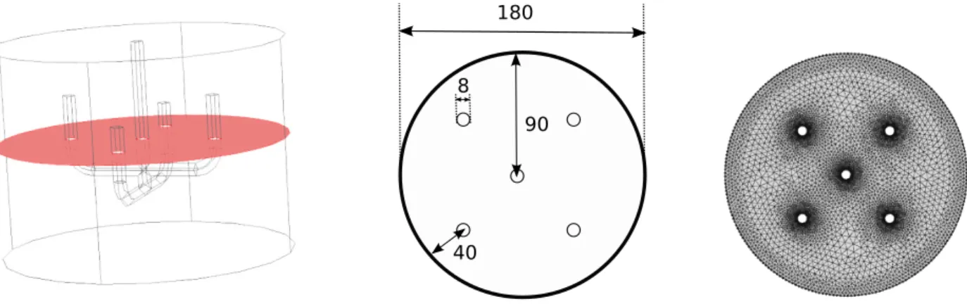
In this study, synthetic data were generated to test the parameter identification methodology described in Section 2. In order to consider realistic conditions, the synthetic data came from the simulation of a non-conventional shearing geometry (Figure 2, [41]) that minimized the heterogeneity of cement-based suspensions during the rheometric test (see Section 1).

180

3.1. CFD Simulation

The CFD simulation was performed with the COMSOL Multiphysics finite element software [42]. To save computational time, a 2D model (Figure 2) was preferred over a 3D model. This simplification did not affect the identification procedure, as the input was synthetic data. Preliminary results showed that such a simplification would not be worth considering for real experimental data.

COMSOL 5.0.0.244

40

90 180 8

Figure 2: 3D diagrammatic representation of the anchor impeller (left), horizontal cross section of the shearing geometry (cylindrical tank and anchor impeller) with dimensions in millimeters (middle), and optimized finite element mesh with 11742 triangular elements and with second order elements for velocity and first order elements for pressure (right).

Studies show that a three-parameter behavior law is necessary for a good description of cement-based materials. In particular, the Herschel-Bulkley model described in Eq. (3) is suitable for fitting the cement-based material data [10, 29, 30, 43, 44].

τ = τ0+ K ˙γn, (3)

where τ is the shear stress, ˙γ the shear rate, τ0 the yield stress, n the behavior index and K the consistency

index.

τ0is the offset of the curve (due to cohesion strength) and n gives the material the shear-thickening property

if n > 1 or shear-thinning if n < 1. For n = 1 Eq. (3) matches the Bingham model. The fundamental meaning of Herschel-Bulkley fluid implies an infinite viscosity when the shear rate approaches zero. To avoid this calculation issue, regularization methods have been developed [45–47]. The method adopted in this study

is presented in Eq. (4). ˙γc was set to 10−1s−1 following a preliminary sensitivity study. Figure 3 shows the

apparent viscosity as a function of the shear rate, as given by the original and regularized versions. η( ˙γ) =τ0 ˙ γ + K ˙γ (n−1) _{for ˙γ ≥ ˙γ} c η( ˙γ) = τ0 ˙ γc+ K ˙γ (n−1) c for ˙γ ≤ ˙γc (4)

In this study, the flow was considered as steady, laminar, incompressible, isothermal and homogeneous.

190

The differential equations for mass conservation and momentum balance were directly implemented in the finite-element software (Eq. (5) and (6)).

ρ∂ ~V

∂t + ρ~V · grad~V = − ~gradp + ~divτ + ρ~g (5)

γ˙c µ γ˙ Regularized viscosity γ˙c µ γ˙ Regularized viscosity Original viscosity γ˙c µ γ˙

Figure 3: Herschel-Bulkley and chosen regularized viscosities.

where ~V is the speed vector, ρ the density, p the pressure, τ the Cauchy stress tensor and ~g the gravity

vector.

To simplify the boundary conditions of the finite-element model, computations were conducted in a rotating

195

frame bound to the impeller. The motion of this frame required the introduction of centrifugal and Coriolis forces to the momentum balance (Eq. (5)) [48]. Based on a preliminary study showing that the results did not depend on the mesh, the FE model contained 11742 triangular elements: second order elements were used for velocity and first order elements for pressure (Figure 2).

3.2. Identification for Herschel-Bulkley model

200

3.2.1. Parameter search space

The parameter search space, defined in Table 1, corresponded to classical values for cement-based sus-pensions [49]. Selected optimization algorithms required parameter grid inputs. The step for each parameter was set according to a previous sensitivity study.

Minimal value Maximal value Step Triplet 1 Triplet 2

τ0 [P a] 0 50 5 20 45

K [P a.sn_{] 5 50 5 30 45}

n 0.5 1.2 0.05 1.1 0.6

Table 1: Parameter search space and solution triplets tested

Since the reference data were generated numerically, the solution parameters were known a priori and

205

selected in the parameter search space. In order to represent the diversity of shapes of the objective function and thus to test the identification methodology in different conditions, two solution parameter triplets were selected in two different areas of the parameter search space. The first triplet presented a shear-thickening behavior (n = 1.1) and the second a shear-thinning behavior (n = 0.6). With the intention of considering suspensions currently used in the concrete industry, two representative yield stresses of Self Compacting

210

index was determined by analogy with Bingham plastic viscosity values ranging from 25 [P a.s] to 35 [P a.s]

and typical shear rate values corresponding to concrete pouring (see, e.g., [52]), so that the (τ0,K,n) triplets

reflected an acceptable SCC according to the validity diagram defined by Wallevik [50]. The final triplets are summarized in Table 1. Although both combinations of Herschel-Bulkley parameters defined in Table 1 lead

215

to the self-compacting ability of concrete, it is important to specify that the literature highlights behavior index values always greater than one for SCC, both at the experimental [41] and the local [53] levels. However this fact does not invalidate the shear-thinning triplet, as the aim of this paper was to determine the efficiency of the optimization algorithms, which depends directly on the shape of the objective function, from synthetic data. Considering real data would modify the shape of the function without the user knowing, a priori, the

220

shape of the function.

3.2.2. Identification procedures

According to the user’s knowledge of the rheological behavior of the material under study, different, more or less complex, identification procedures can be performed. In this study, three different levels of knowledge of the material, defined as approaches, were considered. For each approach, two or three procedures were

225

studied (Figure 4).

Macroscopic curve

T vs ω (τ0,K,n)

Approach 1 : No a priori knowledge is supposed

(τ₀,K,n) Genetic algorithm

Simplex

Macroscopic curve

T vs ω (τ0,K,n)

Approach 2: A conservation of behavior in both the experimental and the local planes is supposed

(τ₀,K,n) Genetic algorithm

Simplex

Macroscopic curve

T vs ω n=m (τ0,K)

Approach 3: Empirical relationship between the parameters of experimental curve and those of local curve

Initialization

(τ₀,K) (τ0,K)

Logarithmic transposition Genetic algorithm

Simplex Empirical relationships Least-squares method Initialization (τ₀,K) (τ0,K) Simplex Random 1_GA 1_S 2_GA 2_S 3_GA 3_S 3_init_S Shear-thinning / Shear-thickening Macroscopic curvature

Figure 4: Identification procedures according to the user’s knowledge about the material.

In the first approach, the user is supposed to know nothing about the behavior of the studied material a priori. For Procedure 1 GA (resp. Procedure 1 S) optimization was carried out by means of a genetic algorithm (resp. the simplex algorithm). The 3D parameter search space needed to be wide enough to

include the material parameters.

230

In a second approach, the user is supposed to know whether the studied material is shear-thickening or shear-thinning. For materials whose nature is clearly established, this approach is particularly appropriate. It allows the user to reduce the parameter search space (n ≥ 1 or n ≤ 1), which speeds up the optimization

process. As previously mentioned for Approach 1, optimization was carried out by means of a genetic

algorithm and the simplex algorithm.

235

Finally, in the third approach, the user is supposed to know a priori correlations between the parameters in the ( ˙γ,τ )-plane and the (ω,T )-plane, as proposed in [19]. In order to estimate the influence of such information, the following relation was assumed because it was already used for cement-based suspensions [54].

T = T0+ kωm (7)

where T0, k and m are constants.

240

Under this assumption, preliminary studies have highlighted the following correlations:

n [∅] ≈ m (8)

τ0[P a] ≈ 1200 × T0[N.m] (9)

K [P a.sn] kh_rpmN.mm

i ≈ 1200exp(1.8m) (10)

Note that the use of these correlations is limited to this specific study, i.e. this parameter search space, Herschel-Bulkley model, geometry and boundary conditions. The first correlation has already been suggested in the literature [7]. It allows for a two-parameter identification and therefore a restriction of the parameter search space to two dimensions. The value of m can be determined by a logarithmic transposition of Eq. (7).

245

Procedure 3 GA was based on a genetic optimization whereas Procedure 3 S and Procedure 3 init S were based on the simplex method. The differences between the two latter methods lie in the initialization of the simplex, as explained in Section 4.3.

3.2.3. Algorithm parameters

For both algorithms, the optimization procedure was performed by modeFRONTIER [55]. In this study,

250

the number of individuals in the initial population varied only with the dimensions of the search space, so that the influence of the objective function could be discussed. The selected values are presented in Table 2 and are in agreement with the range given in [40]. Note that the modeFRONTIER user manual [55] recommends defining an initial population with more than 16 individuals. These populations were randomly generated with a uniform distribution, which increases the robustness and avoids premature convergence [56].

255

The size of the population was kept constant during the optimization process. The probability of directional cross-over was set to 0.5, the probability of selection to 0.05 and the probability of mutation to 0.1. These

values follow the recommendations of the user manual [55] and are similar to those given in the literature [57]. Optimization was considered as completed after five generations.

Nb of sets in the search space Nb of individuals in the population

Approach 1 1650 100

Approach 2 shear-thickening 550 35

Approach 2 shear-thinning 1210 75

Approach 3 110 16

Table 2: Number of individuals in the population for the MOGA-II method

As previously mentioned, the results given by the simplex method may depend on the initialization.

260

That is why, in this study, each identification procedure based on the simplex method was performed three

times. The tolerance value for the stopping criterion was set to 10−3_{. For two-parameter identification, the}

simplex consisted of three vertices and for three-parameter identification, it consisted of four vertices. For Procedure 1 S, Procedure 2 S and Procedure 3 S, the initial simplex was randomly generated with a uniform distribution. For Procedure 3 init S, the correlations (8), (9) and (10) were used to initialize the simplex.

265

4. Identification results and discussion

In this section, the identification results obtained considering successively the three approaches described in Section 3 are presented, discussed and compared. The shear-thinning and shear-thickening materials are examined for each procedure.

4.1. Approach 1: no a priori knowledge about the material behavior

270

Procedure 1 S was carried out first. Table 3 summarizes the initial simplexes and the optimal sets of parameters obtained with this procedure for the shear-thickening material. None of these calculations led to the mathematical solution. From a physical point of view, satisfactory sets of parameters could be defined as the sets of parameters for which the value of the objective function was lower than a value corresponding to

the scattering error associated with the experimental device. In this study, this value was set to 5.44 × 10−4

275

[(N.m)2] (resp. to 2.50×10−4[(N.m)2]) for the shear-thickening (resp. shear-thinning) material. Considering

this criterion, two optimal sets of parameters were satisfactory. Figure 5 highlights the difference between the solution set and a satisfactory set of parameters in terms of (ω,T ) and ( ˙γ,τ ) curves.

The three optimal sets of parameters presented the same values of the behavior index (n = 1.1) and the

consistency index (K = 30 [P a.sn_{]) as the solution set and different values for the yield stress. This may}

280

point out great sensitivity to the behavior and consistency indexes and slight sensitivity of the rheometric curve to the yield stress. From a mathematical point of view, this is expressed as a sloping objective function regarding the variables n and K in the vicinity of the solution and a flat objective function regarding the

0 0.1 0.2 0.3 0.4 0.5 0.6 0.7 0 20 40 60 80 100

T

ω

τ

γ

˙

Figure 5: (ω, T ) and ( ˙γ,τ ) curves corresponding to the reference triplet (20,30,1.1) and to the satisfactory triplet (0,40,1) with Fobj= 4.4641 × 10−4[(N.m)2].

variable τ0. Moreover, despite the initial sets of parameters being distributed over the whole search space,

the optimal sets of parameters were located in the vicinity of the solution. This may indicate a pronounced

285

global minimum of the objective function.

Initial sets Optimal set

τ0[P a],K[P a.sn],n[∅] Fobj [(N.m)2] τ0[P a],K[P a.sn],n[∅] Fobj [(N.m)2] nb of evaluations

(30,40,0.5) 5.2501 × 10−1 (5,30,1.1) 2.3048 × 10−3 29 (0,15,1.05) 4.0462 × 10−1 (35,25,0.75) 4.1886 × 10−1 (45,10,0.85) 6.2948 × 10−1 (15,40,1.15) 2.2684 × 10−1 (15,30,1.1) 2.5552 × 10−4 21 (10,35,0.75) 3.2026 × 10−1 (5,40,0.45) 6.6665 × 10−1 (25,45,0.45) 5.4948 × 10−1 (30,35,1.15) 1.3210 × 10−1 (25,30,1.1) 2.5532 × 10−4 35 (0,30,0.8) 2.1620 × 10−1 (30,50,1) 1.1572 × 10−1 (10,15,0.9) 5.6543 × 10−1

Table 3: Results obtained with Procedure 1 S for the triplet (20,30,1.1)

The same procedure was applied to the shear-thinning material (45,45,0.6). The results are presented in Table 4. The exact solution was obtained once out of the three calculations. The other optimal sets could not be considered as satisfactory. In particular, the first optimization run led to an optimal set for which the objective function value was ten times higher than for the other optimal sets with a reduced number of

evaluations. This premature convergence might result from the existence of a valley in the objective function (Table 4), as mentioned by [31].

Initial sets Optimal set

τ0[P a],K [P a.sn],n [∅] Fobj [(N.m)2] τ0[P a],K [P a.sn],n [∅] Fobj [(N.m)2] nb of evaluations

(30,35,1.15) 8.3290 × 10−1 (0,40,0.65) 1.5701 × 10−2 11 (0,30,0.9) 1.1612 × 10−2 (30,50,1) 7.7722 × 10−1 (10,15,0.9) 5.5481 × 10−1 (30,40,0.6) 8.0579 × 10−2 (45,45,0.6) 0 33 (0,15,1.1) 2.1082 × 10−1 (35,25,0.8) 5.3136 × 10−3 (45,10,0.8) 5.4274 × 10−2 (45,40,0.9) 1.6672 × 10−1 (40,30,0.75) 1.4210 × 10−3 21 (45,15,0.45) 1.1315 × 10−1 (25,15,0.75) 8.0465 × 10−2 (50,5,0.5) 1.7831 × 10−1

Table 4: Results obtained with Procedure 1 S for the triplet (45,45,0.6)

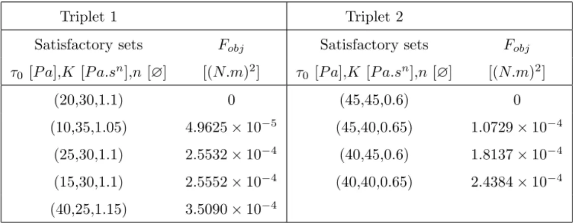
Procedure 1 GA was carried out successively for the shear-thickening and shear-thinning materials. It involved a population of 100 individuals, initially randomly distributed over the 1650 triplets of the search space. For both materials, the solution triplet emerged and some other satisfactory triplets were detected

295

(Table 5). For both materials, the individuals whose parameter n is equal to the solution value represent more than a quater of the last population. This shows the large sensitivity to this parameter.

Triplet 1 Triplet 2

Satisfactory sets Fobj Satisfactory sets Fobj

τ0[P a],K [P a.sn],n [∅] [(N.m)2] τ0 [P a],K [P a.sn],n [∅] [(N.m)2]

(20,30,1.1) 0 (45,45,0.6) 0

(10,35,1.05) 4.9625 × 10−5 (45,40,0.65) 1.0729 × 10−4

(25,30,1.1) 2.5532 × 10−4 (40,45,0.6) 1.8137 × 10−4

(15,30,1.1) 2.5552 × 10−4 (40,40,0.65) 2.4384 × 10−4

(40,25,1.15) 3.5090 × 10−4

Table 5: Satisfactory sets for Procedure 1 GA

In order to make the computational cost independent of the performance of the computer, the elementary simulation of a rheometric test was considered as the unit of measurement. The simplex method led to 85

simulations for the shear-thickening material and to 65 simulations for the shear-thinning one. The genetic

300

algorithm was stopped after 500 simulations. It is clear that the computational cost with the genetic method was higher. However, this method led not only to the exact solution but also to a set of satisfactory parameters and to reliable information about the sensitivity to the parameters. The simplex method rapidly provided an optimal set, which could be unsatisfactory.

To go further into the comparison between the simplex and genetic methods, the objective functions

305

corresponding to the shear-thickening and shear-thinning materials were computed on the entire parameter search space. Figure 6 (resp. 7) represents the normalized objective function values, i.e. objective function

values divided by 5.44 × 10−4 [(N.m)2_{] (resp. 2.50 × 10}−4 _[(N.m)2_{]), as a function of the three constitutive}

parameters for the shear-thickening (resp. shear-thinning) material. The high sensitivity of the objective function regarding the parameters n and K was noticeable on both figures.

310 5 10 15 20 25 30 35 40 45 _{50 0} 10 20 30 40 50 0.6 0.8 1 1.2

n

K

τ

n

F

Figure 6: Normalized objective function values smaller than 14 for the triplet (20,30,1.1).

5 10 15 20 25 30 35 40 45 _{50 0} 10 20 30 40 50 0.6 0.8 1 1.2

n

K

τ

n

F

4.2. Approach 2: the material is shear-thinning or shear-thickening

In this section, the shear-thickening or shear-thinning property of the material is considered to be known and this behavior is assumed to be observed in the macroscopic state ((ω,T )-plane) as well as in the local state (( ˙γ,τ )-plane). These assumptions allow the user to restrict the parameter search space.

For the shear-thickening material, n was sought in the range [1, 1.2]. To test Procedure 2 S, four initial

315

triplets were randomly chosen in the reduced search space. As shown in Table 6, the exact solution was detected once and the other two optimal sets were satisfactory. The efficiency of the simplex method was enhanced with the use of this procedure.

Initial sets Optimal set

τ0 [P a],K [P a.sn],n [∅] Fobj [(N.m)2] τ0 [P a],K [P a.sn],n [∅] Fobj [(N.m)2] nb of evaluations

(30,40,1) 6.6996 × 10−3 (20,30,1.1) 0 25 (0,15,1.2) 1.8472 × 10−1 (35,25,1.1) 1.7730 × 10−2 (45,10,1.1) 3.8894 × 10−1 (15,35,1.2) 2.5763 × 10−1 (40,25,1.15) 3.0509 × 10−4 29 (20,35,1.15) 1.1275 × 10−1 (45,5,1.1) 6.3582 × 10−1 (45,40,1.1) 1.7446 × 10−1 (30,35,1) 2.2831 × 10−1 (25,30,1.1) 2.5532 × 10−4 17 (35,30,1.15) 5.3406 × 10−1 (40,25,1.2) 4.6559 × 10−1 (25,10,1.1) 2.9193 × 10−2

Table 6: Results obtained with Procedure 2 S for the triplet (20,30,1.1)

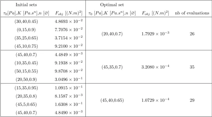
For the shear-thinning material, the range of the possible values of n was restricted to [0.5, 1]. The exact solution was never reached and only one optimal set could be considered as a satisfactory set (Table 7).

320

For this material, the restriction of the search space did not enhance the efficiency of the method as the restriction concerned only the n-axis and did not prevent the algorithm from getting stuck in the plateau of

the objective function along the τ0- and K-axes (see Figure 7 and Section 4.1).

Table 8 summarizes the satisfactory sets obtained with the genetic method. For the shear-thinning

material, more satisfactory sets were detected with Procedure 2 GA than with Procedure 1 GA, which

325

indicates that the efficiency of the genetic method was enhanced. For the shear-thickening material, only three satisfactory sets were detected. This can be explained by the small number of individuals in the population, which could have led to premature convergence.

Initial sets Optimal set

τ0[P a],K [P a.sn],n [∅] Fobj [(N.m)2] τ0[P a],K [P a.sn],n [∅] Fobj [(N.m)2] nb of evaluations

(30,40,0.45) 4.8693 × 10−2 (20,40,0.7) 1.7929 × 10−3 26 (0,15,0.9) 7.7076 × 10−2 (35,25,0.65) 3.7154 × 10−2 (45,10,0.75) 9.2100 × 10−2 (45,40,0.7) 4.4849 × 10−3 (45,35,0.7) 3.2080 × 10−4 35 (10,35,0.45) 9.1938 × 10−2 (50,15,0.55) 9.8708 × 10−2 (20,50,0.9) 3.0496 × 10−1 (15,35,0.95) 1.0915 × 10−1 (45,40,0.65) 1.0729 × 10−4 ₂₉ (20,35,0.8) 8.1587 × 10−3 (45,5,0.65) 1.6308 × 10−1 (45,40,0.7) 4.8490 × 10−3

Table 7: Results obtained with Procedure 2 S for the triplet (45,45,0.6)

Triplet 1 Triplet 2

Satisfactory sets Fobj Satisfactory sets Fobj

τ0[P a],K [P a.sn],n [∅] [(N.m)2] τ0 [P a],K [P a.sn],n [∅] [(N.m)2]

(15,30,1.1) 2.5552 × 10−4 (45,45,0.6) 0 (40,25,1.15) 3.5090 × 10−4 (45,40,0.65) 1.0729 × 10−4 (35,25,1.15) 3.5984 × 10−4 (50,50,0.55) 1.7330 × 10−4 (50,45,0.6) 1.8052 × 10−4 (40,45,0.6) 1.8137 × 10−4 (40,40,0.65) 2.4384 × 10−4

Table 8: Satisfactory sets for Procedure 2 GA

4.3. Approach 3: the behavior index is known

In this part, the relation n = m is assumed and the parameter search space is confined to two parameters:

330

τ0 and K. The results obtained with Procedure 3 S for the thickening triplet are summarized in Table 9.

The simplex method provided the exact solution two times out of three. The third time, the optimal set was unsatisfactory. This resulted from a premature convergence, probably due to a misshaped initial simplex. For the shear-thinning material, the exact solution was not reached but, two times out of three, the solutions were satisfactory (Table 10). As long as the initial simplex was well-shaped, the reduction of parameters to

335

Initial sets Optimal set

τ0 [P a],K [P a.sn],n [∅] Fobj [(N.m)2] τ0 [P a],K [P a.sn],n [∅] Fobj [(N.m)2] nb of evaluations

(20,35,1.1) 2.9939 × 10−2 (20,25,1.1) 2.9928 × 10−2 8 (15,10,1.1) 4.9775 × 10−1 (10,10,1.1) 5.1775 × 10−1 (5,40,1.1) 9.3009 × 10−2 (20,30,1.1) 0 17 (5,20,1.1) 1.5095 × 10−1 (20,20,1.1) 1.1968 × 10−1 (40,40,1.1) 1.6251 × 10−1 (20,30,1.1) 0 29 (15,5,1.1) 7.7708 × 10−1 (45,10,1.1) 3.8894 × 10−1

Table 9: Results obtained with Procedure 3 S for the triplet (20,30,1.1)

Initial sets Optimal set

τ0[P a],K [P a.sn],n [∅] Fobj [(N.m)2] τ0[P a],K [P a.sn],n[∅] Fobj [(N.m)2] nb of evaluations

(30,40,0.6) 8.0579 × 10−3 (50,45,0.6) 1.8052 × 10−4 11 (10,10,0.6) 1.9959 × 10−1 (45,5,0.6) 1.1715 × 10−1 (25,35,0.6) 2.3403 × 10−2 (35,45,0.6) 7.2991 × 10−4 9 (35,50,0.6) 6.7544 × 10−4 (15,25,0.6) 7.8102 × 10−2 (0,40,0.6) 2.9614 × 10−2 (50,45,0.6) 1.8052 × 10−4 14 (25,5,0.6) 2.0941 × 10−1 (45,35,0.6) 1.1019 × 10−2

Table 10: Result obtained with Procedure 3 S for the triplet (45,45,0.6)

The genetic algorithm was used with a population of 16 individuals as described in Procedure 3 GA. For both behaviors, the reduction in the number of parameters to be identified led to a diminution of the number of satisfactory individuals in the search space and therefore to a limitation of the non-uniqueness of the problem solution. For the shear-thickening material, all satisfactory parameter sets were detected,

340

whereas, for the shear-thinning triplet, two satisfactory sets out of three were determined (Table 11). The difference observed between the results with the simplex and the genetic methods was confirmed by Figure 8 representing the isovalues of the normalized objective function for n = 1.1 and for n = 0.6. In the

vicinity of the solution, the gradient with respect to τ0 was smaller than the gradients with respect to K for

both cases. Whereas, for the shear-thickening case, the isovalues were situated like Russian nesting dolls, the

Triplet 1 Triplet 2

Satisfactory sets Fobj Satisfactory sets Fobj

τ0[P a],K [P a.sn],n [∅] [(N.m)2] τ0 [P a],K [P a.sn],n [∅] [(N.m)2]

(20,30,1.1) 0 (45,45,0.6) 0

(25,30,1.1) 2.5532 × 10−4 (40,45,0.6) 1.8137 × 10−4

(15,30,1.1) 2.5552 × 10−4

Table 11: Satisfactory sets for Procedure 3 GA

objective function of the shear-thinning case presented a plateau - which did not coincide with the smallest isovalue (given the input grid). This explains the difficulties encountered by the algorithms for shear-thinning behavior. 10 15 20 25 30 35 40 45 50 20 25 30 35 40 45 50 τ 0 [Pa] K [Pa.s1.1] Satisfactory triplets 0 100 200 300 400 500 600 700 800 900 F_obj norm 10 15 20 25 30 35 40 45 50 20 25 30 35 40 45 50 τ 0 [Pa] K [Pa.s0,6] Satisfactory triplets 0 50 100 150 200 250 300 350 F_obj norm

Figure 8: Contours of the objective function for the triplet (20,30,1.1) (left) and for the triplet (45,45,0.6) (right).

Assuming that empirical relations exist between the parameters in the ( ˙γ,τ )-plane and the (ω,T )-plane, they could be used to determine the initial simplex (Procedure 3 init S). Relations 9 and 10 correspond to

350

an average tendency and were used to define the initial triplets (Table 12). For both materials, the exact triplet was detected after 16 (resp. 8) iterations for the shear-thickening (resp. shear-thinning) material.

Triplet 1 Triplet 2

τ0[P a],K [P a.sn],n [∅] Fobj [(N.m)2] τ0 [P a],K [P a.sn],n [∅] Fobj [(N.m)2]

(25,30,1.1) 2.5532 × 10−2 (35,35,0.6) 1.6045 × 10−2

(20,20,1.1) 1.1968 × 10−1 _{(30,40,0.6) 8.0579 × 10}−3

(35,30,1.1) 4.0626 × 10−2 (45,45,0.6) 0

4.4. Comparison among the three approaches

The results given by the three approaches are summarized in Table 13. According to the identification results presented in Section 4.1 and the shape of the objective functions, it seems that, for a three-parameter

355

identification, the simplex method would be good enough for the shear-thickening material (two out of three optimal sets were satisfactory), whereas the genetic method would be necessary for the shear-thinning material. As shown in Section 4.2, the restriction of the parameter range particularly benefited the simplex method based on a local search for the solution. However, this restriction did not modify the objective function in the vicinity of the solution. That is why the identification of the shear-thinning material with

360

the simplex method was not improved and the genetic method appeared to be more reliable. Finally, for a two-parameter identification, the shape of the objective function was modified and both the simplex method and the genetic method were reliable. However, given the computational cost, the simplex method seemed to be the more efficient. As previously mentioned, the user does not have a priori knowledge of the shape of the objective function. Therefore the authors recommend using the genetic method for a three-parameter

365

identification and the simplex method for a two-parameter identification.

Simplex method Genetic method Genetic method

Nsatisfactory sets/ Ndetected satisfactory sets/ Ndetected satisfactory sets/

Noptimizations Nsatisfactory sets Npopulation individuals

Approach 1 n = 1.1 2/3 5/10 5/100 n = 0.6 1/3 4/7 4/100 Approach 2 n = 1.1 3/3 3/10 3/35 n = 0.6 1/3 6/7 6/75 Approach 3 n = 1.1 2/3 3/3 3/16 n = 0.6 2/3 2/3 2/16 Approach 3 n = 1.1 1/1 (empirical relations) n = 0.6 1/1

Table 13: Synopsis of the results obtained with the three approaches

5. Conclusions and prospects

In this study, inverse analysis was applied to two specific cement-based suspensions (one shear-thinning and the other shear-thickening) using rheometric data obtained with a specific impeller. As it was a first step of a larger study, the application was limited to synthetic data. The efficiency of two kinds of algorithms

370

(stochastic and deterministic) was compared by taking account of the user’s a priori knowledge about the value of the parameters to be identified. In this study, an algorithm was considered as effective when one or more satisfactory sets were systematically detected in a short computational time. For both materials,

the genetic method appeared to be suitable for the identification of three parameters over a large search space, whereas the simplex method allowed effective parameter identification when two parameters had to

375

be identified and when the initial simplex was well-shaped. Both algorithms encountered more difficulties with the shear-thinning material than with the shear-thickening one. This was confirmed by the shape of the objective function.

This study corresponds to a first step in the procedure for identifying rheological parameters of

cement-380

based suspensions. A second step will consist in using real experimental data. This will (surely) lead to noisy objective functions. Under these conditions, the genetic method might be more suitable, even for a two-parameter identification. Moreover, inverse analysis assumes that the constitutive relation can reproduce the material behavior perfectly, which is not realistic. Therefore the objective function is expected to be more complex. Finally it has been mentioned several times in this paper that, in the context of the study, the

385

sensitivity to the yield stress τ0 was lower than that to the consistency and the behavior indexes. That

is why the satisfactory sets included sets with different τ0-values. One may wonder which satisfactory set

it is best to select, considering the possible consequences on the prediction of the material flow in different contexts. Actually, additional experimental data, obtained with a different experimental device with enhanced sensitivity to the yield stress, are necessary and would serve for disambiguation purposes. In that way,

390

obtaining several satisfactory sets as provided by the genetic method would give more reliable identification insofar as the user can contribute his scientific expertise and/or has additional experimental data at his disposal, obtained by other means than the use of a rheometer.

References

[1] H. A. Barnes, J. F. Hutton, K. Walters, An introduction to rheology, Elsevier, 1989.

395

[2] A. Iranshahi, M. Heniche, F. Bertrand, P. A. Tanguy, Numerical investigation of the mixing efficiency of the Ekato Paravisc impeller, Chemical Engineering Science 61 (2006) 2609–2617.

[3] D. Anne-Archard, H. C. Marouche, M. Boisson, Hydrodynamics and Metzner-Otto correlation in stirred vessels for yield stress fluids, Chemical Engineering Journal 125 (2006) 15–24.

[4] P. Prajapati, F. Ein-Mozaffari, CFD investigation of the mixing of yield-pseudoplastic fluids with anchor

400

impellers, Chemical Engineering & Technology 32 (2009) 1211–1218.

[5] D. O. Olukanni, J. J. Ducoste, Optimization of waste stabilization pond design for developing nations using computational fluid dynamics, Ecological Engineering 37 (11) (2011) 1878–1888.

[6] L. Pakzad, F. Ein-Mozaffari, S. R. Upreti, A. Lohi, Agitation of Herschel-Bulkley fluids with the Scaba-anchor coaxial mixers, Chemical Engineering Research and Design 91 (2013) 761–777.

[7] G. Heirman, L. Vandewalle, D. Van Gemert, O. Wallevik, Integration approach of the Couette inverse problem of powder type self compacting concrete in a wide-gap concentric cylinder rheometer, Journal of Non-Newtonian Fluid Mechanics 150 (2008) 93–103.

[8] R. M. Turian, T. W. Ma, F. L. G. Hsu, D. J. Sung, Characterization, settling, and rheology of concen-trated fine particulate mineral slurries, Powder Technology 93 (3) (1997) 219–233.

410

[9] T. Hemphill, W. Campos, A. Pilehvari, Yield-power law model more accurately predicts mud rheology, Oil and Gas Journal 91 (34) (1993) 45–50.

[10] A. Papo, Rheological models for cement pastes, Materials and Structures 21 (1988) 41–46.

[11] S. Khataniar, G. A. Chukwu, H. Xu, Evaluation of rheological models and application to flow regime determination, Journal of Petroleum Science and Engineering 11 (1994) 155–164.

415

[12] W. J. Bailey, I. S. Weir, Investigation of methods for direct rheological model parameter estimation, Journal of Petroleum Science and Engineering 21 (1998) 1–13.

[13] C. Legrand, Contribution to the study of the fresh concrete rheology - in French, Mat´eriaux et

Con-struction 5 (5) (1972) 275–295.

[14] M. R. Geiker, M. Brandl, L. N. Thrane, D. H. Bager, O. Wallevik, The effect of measuring procedure

420

on the apparent rheological properties of self-compacting concrete, Cement and Concrete Research 32 (2002) 1791–1795.

[15] J. Bhatty, P. Banfill, Sedimentation behaviour in cement pastes subjected to continuous shear in rota-tional viscometers, Cement and Concrete Research 12 (1) (1982) 69–78.

[16] W. Yao, M. Mishima, K. Takahashi, Numerical investigation on dispersive mixing characteristics of

425

MAXBLEND and double helical ribbons, Chemical Engineering Journal 84 (3) (2001) 565–571. [17] M. Zhang, L. Zhang, B. Jiang, Y. Yin, X. Li, Calculation of Metzner constant for double helical ribbon

impeller by computational fluid dynamic method, Chinese Journal of Chemical Engineering 16 (2008) 686–692.

[18] M. Ohta, M. Kuriyama, K. Arai, S. Saito, A two-dimensional model for the secondary flow in an agitated

430

vessel with anchor impeller, Journal of Chemical Engineering of Japan 18 (1985) 81–84.

[19] O. H. Wallevik, D. Feys, J. E. Wallevik, K. H. Khayat, Avoiding inaccurate interpretations of rheological mesurements for cement-based materials, Cement and Concrete Research 78 (2015) 100–109.

[20] A. B. Metzner, R. E. Otto, Agitation of non-Newtonian fluids, American Institute of Chemical Engineers Journal 3 (1) (1957) 3–10.

[21] G. Delaplace, J. C. Leuliet, V. Relandeau, Circulation and mixing times for helical ribbon impellers. Review and experiments, Experiments in fluids 28 (2) (2000) 170–182.

[22] M. Bousmina, A. Ait-Kadi, J. B. Faisant, Determination of shear rate and viscosity from batch mixer data, Journal of Rheology 43 (2) (1999) 415–433.

[23] H. Roos, U. Bolmstedt, A. Axelsson, Evaluation of new methods and measuring systems for

characteri-440

sation of flow behaviour of complex foods, Applied Rheology 10 (2006) 19–25.

[24] P. Estell´e, C. Lanos, Shear flow curve in mixing systems- A simplified approach, Chemical Engineering

Science 154 (2008) 31–38.

[25] A. Nzihou, B. Bournonville, P. Marchal, L. Choplin, Rheology and heat transfer during mineral residue phosphatation in a rheo-reactor, Chemical Engineering Research and Design 82 (2004) 637–641.

445

[26] P. F. G. Banfill, D. S. Swift, The effect of mixing on the rheology of cement-based materials containing high performance superplasticisers, Annual transactions of the Nordic Rheology Society 12 (2004) 9–12. [27] H. S. Tang, D. M. Kalyon, Estimation of the parameters of Herschel-Bulkley fluid under wall slip using

a combination of capillary and squeeze flow viscometers, Rheological Acta 43 (2008) 80–88. [28] M. Al-Chalabi, When least-squares squares least, Geophysical Prospecting 40 (1992) 359–378.

450

[29] M. Nehdi, M. A. Rahman, Estimating rheological properties of cement pastes using various rheological models for different test geometry, gap and surface friction, Cement and Concrete Research 34 (2004) 1993–2007.

[30] A. Yahia, K. H. Khayat, Applicability of rheological models to high-performance grouts containing supplementary cementitious materials and viscosity enhancing admixture, Materials and Structures 36

455

(2003) 402–412.

[31] J. A. Nelder, R. Mead, A method for function minimization, The Computer Journal 7 (1965) 308–313. [32] V. C. Kelessidis, R. Maglione, C. Tsamantaki, Y. Aspirtakis, Optimal determination of rheological parameters for Herschel-Bulkley drilling fluids and impact on pressure drop, velocity profiles and pene-tration rates during drilling, Journal of Petroleum Science and Engineering 53 (2006) 203–224.

460

[33] C. F. Ferraris, F. de Larrard, Testing and modelling of fresh concrete rheology, National Institute of Standards and Technology, Gaithersburg, USA, 1998.

[34] J. H. Holland, Adaptation in natural and artificial systems: An introduction analysis with application to biology, control and artificial intelligence, University of Michigan Press, Ann Arbor, MI, 1975. [35] D. E. Goldberg, J. H. Holland, Genetic algorithms and machine learning, Machine Learning 3 (2) (1988)

465

[36] D. Bhandari, C. A. Murthy, S. K. Pal, Variance as a stopping criterion for genetic algorithms with elitist model, Fundamenta Informaticae 120 (2012) 145–164.

[37] C. Poloni, V. Pediroda, GA coupled with computationally expensive simulations: tools to improve

efficiency, in: D. Quagliarella, J. P´eriaux, C. Poloni, G. Winter (Eds.), Genetic algorithms and evolution

470

strategies in engineering and computer science, Wiley, West Sussex, England, 267–288, 1997. [38] S. Poles, MOGA-II An improved Multi-Objective Genetic Algorithm, Tech. Rep., Esteco, 2003. [39] S. Poles, E. Rigoni, T. Robic, MOGA-II performance on noisy optimization problems, in: B. Filipic,

J. Silc (Eds.), International Conference on Bioinspired Optimization Methods and their Applications, Jozef Stefan Institute, Ljubljana, Slovenia, 51–62, 2004.

475

[40] K. F. Man, K. S. Tang, S. Kwong, Genetic algorithms: concepts and applications, IEEE Transactions on Industrial Electronics 43 (5) (1996) 519–534.

[41] M. Mouret, M. Cyr, A discussion of the paper ”The effect of measuring procedure on the apparent rheological properties of self-compacting concrete” by M. R. Geiker et al., Cement and Concrete Research 33 (11) (2003) 1901–1903.

480

[42] COMSOL, COMSOL multiphysics user guide (Version 4.4), COMSOL, 2013.

[43] A. Yahia, K. H. Khayat, Analytical models for estimating yield stress of high-performance pseudoplastic grout, Cement and Concrete Research 31 (2001) 731–738.

[44] C. Atzeni, L. Massidda, U. Sanna, Comparison between rheological models for portland cement pastes, Cement and Concrete Research 15 (1985) 511–519.

485

[45] M. Bercovier, M. Engelman, A finite-element method for incompressible non-Newtonian flows, Journal of Computational Physics 36 (3) (1980) 313–326.

[46] T. C. Papanastasiou, Flows of materials with yield, Journal of Rheology 31 (5) (1987) 385–404. [47] R. I. Tanner, J. F. Milthorpe, Numerical simulation of the flow of fluids with yield stress, in: C. Taylor,

J. A. Johnson, W. R. Smith (Eds.), Numerical methods in laminar and turbulent flow, Pineridge Press,

490

680–690, 1983.

[48] M. Marouche, D. Anne-Archard, H. C. Boisson, A numerical model of yield stress fluid dynamics in a mixing vessel, Applied Rheology 12 (4) (2002) 182–191.

[49] M. Cyr, Contribution to the characterization of mineral admixtures and the understanding of their actions on the rheological behavior of the cementitious materials - in French, Ph.D. thesis, INSA

495

[50] O. H. Wallevik, Rheology–a scientific approach to develop self-compacting concrete, in: O. Wallevik, I. Nielsson (Eds.), International RILEM Symposium on Self-Compacting Concrete, RILEM Publications SARL, 23–31, 2003.

[51] N. Roussel, P. Coussot, Fifty-cent rheometer for yield stress measurements: from slump to spreading

500

flow, Journal of Rheology 49 (3) (2005) 705–718.

[52] C. Artelt, E. Garcia, Impact of superplasticizer concentration and of ultra-fine particles on the rheological behaviour of dense mortar suspensions, Cement and Concrete Research 38 (2008) 633–642.

[53] H. D. Le, E. H. Kadri, S. Aggoun, J. Vierendeels, P. Troch, G. De Schutter, Effect of lubrication layer on velocity profile of concrete in a pumping pipe, Materials and Structures 48 (12) (2015) 3991–4003.

505

[54] F. de Larrard, C. F. Ferraris, T. Sedran, Fresh concrete: A Herschel-Bulkley material, Materials and Structures 31 (1998) 494–498.

[55] modeFRONTIER, modeFRONTIER 4 - User Manual, Esteco, 2009.

[56] S. Poles, Y. Fu, E. Rigoni, The effect of initial population sampling on the convergence of multi-objective genetic algorithms, in: V. Barichard, M. Ehrgott, X. Gandibleux, V. T’Kindt (Eds.), Multiobjective

510

Programming and Goal Programming, Springer, 123–133, 2009.