Continuous-time dynamics shortest path algorithms

(1)

Continuous-Time Dynamic Shortest Path

Algorithms

by BRIAN C. DEAN

Submitted to the Department of Electrical Engineering and Computer Science in partial fulfillment of the requirements for the degrees of

Bachelor of Science in Electrical Engineering and Computer Science and Master of Engineering in Computer Science

at the

MASSACHUSETTS INSTITUTE OF TECHNOLOGY May 21, 1999

Author ... .. ... --...

Department of Electrical Engineering and Computer Science May 21, 1999

Certified by ... - .smai- Chabin

Ismail Chabini Assistant Professor Department of Civil and Environmental Engineering Massachusetts Institute of Technology Thesis Supervisor

A c c e p t e d b y .. . . . y . . . ~ . . . . y - - A

Arthur CThs Chairman, Departmental Committee on Graduate Theses

(2)

(3)

Continuous-Time Dynamic Shortest Path

Algorithms

by Brian C. Dean

Submitted to the Department of Electrical Engineering and Computer Science on May 21, 1999, in partial fulfillment of the requirements for the degrees of

Bachelor of Science in Electrical Engineering and Computer Science and Master of Engineering in Computer Science.

Abstract

We consider the problem of computing shortest paths through a dynamic network - a network with time-varying characteristics, such as arc travel times and costs, which are known for all values of time. Many types of networks, most notably transportation networks, exhibit such predictable dynamic behavior over the course of time. Dynamic shortest path problems are currently solved in practice by algorithms which operate within a discrete-time framework. In this thesis, we introduce a new set of algorithms for computing shortest paths in continuous-time dynamic networks, and demonstrate for the first time in the literature the feasibility and the advantages of solving dynamic shortest path problems in continuous time. We assume that all time-dependent network data functions are given as piece-wise linear functions of time, a representation capable of easily modeling most common dynamic problems. Additionally, this form of representation and the solution algorithms developed in this thesis are well suited for many augmented static problems such as time-constrained minimum-cost shortest path problems and shortest path problems with time windows.

We discuss the classification, formulation, and mathematical properties of all common variants of the continuous-time dynamic shortest path problem. Two classes of solution algorithms are introduced, both of which are shown to solve all variants of the problem. In problems where arc travel time functions exhibit First-In-First-Out (FIFO) behavior, we show that these algorithms have polynomial running time; although the general problem is NP-hard, we argue that the average-case running time for many common problems should be quite reasonable. Computational results are given which support the theoretical analysis of these algorithms, and which provide a comparison with existing discrete-time algorithms; in most cases, continuous-time approaches are shown to be much more efficient, both in running time and storage requirements, than their discrete-time counterparts. Finally, in order to further reduce computation discrete-time, we introduce parallel algorithms, and hybrid continuous-discrete approximation algorithms which exploit favorable characteristics of algorithms from both domains.

Thesis Supervisor: Ismail Chabini

Title: Assistant Professor, Department of Civil and Environmental Engineering, Massachusetts Institute of Technology

(4)

Acknowledgments

There are many people whom I would like to thank for their support and encouragement during the process of writing this thesis.

I wish to thank my thesis supervisor, Professor Ismail Chabini, for his numerous insightful comments which helped me improve the quality of the text, and in general for his motivation and support.

I am grateful to my friends and colleagues in the MIT Algorithms and Computation for Transportation Systems (ACTS) research group for their encouragement, friendship, and advice.

I received helpful editorial advice from my friends Boris Zbarsky and Nora Szasz, and my discussions with both Ryan Rifkin and my sister Sarah were instrumental in the development of proofs of polynomial bounds on running time for several algorithms.

Finally, I would like to thank my girlfriend Delphine for her patience and encouragement during some very busy times, and for providing me with crucial insight into the most difficult proof in entire text. I dedicate this work to her.

(5)

Chapter 1 Introduction

Almost all networks have characteristics which vary with time. Many networks such as transportation networks and data communication networks experience predictable rising and falling trends of utilization over the course of a day, typically peaking at some sort of "rush-hour". Algorithms which account for the dynamic nature of such networks will be able to better optimize their performance; however, development of these algorithms is challenging due to the added complexity introduced by the network dynamics, and by the

high demands they typically place on computational resources.

In the literature, one encounters several different definitions of a what constitutes a dynamic network. In general, a dynamic network is a network whose characteristics change over time. These networks typically fall into one of two main categories. In the first category, the future characteristics of the network are not known in advance. Algorithms which optimize the performance of this type of network are sometimes called re-optimization algorithms, since they must react to changes in network conditions as they occur by making small changes to an existing optimal solution so that it remains optimal under new conditions. These algorithms often closely resemble static network optimization algorithms, since they are intended to solve a succession of closely-related static problems. In the second category, if one knows in advance the predicted future conditions of the network, it is possible to optimize the performance of the network over all time in a manner which is consistent with the anticipated future characteristics of the network. Algorithms designed for this second class of dynamic networks typically represent a further departure from the familiar realm of static network optimization algorithms. In this thesis, we focus exclusively on this second class of dynamic networks, for which time-varying network characteristics are known for all time.

(8)

1.1 Overview of Research

This thesis considers the fundamental problem of computing shortest paths through a dynamic network. In some networks, most notably electronic networks, traditional static algorithms are often sufficient for such a task, since network characteristics change very little over the duration of transmission of any particular packet, so that the network is essentially static for the lifetime of a packet. However, in other network applications, primarily in the field of transportation, network characteristics may change significantly during the course of travel of a commodity over the network, calling for more sophisticated, truly dynamic algorithms. To date, all practical algorithms which solve dynamic shortest path problems work by globally discretizing time into small increments. These discrete-time algorithms have been well-studied in the past, and solution algorithms with optimal running time exist for all common variants of the problem. Unfortunately, there are several fundamental drawbacks inherent in all discrete-time approaches, such as very high memory and processor time requirements, which encourage us to search for more efficient methodologies. Although the literature contains some theoretical results for continuous-time problems, to date no practical algorithms have been shown to efficiently solve realistic dynamic shortest path problems in continuous-time. The goal of this thesis is to demonstrate not only the feasibility of continuous-time methods, but also to show that the performance of new continuous-time approaches is in many cases superior to that of existing discrete-time approaches. In doing so, we develop a new set of highly-efficient serial and parallel algorithms for solving all common variants of the dynamic shortest path problem in continuous-time, and we provide an extensive theoretical and computational study of these algorithms.

The representation of time-dependent data is an issue which deserves careful consideration in any continuous-time model. In this thesis, we impose the simplifying assumption that all time-dependent network data functions are specified as piece-wise linear functions of time. Our solution algorithms and their analyses will depend strongly on this assumption, and we further argue that it is this simplifying assumption which makes the continuous-time dynamic shortest path problem truly computationally feasible in practice. First, piece-wise linear functions are easy to store and manipulate, and they

(9)

can easily approximate most "reasonable" time-dependent functions. Additionally, if arc travel time functions are piece-wise linear, then path travel time functions will also be piece-wise linear, since we shall see that path travel time functions are given essentially by a composition of the travel time functions of the arcs along a given path. Almost any other choice of representation for arc travel time functions results in extremely unwieldy path travel time functions. For example, the use of quadratic functions to describe arc travel times results in arbitrarily-high degree polynomial path travel time functions, which are cumbersome to store and evaluate. Finally, piece-wise linear functions make sense from a modeling perspective: in order to solve for optimal dynamic shortest paths, we must know the anticipated future characteristics of the network, and often these are not known with enough precision and certainty to warrant a more complicated form of representation. It is common to anticipate either increasing or decreasing trends in network data, or sharp discontinuities at future points in time when we know for example that travel along an arc may be blocked for a certain duration of time. Piece-wise linear functions are appropriate for modeling this type of simple network behavior. Certain variants of static shortest path problems, such as time-constrained minimum-cost problems and problems involving time windows are also easy to represent within this framework, as they involve arc travel times and costs which are piece-wise constant functions of time.

1.2 Thesis Outline

The material in this thesis is organized as follows:

In Chapter 2, we review previous results from the literature. We discuss key concepts underlying discrete-time dynamic shortest path algorithms, so as to compare these approaches with the new continuous-time algorithms developed in later chapters. Previous theoretical and algorithmic results related to the continuous-time dynamic shortest path problem are also examined.

Chapter 3 introduces the notation associated with continuous-time models, and classifies the different variants of the continuous-time dynamic shortest path problem. We will generally categorize problems by objective, based on whether we desire minimum-time

(10)

or more general minimum-cost paths, and we will consider three fundamental problem variants based on configuration of source and destination nodes and times: the one-to-all problem for one departure time, the one-to-all problem for all departure times, and the all-to-one problem for all departure times.

In Chapter 4, we provide a mathematical formulation of these problem variants, and discuss important mathematical properties of these problems and their solutions. Optimality conditions are given, and it is proven that a solution of finite size always exists for all problem variants. We devote considerable attention to the discussion of properties of networks which exhibit First-In-First-Out, or FIFO behavior (defined later), and we will show that the minimum-time one-to-all problem for all departure times is equivalence through symmetry to the minimum-time all-to-one problem in a FIFO network.

Chapter 5 is the first of three core chapters which contain the algorithmic developments of the thesis. Within this chapter, we focus on fundamental results which apply to FIFO networks. _{We first describe methods of adapting static shortest path algorithms to} compute minimum-time paths from a source node and a single departure time to all other nodes in a FIFO dynamic network - this is an important well-established result in the literature. Additionally, we present a new technique for developing parallel adaptations of any algorithm which computes all-to-one time paths or one-to-all minimum-time paths for all departure minimum-times in a FIFO network, in either continuous or discrete time.

The remaining algorithmic chapters describe two broad classes of methods which can be applied to solve any variant of the continuous-time dynamic shortest path problem, each with associated advantages and disadvantages. In Chapter 6 we introduce a new class of solution algorithms, which we call chronological scan algorithms. We first present a simplified algorithm which addresses a simple, yet common problem variant: the minimum-time all-to-one dynamic shortest path problem in networks with FIFO behavior. The simplified algorithm is explained first because it provides a gradual introduction to the methodology of chronological scan algorithms, and because it can be

(11)

shown to solve this particular variant of the problem in polynomial time. We then present general extended chronological scan solution algorithms which solve all variants of the dynamic shortest path problem, and hybrid continuous-discrete adaptations of these algorithms which compute approximate solutions and require less computation time.

In Chapter 7, we discuss a second class of solution methods, which we call label-correcting algorithms, based on previous theoretical results obtained by Orda and Rom

[16]. In FIFO networks, these algorithms are shown to compute minimum-time shortest paths in polynomial time, although they have a higher theoretical computational complexity than the corresponding chronological scan algorithms.

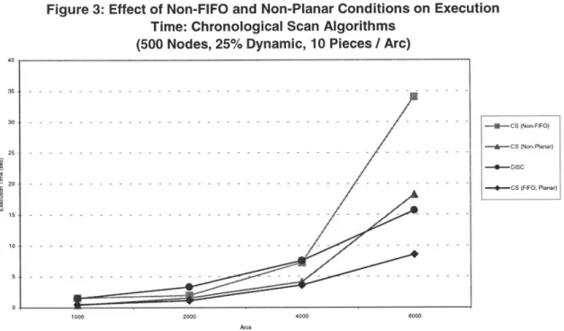
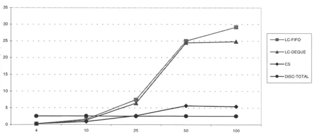
Chapter 8 contains the results of extensive computational testing. The two primary classes of algorithms developed within this thesis, chronological scan algorithms and label-correcting algorithms, are evaluated for a wide range of both randomly generated and real networks, and shown to be roughly equivalent in performance. We also compare the performance of these techniques with that of the best existing discrete-time dynamic shortest path algorithms, and show that in many cases the continuous-time approaches are much more efficient, both in terms of processing time and space.

Finally, we give concluding remarks in Chapter 9, including a summary of the results developed within this thesis, and suggestions for future directions of research.

(12)

Chapter 2 Literature Review

In this chapter, we briefly outline previous results from the literature so as to frame our new results within a historical perspective. Well-known previous results for computing shortest paths within FIFO networks are reviewed. We then discuss methods used to address discrete-time problems; these methods will be compared with new time approaches in later chapters. Finally, existing results which relate to the continuous-time case are reviewed.

2.1 Algorithms for FIFO Networks

It is common for many dynamic networks, for example transportation networks, to satisfy the well-known First-In-First-Out, or FIFO property. This property is mathematically described in Section 3.2; intuitively, it stipulates that commodities exit from an arc in the same order as they entered, so that delaying one's departure along any path never results in an earlier arrival at an intended destination. One of the most celebrated results in the literature on this subject is the fact that the minimum-time dynamic shortest paths departing from a single source node at a single departure time may be computed in a FIFO network by a slightly modified version of any static label-setting or label-correcting shortest path algorithm, where the running time of the modified algorithm is equal to that of its static counterpart. This result was initially proposed by Dreyfus [10] in 1969, and later shown to hold only in FIFO networks by Ahn and Shin [1] in 1991, and Kaufman and Smith [14] in 1993. As many static shortest path algorithms are valid for both integer-valued and real-valued arc travel times, modified static algorithms which solve the minimum-time dynamic shortest path problem from a single source node and departure time can be adopted for dynamic network models in either discrete time or continuous time. Such modified static algorithms are discussed in Section 5.1.

As the so-called "minimum-time one-to-all for one departure time" dynamic shortest path problem in a FIFO network is well-solved, this thesis focuses on the development of

(13)

algorithms for all other common problem variants of the continuous-time dynamic shortest path problem. For the case of FIFO networks, we will discuss methods for computing shortest paths from all nodes and all departure times to a single destination node, and shortest paths from a source node to all destination nodes for all possible departure times, rather than a single departure time. Furthermore, we discuss solution algorithms for problem variants in networks which may not necessarily satisfy the FIFO property, and algorithms which determine paths which minimize a more general travel cost rather than just the travel time.

2.2 Discrete-Time Models and Algorithms

The dynamic shortest path problem was initially proposed by Cooke and Halsey [7] in 1966, who formulated the problem in discrete time and provided a solution algorithm. Since then, several authors have proposed alternative solution algorithms for some variants of the discrete-time dynamic shortest path problem. In 1997, Chabini [3] proposed a theoretically optimal algorithm for solving the basic all-to-one dynamic shortest path problem, and Dean [9] developed extensions of this approach to solve a more general class of problems with waiting constraints at nodes. Pallottino and Scutella

(1998) provide additional insight into efficient solution methods for the all-to-one and one-to-all problems. Finally, Chabini and Dean (1999) present a detailed general framework for modeling and solving all common variants of the discrete-time problem, along with a complete set of solution algorithms with provably-optimal running time.

We proceed to discuss the methods used to model and solve discrete-time problems. Consider a directed network G = (N, A) with n = INI nodes and m = IA I arcs. Denote by dy[t] and cy[t] the respective travel time and travel cost functions of an arc (i,

j)

e A, so that dy[t] and cy[t] give the respective travel time and cost incurred by travel along (i,

j)

if one departs from node i at time t. For clarity, we use square brackets to indicate discrete functions of a discrete parameter. If we want to minimize only travel time rather than a more general travel cost, then we let cj[t] = dy[t]. In order to ensure the representation of these time-dependent functions within a finite amount of memory, we assume they are defined over a finite window of time t e (0, 1, 2, ..., T}, where T is

(14)

determined by the total duration of time interval under consideration and the by granularity of the discretization we apply to time in this interval. Beyond time T, we can either disallow travel, or assume that network conditions remain static and equal to the value they assumed at time T.

It is easy to visualize and solve a discrete-time dynamic shortest path problem by constructing a time-expanded network, which is a static network that encapsulates the dynamic characteristics of G. The time-expanded network is formed by making a separate copy of G for every feasible value of time - its nodes are of the form (i, t), where

i e N and t e (0, 1, 2, ..., T], and its arcs are of the form ((i, t), (j, min{T, t + dy[t]})),

where (i,

j)

e A and t e (0, 1, 2, ..., T), and where the travel cost of every such arc is

given by c,[t]. Since paths through the time-expanded network correspond exactly in cost and structure to paths through the dynamic network G, we can reduce the problem of computing minimum-cost dynamic paths through G to the equivalent problem of computing minimum-cost paths through the static time-expanded network, a problem which we may solve by applying any of a host of well-known static shortest path algorithms to the time-expanded network. However, since the time-expanded network has a special structure, specialized static shortest path algorithms may be employed to achieve a more efficient running time. This special structure is apparent from the construction of the network: there are multiple levels corresponding to the different copies of the network G for each value of time, and no arc points from a node of a later time-level to a node of an earlier time-level. The time-expanded network is therefore "multi-staged" - _{it is acyclic with the exception of arcs potentially connecting nodes}

within the same level of time.

The running time of solution algorithms for the discrete-time problem depends on the problem type, but worst case asymptotic running time is almost always pseudo-polynomial in T (the only significant exception is the aforementioned minimum-time one-to-all problem in a FIFO network, which is solvable in the same amount of time as a static shortest path problem). A discrete-time solution algorithm will typically need to examine a significant portion of the nodes and arcs in the time-expanded network,

(15)

leading to a worst-case lower bound of 2(nT + mT) on running time. This lower bound is also often close to the average-case running time of most discrete-time solution algorithms. Since T usually takes values in the hundreds or thousands, discrete-time approaches can have very high computational demands. Furthermore, the amount of memory required by these algorithms is typically £2(nT) in the worst (and often average) case, as one needs to assign cost labels to the nodes of the time-expanded network in order to compute shortest paths through this network.

Although discrete-time solution algorithms are straightforward to design and implement, they have many drawbacks, including primarily their high storage and processing time requirements. Additionally, the high running time of a discrete-time algorithm often doesn't reflect the true complexity of the dynamics of the underlying problem. For example, consider a problem in which the travel cost of only one arc changes at exactly one point in time. In fact, this is a common scenario, since time-constrained minimum-cost static shortest path problems may be modeled as dynamic problems in which one arc changes its travel cost (to infinity) at exactly one point in time. In order to obtain a solution to this problem using discrete-time methods, one must often do as much work as in a fully-dynamic problem in which all network data is constantly changing - simplicity in the time-dependent network data very rarely translates to a lower running time. Also, in most dynamic networks, a high percentage of the network is actually static. For example, in a transportation network, major roads exhibit dynamic characteristics due to changes in congestion over the course of a day, but lesser-traveled minor roads, comprising a large percentage of the network, are for the most part unaffected by congestion delays and remain essentially static. Discrete-time algorithms typically offer no corresponding decrease in running time as a reward for this simplicity, as their performance is determined for the most part only by n, m, and T, and not by the structure of the time-dependent network data. In contrast, we will see in forthcoming chapters that the performance of the new continuous-time algorithms developed in this thesis will be determined primarily by the complexity of the network data, so that their running time is more closely correlated with the true complexity of a problem, and so that they may solve simple dynamic problems with much greater efficiency.

(16)

2.3 Previous Results for Continuous-Time Problems

The only significant previous algorithmic results in the literature related to the continuous-time dynamic shortest path problem are due to Halpern [12] in 1977, and Orda and Rom [15], [16] in 1990 and 1991. These papers consider the problem variant of computing optimal paths through a continuous-time dynamic network originating at a single source node, where waiting is allowed within certain fixed intervals of time at each node. Halpern considers only the case of computing paths of minimum time, while Orda and Rom consider the more general case of computing paths of minimum cost. They each propose solution algorithms, and argue their correctness and termination within a finite amount of time. The work of Orda and Rom is much more comprehensive than that of Halpern, and identifies problems for which the algorithm of Halpern will fail to produce an optimal solution within a finite amount of time.

The primary shortcoming of the algorithms of Halpern and those of Orda and Rom is that they are presented as theoretical, rather than as practical results. These algorithms rely on operations on general continuous-time functions as their fundamental operations; hence, these algorithms as stated can be prohibitively complicated to implement, let alone implement efficiently. To date no authors have reported on any computational evaluation of these algorithms, except for one case in which the algorithm of Halpern was evaluated for a static network with time windows (feasible regions of time during which one's visit to a node must fall).

There are two primary approaches for creating a feasible implementation of the algorithms of Halpern and of Orda and Rom: either one must discretize time, in which case one enters the discrete-time domain, in which superior algorithms exist, or alternatively one may impose a simplifying piece-wise linearity assumption on the continuous-time network data as is done in this thesis. Under piece-wise linearity assumptions, the methodology underlying the algorithms of Halpern and of Orda and Rom forms the basis for the second of two classes of solution algorithms discussed in this thesis, which we call label-correcting algorithms. In Chapter 7, we describe this broad class of solution algorithms, including the special cases developed by these authors, and

(17)

provide a thorough theoretical analysis of their performance. We show that these algorithms will run in polynomial time in when used to compute minimum-time paths through FIFO networks. The other class of solution algorithms, which we call chronological scan algorithms, is presented in Chapter 6; chronological scan algorithms are shown to have stronger worst-case theoretical running times than label-correcting algorithms.

Ioachim, Gelinas, Soumis, and Desrosiers [13] address the question of computing optimal static shortest paths through an acyclic network in the presence of time windows. Waiting at nodes is allowed during these windows, and accrues a cost which is linear in the amount of time spent waiting. The authors devise a solution algorithm which is relevant to the work in this thesis because it produces piece-wise linear path travel costs. This result may be seen as a very special case of the general framework developed in this thesis, since it is restricted in focus only to static, acyclic networks. The continuous-time dynamic models developed in this thesis provide a more general approach for representing and solving a much wider class of problems, both dynamic and static, involving time windows.

(18)

Chapter 3 Continuous-Time Models

In this chapter, we discuss notation for continuous-time models, and describe the different variants of continuous-time dynamic shortest path problems.

3.1 Piece-Wise Linear Function Notation

The results in this thesis depend strongly on the simplifying assumption that network data functions are given as piece-wise linear functions of time. We assume that all piece-wise linear network data functions have a finite number of pieces, and by convention we treat all points on the boundary between two linear pieces of a function as belonging to the piece left of the boundary, unless the boundary point is itself a linear piece of zero extent. We assume, however, that all network data functions given as input to a dynamic shortest path algorithm will contain only linear pieces of strictly positive extent.

Since there may be several piece-wise linear functions involved with the specification of a single dynamic shortest path problem, we adopt the following general notation for a piece-wise linear functionf(t):

P(f) : Number of pieces into whichf is divided. B(f k) : The right boundary of the kth piece off.

By definition, let B(f 0) = -o and B(f P(f)) = +oo. a(f k) Linear coefficient of the k'h linear piece off.

#(f;

k) Constant term in the k'h linear piece off.

We may therefore specify an arbitrary piece-wise linear function f(t) as follows.

f

()(t) if - oo< t:B(f,1) f 2 _(t) _{if B(fl)<}_t _B(f,2)

f(t) =

f"((t)

if B(f,2)<t B(f,3) (3.1)

f (f(t) if B(f, P(f) -1)< t < +oo

(19)

If some time t marks the boundary between two linear pieces of a function, we say that this function improves at time t if either it is discontinuous and drops to a lower value after time t, or if it is continuous and its derivative drops to a lower value after time t. Likewise, we say that a function worsens at a boundary time t if either it is discontinuous and jumps to a higher value after time t, or if it is continuous and its derivative jumps to a higher value after time t. This terminology is used because in this thesis we will seek the minimum value of a piece-wise linear objective function, and a decrease of this function or its derivative will correspond to an improvement in the objective. It is possible for a piece-wise linear function to both improve and worsen at a boundary point, if both the function and its derivative are discontinuous at that point. For example, the function could improve by jumping to a lower value at time t and simultaneously improve by its derivative jumping to a higher value at time t. Finally, we say that a function is simple over a region if it contains no piece-wise boundaries within that region.

In all of our models, there is no particular significance attached to the time t = 0, or to times which are positive. We will always consider functions of time to be defined over all real values of time, and we will compute solutions which represent network conditions over all values of time. The choice of origin in time can therefore be arbitrary.

3.2 Network Data Notation

Let G = (N, A) be a directed network with n = INI nodes and m = IA I arcs. Let Ai denote the set

(j

I (i,

j)

e A] of nodes after node i, and let B = {i I (i,

j)

e A] denote the set of nodes before node

j.

For each arc (i,

j)

e A, we denote by d1(t) the travel time of a

commodity entering the arc at time t. It is assumed that all arc travel time functions are piece-wise linear, finite-valued, and greater than some arbitrarily-small positive value. On occasion, instead of arc travel time functions, it will be more convenient to work with arc arrival time functions, defined as ay(t) = t + d1(t). We define the quantity P* to be

the total number of linear pieces present among all arc travel time functions: P*= XP(dij).

(3.3)

(20)

We denote by the piece-wise linear function cyj(t) the general cost of traveling along an arc (i,

j)

e A, departing at time t. As time approaches + oo, we assume that all travel time and travel cost functions either increase linearly or remain static and non-negative; otherwise, least-cost paths of unbounded duration may occur. For the same reason, it is also assumed that the initial linear pieces of each arc travel time and arc cost function are constant (and also non-negative, in the case of travel cost); that is, there must be some point in time before which the network is entirely static. This assumption is generally not restrictive in practice, because we are typically only interested in computing optimal paths within the region of time which extends from the present forward.

We say that a function f(t) satisfies the First-In-First-Out, or FIFO property if the function g(t) = t + f(t) is non-decreasing. A piece-wise linear function f(t) will satisfy the FIFO property if and only if a(f k) _> -1 for every k e [1, 2, ..., P(f)] and there are no discontinuities where at whichf(t) drops to a lower value. We describe an arc (i,

j)

e A as a FIFO arc if d1(t) satisfies the FIFO property, or equivalently if ay(t) is

non-decreasing. If all arcs (i,

j)

e A are FIFO arcs, we say that G is a FIFO network. Commodities will exit from a FIFO arc in the same order as they entered, and commodities traveling along the same path in a FIFO network will exit from the path in the same order as they entered. As we shall see, this special characteristic enables the application of efficient techniques to compute minimum-time paths in FIFO networks. Finally, if g(t) represents the "arrival time" function t + f(t) of a FIFO travel time functionf, we define the FIFO inverse of g(t) as:

g_(t) = max {'j. (3.4)

{Tig(r) t)

For any arc (i,

j)

e A in a FIFO network, the arc arrival time inverse function ay~'(t) gives the latest possible departure time along the arc for which arrival occurs at or before time

t. In any FIFO network, arc arrival time inverse functions will always exist, and will themselves be non-decreasing functions of time; we therefore can define the inverse of the arc travel time function dy(t) of an arc as dy-(t) = af-'(t) - t. It can be easily shown that each dy-1(t) function will satisfy the FIFO property and will have the same form as the original dy(t) function - it will be piece-wise linear with a finite number of pieces (no

(21)

more than twice as many pieces as the original function), where each piece spans a duration of time of strictly positive extent. Taking the FIFO inverse of an arrival time function twice yields, as would be expected, the original function.

Depending on the situation being modeled, it may be permissible to wait at some locations in the network during travel along a path. In order to model a general waiting policy in a dynamic network, we must specify two time-dependent quantities: bounds on the length of time one may wait at each node, and the costs of waiting for different lengths of time at each node. Let ubwi(t) be a non-negative-valued piece-wise linear function which denotes the upper bound on the amount of time one may wait at node i following an arrival at time t. We assume that these functions satisfy the FIFO property, because it is sensible for the latest time until one may wait at a node, t + ubwi(t), to be a

non-decreasing function of t. It is not necessary to specify lower bounds on waiting times, since any amount of required waiting time at a node may be incorporated directly into the arc travel time functions of the arcs directed out of that node. Finally, for each node i e N, we denote by WTi(t) the set of feasible waiting times

(

I 0 r ubwi(t)} if waiting begins at time t.

In general, the cost of waiting at a node is a function of two parameters: the starting time and the duration of the interval of waiting. For simplicity, however, we focus in this thesis only on waiting costs which adhere to a simpler structure: we say waiting costs are memoryless if the cost of waiting beyond a particular time is not dependent on the amount of waiting which has occurred up until that time. In this case, one can write the cost of waiting at node i from time t until time t + r as the difference between two cumulative waiting costs, cwci(t + r) - cwci(t), where

cwc,(t) = J w(t)dt , (3.5)

and where wi(t) gives the unit-time cost of waiting density function of node i. We assume that the wi(t) functions are piece-wise constant and non-negative, so that the cumulative waiting cost functions cwci(t) will be piece-wise linear, continuous, and non-decreasing, and so the cost of waiting for any interval of time will always be non-negative.

(22)

Memoryless waiting costs are very common in dynamic network models. If the objective of a dynamic shortest path problem is to find paths of minimum travel time, then waiting costs will be memoryless because they will satisfy cwc;(t) = t. As a final restriction, if waiting is allowed anywhere in the network, and if G is not a FIFO network or if minimum-cost paths are desired, then we require continuity of all network data functions. If this restriction is not met, then an optimal solution may not exist. An example of such a problem is a single arc network, where unbounded waiting is allowed at no cost at the source, and where the travel cost of the single arc (i,

j)

is given by:

CU. (t)=1 if t e (-o,0]

(3.6)

t if t Ce (0,+CO)

In this case, there is no optimal solution. In practice, the continuity restriction is not troublesome, since any discontinuity in a piece-wise linear function may be replaced by an additional linear piece with an arbitrarily steep slope. For problems in which waiting is prohibited, continuity of network data functions is not required.

3.3 Description of Problem Variants

Dynamic shortest path problems may be categorized into different variants based on the criteria used to select optimal paths and on the desired configuration of source and destination nodes and times. As an objective, it is often the case that we wish to find paths of minimum travel time; in this case, cy(t) = dy(t), and we call the problem a minimum-time dynamic shortest path problem. We refer to the more general problem of finding paths of least cost a minimum-cost problem. Optimal paths through a dynamic network may contain cycles, depending on the network data. In FIFO networks, though, we shall see that minimum-time paths will always be acyclic.

As with static shortest path problems, the fundamental dynamic shortest path problems involve the computation of optimal paths between all nodes and either a single source or single destination node. The addition of a time dimension, however, complicates the description of dynamic problems since a "source" now comprises both a source node and a set of feasible departure times from that node, and a "destination" consists of a node along with the set of feasible arrival times at that node. Additionally, there is a greater

(23)

distinction in dynamic problems between computing optimal paths emanating from a source node and computing optimal paths into a destination node. In the realm of static networks, these two problems are made equivalent by reversing all arcs in the network; in dynamic networks, the problems are still related but more remotely so, as there is often no trivial way to transform one to the other. In FIFO networks, however, there is greater degree of symmetry between these two types of problems. We will discuss methods of transforming between symmetric problems in FIFO networks in Section 4.4.

In this thesis, we consider two fundamental variants of the dynamic shortest path problem, which we call the all-to-one and one-to-all problems. The all-to-one problem involves the computation of optimal paths from all nodes and all departure times to a single destination node (and an associated set of feasible arrival times at that destination node). Symmetrically, the one-to-all problem entails the computation of optimal paths from a single source node (and a set of feasible departure times) to all other nodes. There are two common flavors of the one-to-all problem. The most common, which we simply call the one-to-all problem, involves computing a single shortest path from the source node to every other node, where departure time from the source is possibly constrained. The other variant, which we call the one-to-all problem for all departure times involves computing separate shortest paths from the source to every other node for every feasible departure time. An important result, which we discuss in Section 4.4, is the fact that in a FIFO network, the minimum-time all-to-one problem is computationally equivalent to the minimum-time one-to-all problem for all departure times.

The all-to-one problem is of benefit primarily to applications which control and optimize the system-wide performance of a dynamic network, as its solution allows for commodities located anywhere in time and space to navigate to a destination along an optimal route. The one-to-all problem, conversely, is well-suited for applications which compute optimal routes from the viewpoint of individual commodities traveling through a dynamic network from specific starting locations. In this thesis we will develop

(24)

3.4 Solution Characterization

For the all-to-one problem, we designate a node d e N as the destination node. We can then characterize a solution to the all-to-one problem by a set of functions which describe the cost and topology of optimal paths to d from all nodes and departure times. The following functions will constitute the set of decision variables used when computing an optimal solution to the all-to-one problem:

C/l)(t) : Cost of an optimal path to d departing from node i at time t, where waiting is allowed at node i before departure.

C(")(t) : Cost of an optimal path to d departing from node i at time t, where no waiting is allowed at node i before departure.

Ni(t) : Next node to visit along an optimal path to d from node i, time t.

Wi(t) : Amount of time to wait at node i, starting at time t, before departing for node Ni(t) on an optimal path to d.

Based on the information provided by these functions, it is a simple matter to trace an optimal route from any starting node and departure time to the destination, and to determine the cost of this route.

For the one-to-all problem, we designate one node s e N as a source node. We will use an equivalent but symmetric form of notation as in the all-to-one problem in order to describe a solution to the one-to-all problem. Specifically, we characterize a solution by a set of functions which specify the structure and cost of optimal paths from s to all nodes and all arrival times:

C/l)(t) : Cost of an optimal path from s to node i and time t, where waiting is allowed at node i after arrival and up until time t.

C/n")(t) : Cost of an optimal path from s arriving at node i at exactly time t.

PNi(t) : Preceding node along an optimal path from s to node i and time t.

PTi(t) : Departure time from the preceding node PNi(t) along an optimal path from s to node i and time t.

Wi(t) : Amount of waiting time to spend after arrival at node i up to time t

on an optimal path from s.

Specification of both the previous node and previous departure time functions is necessary in order to trace a path from any arbitrary destination node and arrival time back to the source. It is almost always the case that in the one-to-all problem, we are concerned with finding the best path to each node i e N irrespective of arrival time. In

(25)

this case, we can therefore specify for each node i e N the arrival time opti at that node which yields the best possible path travel cost, where

opt = arg min{ C,(w) (t) I Vi e N. (3.7)

Given any destination node i e N, one may use the preceding solution information to easily determine the cost and structure of an optimal path from s to i.

Under the assumption of piece-wise linear network data functions, we shall see that the path travel cost functions C(w)(t) and C/"")(t), the waiting time functions Wi(t), and the previous node departure time functions PTi(t) which comprise the solution to the one-to-all and one-to-all-to-one problems will also be piece-wise linear. To describe the piece-wise linear behavior of these solution functions, we define a linear node interval, or LNI, to be a 3-tuple (i, ta, tb), where i e N, and where (ta, tb] is an interval of time of maximal possible extent during which Ni(t) (or PNi(t)) does not change with time, and during which the remaining solution functions change as simple linear functions of time. For the all-to-one problem and for all problems in FIFO networks, we shall see that LNIs will always span a duration of time of strictly positive extent. However, LNIs comprising the solution to a one-to-all problem may in some cases span only a single point in time - we will call such LNIs singular. The LNI (i, ta, tb) chronologically preceding a singular LNI

(i, tb, tb) at some node i e N is taken to represent the interval of time (ta, tb) which contains neither of its two endpoints.

For each node, it will be possible to partition time so as to divide the piece-wise behavior of departures from that node into a finite number of LNIs. The output of an all-to-one or one-to-all dynamic shortest path algorithm will therefore consist of an enumeration of the complete set of LNIs for every node i E N, along with a specification of the solution functions during each LNI. During the time extent of a particular LNI at some node i, we say that node i exhibits linear departure behavior, as arrivals or departures to or from the node during this interval follow the same incoming or outgoing arc experience an optimal path cost which changes as a simple linear function of time.

(26)

Chapter 4 Problem Formulation and Analysis

This chapter contains a mathematical formulation and optimality conditions for the all-to-one and all-to-one-to-all continuous-time dynamic shortest path problems. Following this, we establish some of the fundamental mathematical properties of solutions to these problems, and we discuss several key properties of FIFO networks. We show that a solution always exists for all variants of the dynamic shortest path problem, and that this solution always consists of a finite number of linear node intervals. In the case of a FIFO network, we will develop stronger bounds on the number of LNIs comprising the solution to a minimum-time path problem. Finally, we discuss symmetries between different variants of the minimum-time dynamic shortest path problem in a FIFO network - we will show that the minimum-time all-to-one problem and the minimum-time one-to-all problem for all departure times are computationally equivalent, so it will be necessary in future algorithmic chapters only to develop solution algorithms for one of these two problems.

4.1 Mathematical Formulation

In order to simplify our formulation of the all-to-one problem, we wish for the destination node d to appear at the end of all optimal paths, but not as an intermediate node along these paths. For minimum-time problems, this is not an issue. In minimum-cost problems, however, we enforce this desired behavior by replacing node d with the designation d'and by adding a new artificial destination node d along with a zero-cost arc (d' d). We assume that arrivals to d at any point in time are allowed; if there are restrictions on the set of feasible arrival times at d, we may model these by setting the time-dependent travel cost of the arc (d' d) so it incurs infinite travel cost at prohibited arrival times. In general, one may only constrain the arrival time for minimum-cost or non-FIFO minimum-time problems, since it is usually not possible to add such a constraint while satisfying the FIFO property.

(27)

The optimality conditions for the general minimum-cost all-to-one dynamic shortest path problem are as follows. A proof of necessity and sufficiency of these optimality conditions appears at the end of this section. In order to ensure optimality, the solution functions C/3)(t) and C(")(t) must satisfy:

Cf")(t) = min {cwcm(t +T _-cwci(t) + C ""l(t +VT) Vi e N, (4.1)

rEWT (t)

C(nw)(t) = min{c0(t)+C )(t+d(t))} if i = d Vi e N. (4.2)

je Ai

At optimality, the solution functions W(t) and Ni(t) are given by arguments respectively minimizing equations (4.1) and (4.2). These functions are not necessarily unique, since there may be several paths and waiting schedules which attain an optimal travel cost.

W1(t) = arg min{cwc,(t+ T)- cwc,(t)+ C(nw)(t +T)} Vi e N, (4.3)

rEWT (t)

N, (t) = arg min{cj (t) + C~w) (t + d j (t))} Vi e N - {d}. (4.4)

je A;

For the one-to-all problem, we take similar steps as in the all-to-one case in order to prevent the source node s from appearing as an intermediate node in any optimal path, in order to simplify the formulation of the problem. For minimum-cost one-to-all problems, we therefore replace s with the designation s'and add a new artificial source node s and a zero-cost arc (s, s'). In order to restrict the set of feasible departure times from s we use the same method as with the all-to-one problem, in which the time-dependent travel time and cost of the arc (s, s') is used to determine the set of feasible departure times. As in the all-to-one problem, restriction of departure times in this fashion only applies to minimum-cost or non-FIFO minimum-time problems. For the minimum-time one-to-all problem in a FIFO network, it is necessary to consider only the single earliest possible departure time, since we shall see in Section 4.3 that departures from later times will never lead to earlier arrivals at any destination.

Optimality conditions for the one-to-all problem are similar to those of the all-to-one problem. Since network data is stored in a so-called "forward-star" representation, from which we cannot easily determine the set of departure times along a link that result in a particular arrival time, we write the optimality conditions as set of inequalities rather than

(28)

minimization expressions. _{If Cif()(t) and Ci/")(t) represent a feasible set of path costs,} then they must satisfy the following conditions for optimality:

C fW(t)+c (t) C5 ""(t + dj (t))' V(i,

j)

e A, (4.5)

CI"n) (t) + cwc, (t + T) - cwc, (t) Cfw) (t + T) VT E WTi(t), Vi e N - [s], (4.6)

CW)"(t) = C"W)(t) = 0. _(4.7)

The functions Wi(t), PNi(t), and PTi(t) must at optimality satisfy the following conditions in a minimum-cost one-to-all problem:

Cf") (t) + cwcj (t + W, (t)) - cwcj (t) = Cfw) (t+W,(t)) Vi E N, (4.8)

C w) (PT (t)) + Cf nw) (t), where I = PN (t) Vi e N- [s}. (4.9)

Proposition 4.1: Conditions (4.1) and (4.2) are necessary and sufficient for optimality for the all-to-one dynamic shortest path problem, and conditions (4.5), (4.6), and (4.7)

are necessary and sufficient for optimality for the one-to-all problem.

Proof: It is a simple matter to show that these conditions are necessary for optimality. If any one of these conditions is violated, then the particular arc or waiting time causing the violation may be utilized as part of a new path in order to construct a better solution. For example, if condition (4.2) fails to hold for some node i e N and time t, then this means there is some outgoing node

j

e At which will lead to a better path than Ni(t). Since violation of these conditions implies non-optimality, the conditions are therefore necessary.

In order to show sufficiency, we examine first the case of the all-to-one problem. Assume conditions (4.1) and (4.2) are satisfied by some functions Ci/w)(t) and Cinw)(t)

which represent a feasible solution. Consider any feasible path from some node i e N and some departure time t to the destination node d, having the form P = (i1, t, w1) - (i2,

t2, W2) - ... - (i, tk, Wk), where each ordered triple represents a node, an initial time at that

node, and a waiting time before departure from that node. We have ij = i, t] = t, i = d, Wk = 0, and for any valid path we must have t1 1 =t1 +w+d, ,,(tj+ w) for all

j

e (1,

(29)

C " (t I ) cwc (t, + wI) - cwcj (t) + C") (t, + wI) (4.10)

C

" (t4) cwc (tI + w,) - cwc (t1 ) + c (t' + w₁) + CW) (t2) (4.11)

In general, after expanding the Cw) (t2) term in (4.11), followed by C(w)(t 3), C(w)(t 4),

etc. along the entire path, since C(,) (t) = 0 the right-hand side of the inequality in (4.11) will expand into the cost of the entire path P. Hence, C/w)(t) is a lower bound on the cost of any arbitrary path from node i and time t to the destination, and since C/l)(t) represents the cost of some feasible path, we conclude that the solution represented by C/w)(t) and C/nw)(t) is optimal. A similar, symmetric argument applies to show that conditions (4.5), (4.6), and (4.7) are sufficient for optimality for the one-to-all problem.

E

4.2 Solution Properties

We proceed to establish several useful mathematical properties of solutions to the all-to-one and all-to-one-to-all dynamic shortest path problem in a piece-wise linear continuous-time network.

Lemma 4.1: There always exists a finite time t', beyond which all nodes exhibit linear departure behavior. Similarly, there always exists a finite time t -Y prior to which all nodes exhibit linear departure behavior.

Proof: We prove the lemma for the all-to-one problem; the same argument applies to the one-to-all problem. Consider first the case of constructing a value of t'. We focus on the region of time greater than all piece-wise boundaries of all network data functions d1(t),

c1(t), wi(t), and cwc;(t), so these functions will behave as simple linear functions for the

interval of time under consideration. We further restrict our focus within this interval to a subinterval of time t > to, where to is chosen such that c1(t) 0 for all arcs (i,

j)

e A.

Such a subinterval always exists since we have assumed that all arc travel cost functions must be either increasing or static and non-negative as time approaches infinity. For any departure at a time t > to, there exists an acyclic optimal path to the destination which involves no waiting, since the introduction of waiting or a cycle can never decrease the

(30)

cost of any path departing at a time t > to. For any node i e N, we can therefore enumerate the entire set of feasible acyclic paths from i to d. There will be a finite number of such paths, and each of these paths will have a simple linear time-dependent path travel cost for departure times t > to. The optimal path travel cost from i to d for departures within this interval will be the minimum of this finite set of linear functions, and since the minimum of such a set of functions will be a piece-wise linear function with a finite number of pieces, there must exist some departure time ti' after which the same path remains optimal forever from i to d. We can therefore pick t' to be the maximum of these ti* values.

The existence of the time t - is argued from the fact that we know by assumption that there is some time tstatic before which the network data functions remain static. One may always find acyclic optimal paths which involve no waiting that arrive within this region of time, since the presence of waiting or a cycle in any path arriving within this time interval can never decrease the cost of the path. We thus have an upper bound of I P(d1,l) on the length of any path which arrives at a time prior to tstatic, so we can (i, j)E A

accordingly set t -to the value tstatic- Y

#(dj,l).

D

(i, j)E A

Lemma 4.2: The time-dependent function giving the optimal travel cost of any particular path P as a function of departure time will always be piece-wise linear, and consist of a finite number of linear pieces, each spanning an extent of time of strictly positive

duration. The function giving the optimal travel cost of any particular path P as a function of arrival time will always be piece-wise linear and consist of a finite number of

linear pieces, where some of these pieces may span an extent of time of zero duration. Proof: Suppose that a path P consists of the sequence of nodes ii, i2, ... , ik. The

time-dependent travel cost along path P as a function of departure time will depend on the waiting times spent at the nodes along the path, and the optimal time-dependent travel cost function is obtained by minimizing over the set of all such feasible waiting times. For simplicity, we will say that a function is special if it is piece-wise linear and consists

(31)

of a finite number of linear pieces, each spanning an extent of time of strictly positive duration. We prove the fact that the optimal time-dependent travel cost function (as a function of departure time) along any path P will be special by induction on the terminal sub-paths of P of increasing number of arcs: ik, ik-1 - ik, ik-2 - ik-1 - ik, etc. We claim that each of these sub-paths is special. The induction hypothesis trivially holds for the path consisting of the single node ik, since this path has zero travel cost. Suppose now that the induction hypothesis holds for some sub-path Pr+ = ir+1, ..., ik. We can write the time-dependent optimal travel cost of the sub-path Pr = ir, ir+1, ..., ik as a function of departure time using (4.1) and (4.2) as follows. We denote the optimal travel cost of such a sub-path at departure time t by TCp,r(t).

TCpr(t) = min {cwc (t _reWr;(t) + T) -cwc,(t)+ci,1 (t + T)+ TC,,+ (ai,, (t +T))} (4.12)

Denote the composition of the path travel cost function TCr+j and the arc arrival time function a, as TC'p,r+i(t). This composed function will be the composition of two special functions, so TCp,r+](t) will also be special. We can then write Equation (18) in the following simple form

TCp,r(t)= min {f,(t+T }-cwc,(t), (4.13)

TEWr;(t)

where fr (t) = CWC (t) + Ci,,1 (t) + TC, r+l (t) is a sum of special functions, and therefore also

special. If waiting is prohibited at all nodes, then we will have TCp,r(t) = fr(t) - cwci(t), which will be special. If waiting is allowed as some nodes, then by the continuity assumption fr(t) will be continuous, and the minimum of fr(t + T) over the window [t, t + ubwi(t)], where the endpoints of this window are continuous non-decreasing functions if t, will also be a special function. We therefore have the fact that TCp,r(t) satisfies the induction hypothesis, and by induction, the optimal time-dependent travel cost of the entire path TCp(t) = TCp,,(t) must be special.

Once the optimal time-dependent path travel cost function TCp(t) is determined as a function of departure time, we can define an associated travel time function TTp(t) which gives the time required to transverse path P, departing from time t, using an appropriate waiting schedule such that we can achieve the minimal path transversal cost TCP(t). It

Continuous-time dynamics shortest path algorithms

Continuous-Time Dynamic Shortest Path

Algorithms

Continuous-Time Dynamic Shortest Path

Algorithms

Abstract

Acknowledgments

Contents

Chapter 1

Introduction

Chapter 2

Literature Review

j)

j)

j)

Chapter 3

Continuous-Time Models

#(f;

f

f"((t)

(j

j)

j)

j.

j)

j)

j)

j)

j)

(

j)

(3.6)

Chapter 4

Problem Formulation and Analysis

j)

j

j

C

j)

#(dj,l).