Controlling physical layer parameters for mobile ad-hoc networks

Controlling Physical Layer Parameters for Mobile

Ad-Hoc Networks

by

Roger Hu

Submitted to the Department of Electrical Engineering and Computer

Science

in partial fulfillment of the requirements for the degree of

Master of Engineering in Electrical Engineering and Computer Science

at the

MASSACHUSETTS INSTITUTE OF TECHNOLOGY

August 2001

L*V) 2

©

Roger Hu, MMI. All rights reserved.

The author hereby grants to MIT permission to reproduce and

distribute publicly paper and electronic copies of this thesis document

in whole or in part.

A uthor ..

...

DeparIment of Electrical Engineering and Computer Science

August 10, 2001

Certified by...

...

Robert Morris

Assistant Professor

ThesiQ. Supervisor

Arthur C. Smith

Chairman, Department Committee on Graduate Students

Controlling Physical Layer Parameters for Mobile Ad-Hoc

Networks

by

Roger Hu

Submitted to the Department of Electrical Engineering and Computer Science on August 10, 2001, in partial fulfillment of the

requirements for the degree of

Master of Engineering in Electrical Engineering and Computer Science

Abstract

This thesis investigates the use of software radios for ad-hoc networking to improve spectrum utilization and battery life. An API that provides a mechanism for a net-work node to request services from the software radio layer and a framenet-work that permits a physical layer to be constructed based on these needs are also presented. In addition, this framework is used to analyze the 802.11 wireless standard to identify some of its limitations.

Thesis Supervisor: Robert Morris Title: Assistant Professor

Acknowledgments

I would especially like to thank my thesis adviser, Robert Morris, for showing me both the patience and enthusiasm to supervise me during this past year. He helped tremendously with the direction and focus of this research.

I am also thankful to Vanu Bose, who took time out of his busy schedule as

CEO and President, to review my rough drafts. He and the other members of Vanu

Inc., including John Chapin, Andrew Chiu, Victor Lum, Steve Muir, Alok Shah, also provided support to develop this thesis. My twin brother Stanley also helped in this regard.

My gratitude also extends to Mingxi Fan and ChangQing Zheng, who shared their

expertise in communications with me. I relied on them to help sort out my confusion while wading through digital communications and spread spectrum books.

Finally, I would also like to thank my parents, for their love and guidance during these past twenty-three years.

Contents

1 Introduction 13

1.1 Limitations in Current W ireless Ad-Hoc Systems . . . . 14

1.2 How Software Radio Overcomes these Limitations . . . . 14

1.3 Related W ork . . . . 15 1.4 Thesis Scope. . . . . 16 1.5 Road Map . . . . 16 2 Background 17 2.1 Overview . . . . 17 2.2 Modulation . . . . 17 2.2.1 Bandwidth Efficiency . . . . 18

2.2.2 Error Performance Curves . . . . 19

2.3 Channel Coding . . . . 21

2.3.1 Block Coding . . . . 21

2.3.2 Convolutional Coding . . . . 22

2.3.3 Coding Gain . . . . 22

2.4 System Operation . . . . 22

3 Software Radio Architecture 25 3.1 Overview . . . . 25 3.2 Framework . . . . 26 3.2.1 Regulatory Limits . . . . 26 3.2.2 Channel Constraints . . . . 27 3.2.3 User Requirements . . . . 27 3.3 Performance Metrics . . . . 27 3.3.1 Latency . . . . 28 3.3.2 Energy Consumption . . . . 28 3.3.3 Data Rate . . . . 29 3.3.4 Probability of Error . . . . 29

3.4 Physical Layer Design . . . . 29

3.4.1 Modulation and Coding Choices . . . . 29

3.4.2 Tradeoffs . . . . 31

3.4.3 Selection Process . . . . 32

3.4.4 Assumptions . . . . 33

4 802.11 Framework 37

4.1 Overview ... ... 37

4.2 802.11 Physical Layer . . . . 37

4.3 Regulatory Constraints . . . . 37

4.4 Frequency Hopping Implementation . . . . 38

4.4.1 Frame Format . . . . 39 4.5 Performance Metrics . . . . 40 4.5.1 Latency . . . . 40 4.5.2 Energy Consumption . . . . 40 4.5.3 D ata R ate . . . . 41 4.5.4 Probability of Error . . . . 41

4.6 Possible Improvements with Software Radio . . . . 41

5 Conclusion 45 5.1 _{Sum m ary . . . .} 45

5.2 Future W ork . . . . 45

6 Appendix 47 6.1 Calculating Minimum Transmit Power . . . . 47

6.1.1 Transmit power for FSK and (207, 187) Reed Solomon . . . . 48

6.1.2 Transmit power for 802.11 2.4 GHz at 200 m . . . . 49

List of Figures

1-1 Mobile ad-hoc network diagram. . . . . 13

2-1 Transformation from bits to waveforms . . . ... 17

2-2 Error performance curves for several modulation schemes . . . . 20

2-3 Possible codeword mapping for a (4,2) block code. . . . . 21

2-4 Hamming distance between two different codewords. . . . . 22

2-5 Coding G ain. . . . . 23

2-6 System Operation Movement. . . . . 23

3-1 Software radio architecture. . . . . 25

3-2 Signal processing chain. . . . . 26

3-3 Energy consumption for different modulation schemes for a node lo-cated 200 meters (400-byte packet transmitting at 2.4 GHz). . . . . 32

3-4 Physical layer design considerations . . . . 32

4-1 Frequency Hopping Spectrum Utilization . . . . 38

4-2 802.11 Frame Format. . . . . 39

List of Tables

2.1 Phase shift mapping for QPSK . . . . 18

2.2 Probability of bit errors for various modulations. . . . . 20

3.1 Constraints imposed by regulation. . . . . 26

3.2 Constraints imposed by the channel. . . . . 27

3.3 Parameters specified by user . . . . 27

3.4 Set of possible modulations and coding schemes. . . . . 30

3.5 Latency and cycles for several different modulation schemes. . . . . . 30

3.6 Latency and cycles for several different coding schemes. . . . . 30

3.7 Latency and energy consumption for DQPSK and different coding schem es. . . . . 31

4.1 Constraints imposed by the FCC. . . . . 38

Chapter 1

Introduction

A mobile ad-hoc network is a collection of wireless nodes that can communicate with

each other without any dependence on a fixed infrastructure or centralized adminis-tration (see Figure 1-1). Nodes within transmission range can communicate directly with each other, but those out of range must rely on other nodes to forward along packets to their final destination. Because they can be deployed quickly and require no extra planning, ad-hoc networks are often useful for establishing temporary work-groups in classroom settings, business meetings, or disaster relief situations[1].

A

Mobile Node

- Wireless Link

Figure 1-1: Mobile ad-hoc network diagram.

Mobile ad-hoc networks have also been widely used for tactical military commu-nication systems. The United States Defense Advanced Research Project Agency (DARPA) has sponsored projects such as the Near-Term Digital Radio (NTDR) sys-tem to control infantry, armor, and artillery units in battlefield scenarios where no communication infrastructure exists[5]. In addition, the current GloMo program is investigating the use of multimedia voice, data, and video traffic with ad-hoc mobile radio networks[9].

1.1

Limitations in Current Wireless Ad-Hoc

Sys-tems

There are several limitations in current wireless ad-hoc network systems, which in-clude the inability to adjust to interference, available bandwidth, and different net-working standard implementations. Because these systems are usually designed for certain channel characteristics, they have difficulty adjusting to different environ-ments. The examples presented below helps illustrate some of these limitations.

A node operating in a crowded lecture hall encounters very different noise and

interference levels than a small classroom. Modulation and channel coding schemes that make efficient use of the available bandwidth should therefore be adjusted to suit these different environments. A node in a crowded lecture hall, for instance, might choose to boost the amount of error correction, while a node in a small classroom might switch to a modulation technique that encodes more data at the expense of a lower tolerance to noise. In current wireless ad-hoc networks, there is very little flexibility to make such dynamic adjustments.

In battlefield situations, infantry and tank battalions are often moving across var-ious terrains and obstacles, causing their communication links to suffer from varying path loss, multipath fading, and signal quality degradation[9]. Because each vehicle acts as a network node and a router, adjustments that can provide additional relia-bility to the communication link need to be done quickly. Current ad-hoc networks focus on improving reliability at the routing layer[14] [13], but do not allow physical layer parameters such as transmit power, modulation, error control rate, and symbol transmission rate to be easily modified.

Another significant problem facing current ad-hoc network systems involves in-teroperability. A wireless device supporting the Bluetooth ad-hoc networking stan-dard cannot exchange data messages with a card supporting the 802.11 stanstan-dard. Similarly, different branches of military and law enforcement agencies have different communication devices that cannot inter-operate with each other, which poses a sig-nificant problem during joint operations such as disaster relief, riot control, and drug

interdiction[ 18].

1.2

How Software Radio Overcomes these

Limita-tions

Software radio technology attempts to perform all the physical and link layer pro-cessing on general purpose processors. A handheld with an analog-to-digital (A/D) converter, for instance, would digitize the RF spectrum of interest and perform the signal processing entirely in software. Dedicated signal processors (DSPs) and ap-plication specific integrated circuits (ASICs) to perform down conversion, low-pass filtering, and demodulation would not be needed.

A handheld device in an ad-hoc network currently has an extremely limited

technology impose too much of a burden to make it practical for today's use. How-ever, with expected advances in low power processors and battery technology, we expect this situation to change in the next three to five years.

There are significant advantages for software radio in ad-hoc networks. Rather than choosing transmission parameters that are suited for certain channel conditions, adjusting transmitter power, modulation, and coding can result in more efficient spec-trum and energy use. Such flexibility in making adjustments provides a tremendous advantage for ad-hoc networks, which typically have ill-defined network boundaries, limited spectral bandwidth, and network topologies that constantly change [1].

1.3

Related Work

Much research in software radio technology has developed from the SpectrumWare project at the MIT Laboratory of Computer Science. The project explored how a software-oriented signal processing approach could be used for wireless communica-tions. A protocol for mobile hosts to coordinate the transition to a different physical layer was developed in [2]. In addition, the design issues of implementing a software-based frequency hopping spread spectrum radio were explored in [15].

In addition, there has been research investigating the design of architectures that can adapt to different heterogenous wireless networks. A handoff system that allows mobile devices to move seamlessly across different networks is introduced in [19]. Although this system allows a user to move from his office to other parts of a building without connectivity being dropped, it requires the individual to bring the equipment that provides the coverage, such as a WaveLAN card or a Metricom Ricochet modem.

A software radio, in contrast, could implement all these standards and eliminate the

need for multiple pieces of equipment.

Research has also focused on different medium access control (MAC) protocols for adjusting transmit power levels. A MAC protocol called Power Controlled Multiple Access (PCMA) proposes to use the signal strength of a received control message to limit the transmit power of nearby stations [10]. The work in [20] explores how power control can also be combined with a multiple channel scheme to provide more efficient spectrum usage, and research by [16] examines how varying power based on node densities can be used for large packet radio networks. Finally, the tradeoffs between MAC retransmission and transmit power are studied in [4]. Other parameters

of the physical layer such as modulation and coding, however, are not considered. In [7], the RTS/CTS protocol is modified in the IEEE 802.11 wireless standard to allow the receiver to choose the rate at which a packet is to be transmitted. The physical layer prefaces every packet with a header, which allows for dynamic rate adjustments. The paper assumes that different modulation schemes can be supported in the physical layer, but does not address how such functionality can be provided.

1.4

Thesis Scope

The goal of this thesis is to demonstrate how software radio technology in ad-hoc networking can improve spectrum utilization and battery life. The design and frame-work of a system that allows a user to specify physical layer parameters based on the current needs of the system is introduced. This framework is then applied to the

802.11 standard and used to identify limitations in this specification.

1.5

Road Map

The next chapter provides a brief introduction about digital communications and discusses how hardware-based radio implementations are limited. Chapter 3 discusses the API and framework that provides parameters to be adjusted in the physical layer.

Chapter 2

Background

In this section, we briefly review the fundamental aspects of digital communications that are important to the design of wireless ad-hoc systems. We discuss the various physical layer parameters such as modulation and channel coding that help determine the overall system performance. Finally, we examine how system operation is affected

by a fixed modulation and channel coding scheme.

2.1

Overview

A signal in a communications system undergoes a series of different transformations

before transmission occurs. The incoming bits are first grouped into symbols, which then map to a finite set of sinusoidal waveforms. The limited number of waveforms allows them to be distinguished by the receiver and translated back into binary digits.

Bits - Symbols No Waveforms

Figure 2-1: Transformation from bits to waveforms.

2.2

Modulation

Modulation is the process in which digital symbols are converted to sinusoidal wave-forms. Varying the amplitude, frequency, and phase allows different waveforms to be created. The general form of these waveforms is represented as follows:

s(t) = A(t) -cos[wot + #(t)] (2.1)

A(t) = amplitude at time t wo = carrier frequency 0(t) = phase at time t

There are several common digital modulation schemes, which include phase shift keying (PSK), frequency shift keying (FSK), and amplitude shift keying (ASK). In these schemes, either the amplitude, frequency, or phase is varied. One form of phase shift keying known as Quadrature Phase Shift Keying (QPSK) varies the phase to represent four different symbols. To represent the symbol '10', for instance, QPSK shifts the phase by 180". Table 2.1 summarizes this mapping.

Symbol Waveform Equation

00 s(t) = A(t) cos[wot]

01 s(t) = A(t) cos[wot + 90']

10 s(t) = A(t) cos[wot + 180']

11 s(t) = A(t) cos[wot + 270] Table 2.1: Phase shift mapping for QPSK

The number of waveforms needed depends on the number of bits used to represent symbols. For instance, QPSK requires two bits to represent four different waveforms. In the general case, if k bits per symbol are used, then 2k waveforms are needed. We

often refer this technique as M-ary signalling, where M equals 2*

Other modulation schemes are variations of phase, frequency, and amplitude mod-ulation. A modulation technique known as Amplitude Phase Keying (APK) varies the amplitude and phase of the sinuosoid to produce different sets of waveforms. In Quadrature Amplitude Modulation (QAM), two amplitude-modulated sinusoids, 900 degrees are out of phase with each other, are used to transmit data.

2.2.1

Bandwidth Efficiency

We can determine the overall efficiency for a particular modulation, expressed as bits/s/Hz, by measuring the number of bits transmitted in a given amount of time divided by the bandwidth used. If there are k bits per symbol and T, represents the duration for a symbol to be transmitted, the data rate can be calculated by dividing these two quantities. The efficiency can then be determined by dividing by the total amount of bandwidth, expressed as Hz, that is used. Equation 2.2 represents this calculation.

R k

-- = bits/s/Hz _(2.2)

W WTS

R = data rate (bits/s)

W = bandwidth (Hz)

k = bits per symbol (bits) T, = symbol duration _(s)

For instance, for MPSK modulation, the bandwidth efficiency is log2M bits/s/Hz

band-width efficiency also increases. The increased bandband-width efficiency, however, comes at a cost of increased bit energy to noise ratio, E.

The bandwidth efficiency can also be used to calculate the maximum data rate that can be supported by the modulation. The bandwidth of the channel can be multiplied by this ratio. For 64-QAM, the theoretical maximum bandwidth efficiency is log1064 = 12 bits/s/Hz. For a 2 MHz channel, the maximum data rate would be

24 Mbps (12 bits/s/Hz - 2 MHz).

2.2.2

Error Performance Curves

An important property of a given modulation technique is the required bit energy to noise ratio

(E)

of 10-5, for instance, means that an error occurs less than once for every 105 bits

transmitted.

The fraction - can be determined by multiplying the received signal strength

with the bandwidth and dividing it by the product of the noise level and data rate. We note that an increase in noise or data rate results in a decrease in . We also observe that -_No increases with signal power and bandwidth. Equation 2.3 represents this calculation:

EbS- = (-)

(2.3)

No N R

S = received signal power (W or dB)

N = noise level (W or dB for a bandwidth of 1 Hz)

R = data rate (Mbps) W = bandwidth (Hz)

If the noise is distributed uniformly across a certain bandwidth, then the

expres-sion simplifies to the following:

Eb- S (-)

(2.4)

No N R

Table 2.2 lists approximated bit error rates for many different types of modulations

[17] [3]. The table is divided into two different columns: coherent and noncoherent

detection. In coherent modulation schemes, the receiver uses knowledge of the phase for detection. Coherent modulation schemes tend to have a lower E requirement for the same probability of bit error than non-coherent modulation schemes, but additional circuitry is required in order to track the signal and usually results in increased complexity and higher cost.

The function Q(x), known as the complementary error function, is defined as follows [17]:

Modulation Coherent detection Noncoherent detection BPSK

Q [

FSK

Q

DPSK Not used in practice 1e

QPSK

Q

I

M-QAM 2(1-M-

Q[

Table 2.2: Probability of bit errors for various modulations.

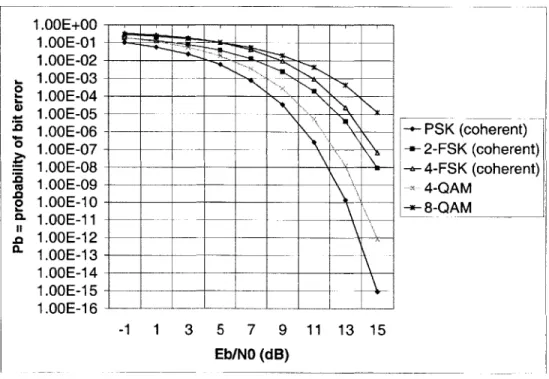
Figure 2-2 is a figure of the plotted error performance curves for various modula-tions, including PSK, 2-FSK, 4-FSK, 4-QAM, and 8-QAM. For any of these perfor-mance curves, we note that reducing the probability of error requires an increase in

. An increase can only occur if a higher transmission power is used or the noise level

No

is reduced. We also observe that the error performance curve for 4-FSK is shifted to the right of 2-FSK, which indicates that performance degrades when encoding more bits per symbol for this particular modulation.

1.OOE+00 1.00E-01 1 .OOE-04 1.OOE-02 1.OOE-03 1.OOE-04 1.OOE-08 0 1.OOE-09 o 1.OOE-07 1.00E-0 o 1.OOE-1 0 0- 1.OOE-1O1 1.OOE-13 IL 1.OOE-123 ~-1.OOE-134 1.OOE-14 1.QOE-15 1.QOE-16 + PSK (coherent) +2-FSK (coherent) +4-FSK (coherent) 4-QAM -8-QAM -1 1 3 5 7 9 11 13 15 Eb/NO (dB)

Figure 2-2: Error performance curves for several modulation schemes.

-I

2.3

Channel Coding

Channel coding refers to the various signal transformations that can be performed to enable transmitted signals to better withstand the effects of various channel im-pairments, such as noise and interference[17]. One form of channel coding is known as forward error correction (FEC), which adds redundant information to data that is being transmitted. There are two major types of forward error correction, which include block and convolutional coding.

2.3.1

Block Coding

Block codes are often referred to as (n, k) codes because an encoder takes a data block of k bits and maps them to a larger block of n bits. The (n - k) bits, which are added

to each data block, are the redundant bits added. These bits are also known as parity or check bits, because they provide a mechanism for error detection or correction.

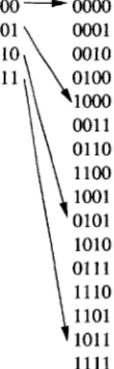
In block codes, there are 2' possible codewords but only 2k sequences that map

to this larger set. In a (4,2) block code, for instance, there are 24 or 16 possible codewords but only 22 sequences. Figure 2-3 demonstrates a possible mapping. An

00 - 0000 01 0001 10 0010 11 0100 1000 0011 0110 1100 1001 0101 1010 0111 1110 1101 1011 1111

Figure 2-3: Possible codeword mapping for a (4,2) block code.

important consideration when choosing an appropriate mapping is the Hamming dis-tance, which is defined as the minimum number of bits that are different between any two codewords in the set. Figure 2-4 illustrates this concept.

A code's ability to detect and correct errors is dependent on the Hamming

dis-tance, since the maximum number of errors that can be detected and corrected is determined by this value. Equations 2.6 and 2.7 specifies the maximum number of errors that can be detected and corrected.

01111

Hamming distance = 4

10001

Figure 2-4: Hamming distance between two different codewords.

ecorrect = d - 1 (2.7)

2

2.3.2

Convolutional Coding

Another type of forward error correction is known as convolutional coding, which uses shift registers and adders to generate codewords. There are two parameters associated with these type of codes: the code rate and constraint length. The code rate, k/n, represents the ratio of the number of bits into the encoder to the number of channel symbols output by the encoder in a given cycle. The constraint length, K, represents

the number of stages in a shift register.

Convolutional codes typically are more powerful, but are much more computation-ally expensive to decode. During the decoding process, the most likely sequence of

possible codewords is chosen, usually using the Viterbi algorithm [17]. An important

parameter of this process is the minimum free distance (df), which affects the number of correctable bits for a convolutional code:

ecorrect = [df 2 11 (2.8)

2.3.3

Coding Gain

The coding gain, expressed as decibels (dB), specifies the difference in E needed to_No achieve the same error probability with a coding scheme. Figure 2-5 illustrates this concept.

In general, convolutional codes have much higher coding gains for the same ratio k/n than block codes. The tradeoff, as mentioned previously, is that convolutional decoding tends to require much more complexity.

2.4

System Operation

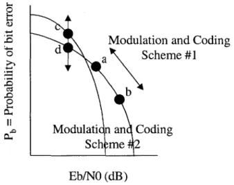
System performance is influenced by the choice of modulation and coding scheme. Movement along the error performance curve results in various tradeoffs. First, in-creasing transmitter power will also cause an increase in _Nor, which helps to improve bit error probability. The tradeoff is shorter battery life because of the higher power

10-2

10-4

10-6

dissipation. This movement Figure 2-6. C C -c C II

is reflected in the movement between points a and b in

Modulation and Coding a Scheme #1

b

Modulati an Coding Sch me 2

Eb/NO (dB)

Figure 2-6: System Operation Movement.

Movements between points c and d, however, require changes to the modulation and coding scheme. As shown in Figure 2-6, a lower error probability might be achievable with a different pair with the same E₀ requirement. Hardware-based radio

implementations do not provide such flexibility. Software radio technology, however, would allow a system's modulation and coding to be changed by programmable means

[17]. Such capability would allow systems to adapt their physical layers to better suit

different environments.

-- (Eb/No)u (uncoded)

(Ej/No)c (coded)

Cckling

in (dB)

Eh/N0

Figure 2-5: Coding Gain. Pb

Chapter 3

Software Radio Architecture

The software radio approach for a physical layer design is presented in this section. We introduce a framework that describes the various considerations that must be made in choose an appropriate modulation and coding pair. Finally, we provide an example of how this framework might be used for ad-hoc network situations.

3.1

Overview

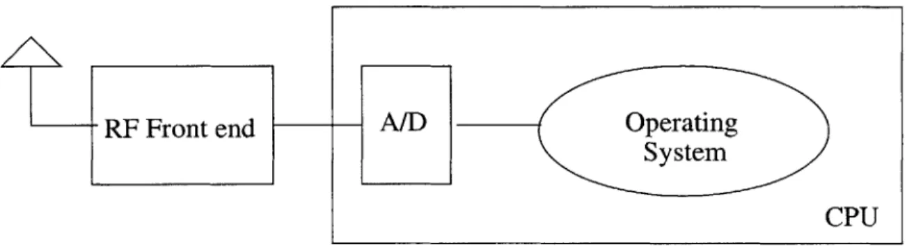
The proposed approach is to perform much of the signal processing tasks of the physi-cal layer in software. An RF frontend takes a wideband of spectrum and downconverts it to an intermediate frequency (IF), which can then be sampled by an A/D converter. The samples can then be processed in the operating system. Figure 3-1 illustrates this architecture.

RF Front end A/D Operating

SystemD

CPU

Figure 3-1: Software radio architecture.

All modulation and coding schemes are implemented as modules. Each of these

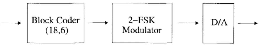
modules, instantiated as a C++ class, can then be connected into a signal processing chain. Figure 3-2 demonstrates an example of a signal processing chain that could be created.

Because of this modular design, a range of modulation and channel coding schemes can then be supported. A change from 2-PSK to 2-FSK modulation, for instance,

sim-ply requires the two different modules to be substituted. The substitution can occur by disconnecting the input and output ports of the original module and reconnecting

it to the new module.

Block Coder (18,6)

,0 2-FSK -p D/A

Modulator

Figure 3-2: Signal processing chain.

3.2

Framework

There are three major categories that impose constraints on the selection of an appro-priate modulation and coding pair: regulatory limits, channel conditions, and user requirements. Regulatory limits are relatively static, while channel conditions and user requirements often vary in ad-hoc network situations. We discuss each of these categories in further detail.

3.2.1

Regulatory Limits

In the United States, regulatory limits are imposed by the Federal Communications Commission (FCC). The set of rules and regulations are described in Title 47 in the Code of Federal Regulations (CFR), which establish maximum power emission limits and specify harmful interference levels. Part 15.247 concerning the 902-928 MHz, 2400-2483.5 MHz, and 5725-5850 MHz bands also contain provisions about the use of spread-spectrum technology. Constraint Bandwidth TX Power Variable BW Ptx Units hertz (Hz) watts (W) Table 3.1: Constraints imposed by regulation.

The major regulatory limits that affect the selection of modulation and coding scheme are maximum bandwidth and maximum transmission power. Limits on band-width affects the achievable data rate, while limits on transmission power places con-straints on the maximum signal strength that can be received. We represent these terms as BW and Ptz, respectively. Table 3.1 summarizes these constraints.

3.2.2

Channel Constraints

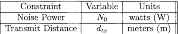
The Shannon-Hartley capacity theorem provides insight into the maximum data rate of a channel. Capacity is defined as bits/s and depends on the signal-to-noise ratio (SNR) and bandwidth (W). Equation 3.1 represents the upper bound on the maxi-mum achievable data rate, assuming that the only noise present in the system can be modeled as a Gaussian process.

C = Wlog₂ + S) (3.1)

We observe that only bandwidth and the signal-to-noise ratio (SNR) affects the achievable data rate. Maximum bandwidth is constrained by regulation, as we noted in the previous section. The signal-to-noise-ratio, on the other hand, is affected by several factors, including the current noise and interference level, transmit distance, and attenuation that occurs during signal propagation.

Constraint Variable Units

Noise Power No watts (W)

Transmit Distance dt meters (m)

Table 3.2: Constraints imposed by the channel.

3.2.3

User Requirements

Varying applications will have different degrees of tolerance for latency, data rate, error rate, and energy consumption. For instance, a bit error rate of 10-3 is considered acceptable for a voice link but 10-7 may be required for a data link. We summarize these varying constraints in Table 3.3.

Constraint Variable Units

Latency Tuser s/packet

Data Rate Ruser bits/s

Bit Error Rate Peuser bit errors/ total bits

Energy Consumption Pdus,,, joules/packet Table 3.3: Parameters specified by user.

3.3

Performance Metrics

We use these four constraints to help define the amount of latency, energy consump-tion, data rate, and probability of error for a given modulation and coding pair. A

user's specified requirements is compared with the set of available of combinations to find a an appropriate match.

3.3.1

Latency

Latency is defined in terms of the processing delay of a packet through the physical layer. In dedicated signal processing systems, incoming samples arrive at a constant rate and are processed with a fixed delay between when a sample enters the system and when the output based on that sample leaves [8]. In a software radio based architecture, such guarantees may not be possible because virtual memory, multiple levels of caching, and competition for the I/O may add jitter to the expected amount of time for a sample to be processed.

The latency, however, can still be approximated by evaluating the amount of time it takes to process the coding and modulation on a packet. We then add the propagation delay to this sum, which is dependent on the packet size and the data rate. The latency per packet for a given modulation and coding, denoted as TL, is

therefore represented in Equation 3.2.

TL = (Tmod + Tcoding) * Npacket + Npacket (3.2)

R

where Tmod and Tcoding represents the amount of seconds needed to compute the

mod-ulation and coding per bit, Npacket equals the number of bits per packet, and R refers to the data rate in bits per second.

3.3.2

Energy Consumption

Another important metric is the amount of energy needed to compute and send a packet. The total energy depends on several factors, including data rate. Data rate influences how long the transmitter must remain on, so a faster data rate results in less energy needed. For instance, assuming 30 mW is used for transmission, the amount of energy needed to send a 1500-byte packet at 1 Mbps is 360 PJ. At 9600 bits/s, the amount of energy needed is 38 mJ.

Energy consumption also depends on the amount of time needed to compute the coding and modulation for the packet. We can represent this value by multiplying the nominal core power of a processor by the cycle count and clock period of the processor. The amount of energy consumed, therefore, is defined in Equation 3.3.

Pd = P - (x NRket) + Pprocessor, CLK -(Cmod + Ccoding) * Npacket (3.3)

where Ptx equals the transmit power level in watts, R represents the data rate in bits/s, Pprocessor represents the average power dissipation of the processor in joules per second, CLK equals the clock period of the processor (seconds/clock cycle), Cmod

and Ccoding is the cycles needed to compute the modulation and coding per bit, and

3.3.3

Data Rate

The maximum data rate that can actually be achieved is bounded not only by the Shannon capacity limit but also the modulation and coding scheme used. A mod-ulation has a certain bandwidth efficiency, defined as bits/s/Hz, so the fastest that can be achieved is simply this value multiplied by the total amount of bandwidth available.

The effective data rate is reduced by the amount of overhead needed to transmit the packet. The ratio Npayoad represents the fraction of bits used for the payload, and coding rate R, represents the percentage bits not used for error correction. Thus, the maximum data rate can be expressed as follows:

Rmax = Bee f iciency - BW - Npayloa- R (3.4)

Npacket

where Befficiency represents the bandwidth efficiency in bits/s/Hz, BW equals the bandwidth in Hz, Npayloa equals the number of bits in the payload, and Npacket is the number of bits in the packet, and Rc refers to the percentage of bits not used for error correction.

3.3.4

Probability of Error

The final constraint is the probability of error, which measures how often a packet has to be retransmitted. The probability of error for a chosen moduation and channel code can be determined by calculating -_No and using its associated error performance curve. The calculated E will be a function of transmitted power, noise power, and

No

distance.

Pe = Pb ktx, No, dtx) = Pb (3.5)

No

3.4

Physical Layer Design

The framework presented can be used to control physical layer parameters that more accurately reflects current channel conditions and user requirements. In this section, we discuss the various tradeoffs involved in selecting an appropriate modulation and coding pair.

3.4.1

Modulation and Coding Choices

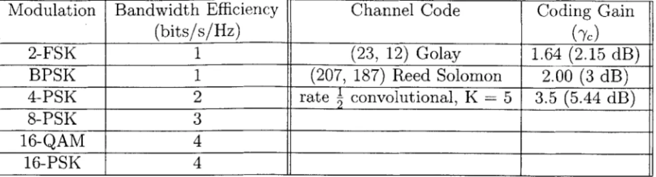
Tables 3.4 shows a set of possible modulation and coding schemes that might be supported. The maximum theoretical bandwidth efficiency, which defines the most number of bits that can be transmitted per hertz, is included for the modulation schemes. An upper bound of the coding gain, which defines the reduction in 1 _No to

achieve the same level of probability with an uncoded modulation technique, is noted for each of the channel codes.

Modulation Bandwidth Efficiency (bits/s/Hz)

Channel Code Coding Gain (Yc) 2-FSK 1 (23, 12) Golay 1.64 (2.15 dB) BPSK 1 (207, 187) Reed Solomon 2.00 (3 dB) 4-PSK 2 rate ] convolutional, K = 5 3.5 (5.44 dB) 8-PSK 3 16-QAM 4 16-PSK 4

Table 3.4: Set of possible modulations and coding schemes.

Several modulation and coding schemes were implemented as C++ modules and benchmarked with the GNU profiler. The profiling program generates information about how much time each module spends processing a sample, which can then later be used to determine the total amount of latency and amount of power consumed per bit. Tables 3.5 and 3.6 shows several of these benchmarked values performed on a Pentium III 1 GHz machine.

Modulation Latency Cycles

2-FSK 8.89 ps/sample (8.89 ps/bit) 8890 cycles/bit DQPSK 2.24 ps/sample (1.12 ps/bit) 1120 cycles/bit Table 3.5: Latency and cycles for several different modulation schemes.

In order to calculate the total latency for a packet, the latency first needs to be converted to cycles per bit. For modulation schemes, the sample size depends on the number of bits used to encode a symbol. 2-FSK, for instance, processes one bit per sample. DQPSK, on the other hand, processes two bit per sample.

Since a (n, k) channel code processes k bits at a time, the number of seconds per bit can be calculated by dividing the latency by k. For the (23, 12) Golay code, for

instance, the latency per bit is equal to 22.2 ns/bit (266.67 ns/sample

/

Coder Latency Cycles

(23, 12) Golay 266.67 ns/sample (22.2 ns/bit) 222 cycles/bit

(207, 187) Reed Solomon .107 ms/sample (572 ns/bit) 5721 cycles/bit

-, K = 5 convolutional 7722.57 ns/sample (7722.57 ns/bit) 7722.57 cycles/bit

Table 3.6: Latency and cycles for several different coding schemes.

The cycles needed to compute the modulation or coding scheme can be determined

by first dividing the number of bits processed per sample by the total time spent to

process the sample. The clock speed of the processor divided by this value then yields the number of cycles per bit. For 4-PSK, the number of cycles is equal to 112 cycles/bit (1 GHz

/

/

/

ns/sample)).

3.4.2

Tradeoffs

There are various tradeoffs to consider in trying to satisfy the equations presented in the framework. Increasing data rate reduces latency and energy, but causes the probability of error to increase. Increasing transmit power comes at the expense of battery life, but reduces the probability of error. Finally, the various computational requirements have different effects on latency, energy consumption, data rate, and probability of error. We consider the various options in this section.

Data Rate vs. Probability of Error. Increasing the data rate decreases both

latency and energy consumption. The data rate determines the propagation delay for a packet, so doubling the rate causes the delay to decrease by the same amount. Energy consumption is also slightly decreased, because the transmitter stays on for less amount of time. The latency and energy consumption for DQPSK and various coding schemes with different data rates (assuming a 400-byte packet transmitting at

30 mW on a Pentium III 1 GHz machine) is shown in Table 3.7.

Modulation/Coding 9600 bps 1 Mbps

DQPSK (uncoded) 336.9 ms / 39.0 pJ 31.6 ms / 35.9 pJ DQPSK/(23, 12) Golay 337.6 ms/110.0 pJ 75.0 ms/106.9 pJ DQPSK/(207, 187) Reed Solomon 355.2 ms / 1869.7 pJ 25.1 s/1866.6 pJ

Table 3.7: Latency and energy consumption for DQPSK and different coding schemes.

Increasing the data rate, however, comes at the expense of probability of error. We note from Equation 2.3 that increases in data rate also causes the E to lower by_No the same amount. For BPSK modulation, doubling the data rate causes the - ratio to decrease by a factor of two.

Transmit power (Pt,) vs. Probability of Error. Because - is proportional

to the received signal power (as expressed in Equation 2.3), an increase in transmitted power causes the probability of error for a chosen modulation and coding scheme to decrease. This improvement, however, comes at the expense of energy.

Figure 3-3 charts the probability of error versus power dissipation requirements for a node transmitting to another node located 200 meters apart at 2.4 GHz. The required received signal power, after accounting for distance (see Appendix 6.1), is used to determine the minimum amount of power needed to transmit for a particular modulation scheme. The number of joules needed for this transmission is then added to the number of joules needed to perform the computation, as specified in Equation

4000 ,. . 3500-- - - ---3000 . 2500 t 2000 DQSK 1500 1000 0

1.OOE-02 1.OOE-03 1.00E-04 1.00E-05 1.00E-06 1.OOE-07 Pb = probability of bit error

Figure 3-3: Energy consumption for different modulation schemes for a node located 200 meters (400-byte packet transmitting at 2.4 GHz).

Latency and Energy Consumption vs. Probability of Error.

Convolu-tional codes tend to produce coding gains for probability of errors at 10' of between 4.0-5.0 dB. In contrast, block codes, which include both Reed Solomon and Golay codes, produce about 2.0-4.0 dB coding gains [3]. However, as shown in Tables 3.4 and 3.6, the improvement comes at a cost at both latency and energy. A (24, 12) Golay code requires 222 cycles/bit, while a rate 1 convolutional code requires approx-imatley 10157 cycles/bit. Channel codes which produce higher coding gains, which translate to a lower probability of error, tend to require more processing.

3.4.3

Selection Process

User Requirements _Modulation

Regulatory Limits

Channel Conditions Coding ,

Figure 3-4: Physical layer design considerations.

We propose a method for choosing a particular modulation and coding pair. First, the physical layer must be provided with the following information: desired data rate,

bit error rate, latency, and power dissipation. This information is then incorporated with the regulatory limits and channel conditions, as shown in Figure 3-4.

The next step is to choose a coding/modulation pair with the bandwidth efficiency and coding rate that could support the required data rate. We then use equation 3.2 to see if the pair meets the user imposed latency constaint. If the inequality is not satisfied, then we choose another pair and start over the process.

If the latency equation is met, the next step is to determine the transmit power

required. Because all of the parameters in inequality 3.5 are known except for Pt, we can determine the minimum transmit power required to meet the probability of error constraint by solving for Pt_.

The value calculated for Pt, can be used to check that the power constraint of inequality 3.3 is met. If not, then several options can be considered. The first is to lower transmit power at the cost of causing a higher bit error rate. The second option is to increase data rate at the expense of probability of error. Alternatively, the power constraint can be relaxed. Lastly, a different modulation and coding scheme might be attempted.

If there is no pair that adequately meets the requirements, then a metric for

deciding the closest match might be needed. One option, for instance, is to minimize the bit error rate at the expense of the other parameters.

3.4.4

Assumptions

There are several assumptions in this framework. First, the choice of a particular modulation scheme often depends on other characteristics besides their maximum theoretical bandwidth efficiency. Quadrature Amplitude Modulation (QAM), for in-stance, tends to be more susceptible to amplitude and phase distortion than PSK or FSK [12]. The choice of modulation, therefore, may need to include other factors besides maximum data rate.

Second, calculating the minimum transmit power based on the required E _No is assumed to minimize power dissipation. Lower transmit power, which results in higher bit error rates, may cause more packet retransmissions that the amount of energy consumed may be higher than transmitting at a higher power level [4]. In addition, the optimal transmit power may actually be to choose an algorithm that delivers a constant, pre-determined amount to the intended receiver [16].

Finally, the distance is assumed to be known by using the received signal strength from a previous transmission exchanged between the nodes. If this previous transmis-sion incurs significant multipath distortion, the amplitude of the signal may provide an incorrect estimate of distance. In addition, the two nodes may not have commu-nicated previously or may not know about each other's existence.

3.4.5

Example

Suppose that the maximum bandwidth available (BW) is 500 kHz, maximum

trans-mit power allowed (Pt,) is 1 watt, noise level (No) equals 2.00.10-17 W, and the

tolerable latency (TLu,,r), maximum power dissipation (Pds,,,), minimum data rate (Ruser), and the minimum bit error rate (peuser):

Maximum latency (TLu,,,) = < 70 ms per packet

Maximum energy consumption (Pdue) < 5.4 mJ per packet

Minimum data rate (Ruser) > 115,200 bps

Minimum BER (pe,,,,) > 10-5

From the available modulation and coding schemes listed in Table 3.4, we first try choosing 2-FSK and the rate ! convolutional code. The maximum data rate that₂ can be supported by this particular pair (assuming the payload comprises of entire packet) can be calculated using Equation 3.4. Since this value is equal to 250,000 bps, the modulation can support the required data rate.

1

Rmax = 1bits/s/Hz -500kHz. 1 --2 250,000bps

The latency constraint specified in 3.2 is first checked to see if it meets the user's requirements (assuming a 400-byte packet):

TL = (Tmod + Tcoding) -Npacket + Npacket

3200bits

- (8.89 ps/bit + 7722.57ns/bit) -3200bits + 1200bs

115, 200bps

= 80.9ms/packet

Because the user has requested a latency of less than 70 ms, this modulation and coding pair is not appropriate. The next step is to find another pair that does meet this constraint. 2-FSK and a (207, 187) Reed Solomon coder would be one candidate, since it has a calculated latency of approximately 56.3 ms and maximum data rate of 452 kbps.

The next step would be to determine the minimum transmit power. For FSK, the approximate E for a bit error rate of No 10-5 based on Figure 2-2 is equal to 12.5 dB, or 17.78. With a (207, 187) code that provides a 3.0 dB coding gain, this ratio translates into approximately a transmit power of 50.1 mW (see Appendix 6.1.1)

The next step is to see if the power constraint is held. The processor that performs the modulation and coding is assumed to be a Pentium III 1 GHz machine with an average power dissipation of 100 mW. Using 3.3, the amount of energy consumed would be calculated as follows:

= 50.1 -10-3W 3200bits + 100. 10-3_W.

( 1 (8890 + 5721cycles) - 3200

115, 200bps 10 9_cycles/s

= 6.07mJ

Because this amount is too large for the user's specified requirement, we have several options. The first is to try a different modulation and coding pair, which would mean to restart the entire process. The second option is to attempt to increase the data rate to reduce the amount of energy consumed during transmission.

However, increasing the rate from 115,200 bps to 192,000 bps results in a 2.2 dB change (10logio 192000 - 10logio 115200). This rate change would drop the error probability from 10-5 to 10-4 (according to Figure 2-2). However, even with this rate

change, energy consumption is only reduced to 5.51 mJ, which still does not meet the user requirements.

The next option is to try to recalculate the minimum transmit power needed for a lower error probability, such as 10-'. The resulting amount would be 23.1 mW, which would result in a total energy consumption of 5.31 mJ. Therefore, for this particular modulation and coding scheme, the probability of error and/or data rate would need to be sacrificed to reduce the energy consumption.

Chapter 4

802.11 Framework

4.1

Overview

In this section, we evaluate the advantages that a software radio might provide to the

802.11 wireless LAN standard. We use the framework to help identify areas which

have limited flexibility and discuss some of the tradeoffs involved.

4.2

802.11 Physical Layer

There are three different specifications for the 802.11 physical layer: frequency hop-ping spread spectrum (FHSS), direct sequence spread spectrum (DSSS), and infrared. The frequency hopping spread spectrum operates by transmitting a short burst on one frequency and then changing to another short period of time in a predefined pat-tern known only to both the transmitter and receiver [1]. A direct sequence spread spectrum system, on the other hand, distributes the energy of the signal over a large bandwidth. Infrared systems, in contrast, vary the intensity of the current in an infrared emitter.

4.3

Regulatory Constraints

The Federal Communications Commission (FCC) imposes many regulation limits on the unlicensed 2.4 GHz band, which is designated in the United States for indus-trial, scientific, and medical (ISM) purposes. Many different wireless LAN standards, including 802.11, operate over this band for transmitting and receiving data. As a result, systems which use the 2.4 GHz band must be designed to handle any possible sources of interference.

The FCC also imposes limits on transmit power. For devices that do not em-ploy spread spectrum technology, a maximum transmit power of .75 mW is allowed. Frequency hopping and direct sequence systems, which are forms of spread spectrum technology, are limited to 1 watt[6].

Table 4.1 lists the bandwidth and transmit power limitations imposed by the FCC. However, there are also other regulatory constraints that pertain only to frequency hopping spread-spectrum devices. First, frequency hopping devices are allowed to occupy at most 5 MHz of bandwidth. They must also "hop" across a minimum of

15 channels which span across a total of 75 MHz in bandwidth. Finally, the system

must not spend more than 400 ms in a particular channel within a 30 second period.

Constraint Value

Bandwidth (BW) _{75 MHz (direct sequence spread spectrum)}

5 MHz (frequency hopping spread spectrum)

TX Power (Pt,) 1 W (spread spectrum)

.75 mW (non spread-spectrum)

Table 4.1: Constraints imposed by the FCC.

4.4

Frequency Hopping Implementation

The 802.11 frequency hopping implementation divides the 2.4 GHz band into 78 frequencies, each occupying 1 MHz of bandwidth (see Figure 4-1). A pseudorandom generator defines the hopping sequence pattern, which consists of 26 channels. The maximum time spent in any channel is specified for 224 ps.

.e. t3 I' I' 'I I' I ~ I ~ I ~ I ~ t2 I' I' I' Ii I' I' I ~ to ti I' I' I' I ~ I ~ I ~ I ~

1 MHz

2.483 GHz

Figure 4-1: Frequency Hopping Spectrum Utilization.

To achieve the 1 Mbps and 2 data rates, a modulation scheme known as Gaussian Frequency Shift Keying (GFSK) is used. GFSK is a form of frequency modulation (FM), in which different symbols are represented by variations in the carrier frequency. The major difference is that GFSK modulation first filters the binary data with a

2.400 GHz

pulse-shaping filter. This filter is needed in order to limit the bandwidth of the signal to 1 MHz.

The 802.11 standard supports up to eight transmit power levels, but there is no specific requirement. Instead, the standard states that an implementation which uses a transmit power of more than 100 mW must also support one power level below that amount. In many FHSS wireless LAN cards, transmit power is fixed at 100 mW.

Data Rate 1 Mbps (2-GFSK)

2 Mbps (4-GFSK) Transmit Power Up to 8 different levels

(if one level > 100 mW, another must be < 100 mW)

Hopping Sequence 3 sets of 26 channels (minimum hop distance of 6 channels) Table 4.2: Frequency Hopping Parameters.

4.4.1 Frame Format

The frame format defines how data is transmitted at the physical layer. It contains information about the type of modulation and data rate employed, in addition to a field that specifies the length of the payload. Figure 4-2 contains a diagram of the format.

Preamble Header

Sync SFD Signal Sevice Length CRC-16 Payload 128 bits 16 bits | 8 bits 8 bits 16 bits 16 bits (Variable)

1 or 2 Mbps transmission

(2-GFSK or 4-GFSK)

:41

Figure 4-2: 802.11 Frame Format.

The frame is divided into three sections: preamble, header, and payload. The preamble includes the synchronization and start of frame delimiter, which is used

by the receiver to detect the presence of a signal. The header provides information

about the type of modulation and data rate that will be used to send the payload, in addition to the size of the payload. Finally, the payload includes the data that needs to be transmitted.

I

4.5

Performance Metrics

The feasibility of implementing a software-based frequency hopping system has al-ready been demonstrated in [15]. However, the benefits for ad-hoc networks has not been closely examined. In this section, we apply the framework and discuss areas in which a software radio architecture could provide additional benefits.

4.5.1

Latency

The header and payload are transmitted separately. While the header is always transmitted with a fixed modulation and data rate, the payload can be transmitted at 1 or 2 Mbps data rate. As a result, the latency for sending the preamble and header is 192 ps.

Modules for GFSK and CRC-16 were also implemented and benchmarked on a Pentium III 1 GHz machine. The computational cost for GFSK modulation is about 8.89 ps/bit (8890 cycles/bit), while CRC-16 takes approximately 1708.9 ns/bit

(1708.9 cycles/bit). The latency, therefore, can be represented as follows:

TL = (TGFSK - TCRC-16) -Npacket + 192ps + Npacket

TL = (8.89ps/bit + 1708.98ns/bit) -Npacket + 192ps + Npacket

R TL = (10.5 - ps/bit) - Npacket + 192ps + Npacket

R

where Npacket equals the number of bits per packet (usually 3200 bits), and R refers to either 1 or 2 Mbps.

4.5.2

Energy Consumption

Additional power is required to keep parts of an 802.11 network card active for trans-mission or reception [4], but we only consider the energy consumption for sending a packet. There are actually two separate transmissions that take place, since the header and payload are sent separately. The amount of energy consumed can be represented as follows:

Pd = P -(N cket) -+ Pprocessor CLK- (CGFSK + CCRC-16) 'Nacket (4.2)

t.-(NPRket + Pprocessor CLK- (8890cycles/bit + 1708.9cycles/bit) -Npacket

where Pt equals approximately 100 mW, R represents 1 or 2 Mbps, Pprocessor is

assumed to be 100 mW, CLK equals 10' s/clock cycle (for a Pentium III 1 GHz), CGFSK and CCRC-16 is the cycles needed to compute the modulation and coding per

bit, and Npacket equals the number of bits per packet (usually 3200 bits).

4.5.3

Data Rate

The 802.11 standard uses a fixed transmission symbol rate of 1 Msymbols/s, but varies the modulation scheme with either 2-GFSK and 4-GFSK. Therefore, the maximum data rate is either 1 or 2 Mbps. No forward error correction is used, so the coding rate R, equals 1. The effective data rate can therefore be represented as follows:

Rmax = lor2Mbps - Npayload (4.3)

Npacket

where Npayload equals the number of bits in the payload and Npacket equals Npayload

plus 128 bits for the preamble and header.

4.5.4

Probability of Error

The error performance curves for 2-GFSK and 4-GFSK are plotted using MATLAB in Figure 4-3 (See Appendix 6.1.3). GFSK modulation has a parameter known as the modulation index, which is defined as the frequency separation for representing different symbols multiplied by the data rate [24]. In 2-GFSK, this modulation index is set to .32, which means that the frequencies used to represent a logical '0' and '1' are separated by 320 kHz (.32 - 1 Mbps). In 4-GFSK, the average modulation index is .144, which means the frequencies to represent the different symbols are separated

by 288 kHz (.144 - 2 Mbps) [11].

4.6

Possible Improvements with Software Radio

There are several ways that flexibility in a software radio might provide additional benefits. We discuss each of these possibilities in this section.

Higher Data Rates. A header is always sent at 1 Mbps before the payload, incurring a minimum of 192 ps (192 bits

/

to allow different data rates to be supported. Because transmitting at 2 Mbps is considered quite unreliable for frequency hopping spread spectrum systems except in optimal quality conditions, supporting 4-GFSK modulation is consider an optional requirement [21]. As a result, this extra latency provides no major benefit.

A software radio-based implementation, on the other hand, might be able to take

advantage of the existing support in the 802.11 standard to vary the modulation and data rate. Unfortunately, the number of modulation schemes that can be supported is quite limited because coherent detection is hard to maintain. The receiver must reacquire phase lock each time after a hop takes place [17], which is difficult because