Vlasov gyrokinetic simulations of ion‐temperature‐gradient driven instabilities

HAL Id: hal-01804646

https://hal.univ-lorraine.fr/hal-01804646

Submitted on 1 Jun 2018

HAL is a multi-disciplinary open access

archive for the deposit and dissemination of

sci-entific research documents, whether they are

pub-lished or not. The documents may come from

teaching and research institutions in France or

abroad, or from public or private research centers.

L’archive ouverte pluridisciplinaire HAL, est

destinée au dépôt et à la diffusion de documents

scientifiques de niveau recherche, publiés ou non,

émanant des établissements d’enseignement et de

recherche français ou étrangers, des laboratoires

publics ou privés.

Vlasov gyrokinetic simulations of

ion-temperature-gradient driven instabilities

G. Manfredi, M. Shoucri, R. Dendy, A. Ghizzo, P. Bertrand

To cite this version:

G. Manfredi, M. Shoucri, R. Dendy, A. Ghizzo, P. Bertrand. Vlasov gyrokinetic simulations of

ion-temperature-gradient driven instabilities. Physics of Plasmas, American Institute of Physics, 1996, 3

(1), pp.202-217. �10.1063/1.871846�. �hal-01804646�

Vlasov gyrokinetic simulations of ion-temperature-gradient driven instabilities

G. Manfredi, M. Shoucri, R. O. Dendy, A. Ghizzo, and P. Bertrand

Citation: Physics of Plasmas 3, 202 (1996); doi: 10.1063/1.871846 View online: https://doi.org/10.1063/1.871846

View Table of Contents: http://aip.scitation.org/toc/php/3/1 Published by the American Institute of Physics

Vlasov gyrokinetic simulations of ion-temperature-gradient driven

instabilities

G. Manfredi

UKAEA Government Division, Fusion (UKAEA/Euratom Fusion Association), Culham, Abingdon, Oxon, OX14 3DB, United Kingdom

M. Shoucri

Centre Canadien de Fusion Magne´tique, Varennes, Que´bec J3X 1S1, Canada

R. O. Dendy

UKAEA Government Division, Fusion (UKAEA/Euratom Fusion Association), Culham, Abingdon, Oxon, OX14 3DB, United Kingdom

A. Ghizzo and P. Bertrand

LPMI, Universite´ de Nancy-I, 54506, Nancy, France ~Received 28 June 1995; accepted 13 September 1995!

An Eulerian code that solves the gyrokinetic Vlasov equation in slab geometry is presented. It takes into account the E3B and polarization drifts in the plane perpendicular to the magnetic field, and kinetic effects in the parallel direction. The finite Larmor radius is modelled by a convolution operator. The relation is established between this model and others proposed previously, and they are shown to be equivalent in the limit of long wavelengths and small Larmor radii. The code is applied to investigate ion-temperature-gradient modes in the quasi-neutral regime, with adiabatic electrons. Numerical results are reported for a wide range of parameters, including density and temperature profiles, magnetic field strength, and ion to electron temperature ratio. Normally the plasma evolves towards long wavelength structures, although in some cases~when Landau damping is very weak! more strongly turbulent regimes are observed. Test particles are used to compute diffusion coefficients both in real space and velocity space. For the most strongly turbulent regimes, particle diffusion coefficients are of order 20 m2s21. The saturation mechanism is also investigated. Many previous numerical results obtained with particle codes are confirmed, but the Vlasov Eulerian technique allows a much finer resolution of structures both in real space and velocity space.

@S1070-664X~96!03001-6#

I. INTRODUCTION

Ion Temperature Gradient instabilities ~ITG! belong to the vast class of drift instabilities.1 These involve electro-static, low frequency waves which, under particular condi-tions such as the presence of a density or temperature gradi-ent, may become unstable. Their growth rate and saturation level are both generally quite low, a circumstance that ren-ders their numerical simulation a difficult task, for the genu-ine instability must be separated from the underlying numeri-cal noise. This is particularly true for gyrokinetic particle-in-cell~PIC! simulations, whose high noise level has been long recognized. Fluid simulations do not suffer from this limita-tion, but they of course do not incorporate kinetic effects, which may play a crucial role ~see however the recent at-tempt to include kinetic phenomena in a fluid description, by Hammett and coworkers2– 4!. Physically, ITG instabilities may play an important role in explaining the anomalous heat and particle transport observed in tokamaks.5–11There is in-deed increasing evidence from large scale gyrofluid and gy-rokinetic simulations12,13that there is a good match between transport inferred from models of ITG-driven turbulence and measured transport in the core and confinement regions of magnetic fusion plasmas.

ITG instabilities are also called hi-modes, because the

crucial parameter ishi5d ln Ti/d ln ni. Analytic estimates

5 give a critical value ofhi.1, above which these modes are

unstable, and predict ~in the case of slab geometry! that the growth rate is proportional to the cube root ofhi. However,

these estimates are valid only within special ranges of the parameters~namely, forh_i@1! and neglect important effects such as Landau damping, and of course all nonlinear phe-nomena.

The goal we address in this paper is a systematic numeri-cal investigation of ITG instabilities in a shearless slab, using a gyrokinetic Vlasov code. In Vlasov ~Eulerian! codes,14 –16 the phase space is covered with a regular, uniform mesh, and the Vlasov equation is solved by means of a splitting algo-rithm. Although they consume more time and memory than the more popular PIC codes, Vlasov codes have the advan-tage of an extremely low level of noise. This feature allows us to obtain high resolution of coherent structures both in real space and in velocity space. Improved understanding of this aspect of plasma turbulence can thus be expected from these simulations, notwithstanding the simple slab geometry that has been used.

Some preliminary results on hi-modes obtained with

Vlasov codes were published in previous articles.15,16Here, however, we make use of a slightly different model, in which the electrostatic potential is derived from the quasi-neutrality relation, instead of solving the Poisson equation. This allows us to work in the regimel_D!r_i~wherer_iis the ion Larmor radius and lD the Debye length! which is more relevant to

tokamak fusion experiments. Results of previous PIC simu-lations, using a model very close to the one adopted in the present paper, were published by Lee and Tang.17,18 More recently, Cohen et al.19 investigated the effect of velocity shear on ITG modes, again via PIC simulations. In our study, a velocity shear will also be present, induced by the effect of finite ion Larmor radius.

A second goal is to compare the gyrokinetic model that we have used with other models previously proposed in the literature.20,21 These models differ essentially from ours in the treatment of the polarization drift and the finite ion Lar-mor radius correction. However, they can be shown to be equivalent when certain, rather natural, conditions are ful-filled. It is hoped that the work presented here will contribute to the process of comparing and benchmarking numerical models of plasma turbulence in tokamaks, which is at present under way.

The paper is organized as follows. In the next section, we present the mathematical model and its relation to other, previously published, models. Conservation laws are also de-rived. Section III contains a brief analysis of the linear theory, as a guideline for the forthcoming simulations. In Sec. IV, we present the numerical results of the nonlinear evolution, and Sec. V deals with the computation of transport coefficients, such as the particle diffusion coefficients in real and velocity space. These results are discussed in Sec. VI, where we draw our conclusions.

II. THE GYROKINETIC SLAB MODEL

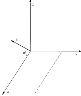
We consider a two-dimensional plasma slab, periodic along the x ‘‘poloidal’’ direction, and non-periodic in the y ‘‘radial’’ direction. The plasma is supposed to be homoge-neous in the z ‘‘toroidal’’ direction~i.e. k_z50!. The external magnetic field is uniform and lies in the (x,z) plane, making an angleuwith the x axis. The geometry of the simulation is sketched in Fig. 1.

The ion gyrokinetic Vlasov equation takes the following form: ]Fi ]t 1“'–@~VWE1VWp!Fi#1Vi“iFi1 e mi E_i* ]Fi ]Vi50, ~1a! VWE5 EW *3BW B2 , ~1b! VWp5 1 ViB dEW_'* dt [ 1 ViB

F

]EW_'* ]t 1~VWE1VWp1VWi!–“EW'*

G

, ~1c!

where V_i5eB/m_i, F_i5F_i(x, y ,V_i,t) and EW52“w. Note that we have explicitly introduced the polarization drift in our model. We also remark that~1c! is an implicit definition of the polarization drift, since Vpappears on the RHS of this

relation: this fact will prove to be useful in the derivation of the energy integral. Appendix A gives further details of the numerical code used to solve Eq. ~1a!.

The asterisk appearing in Eq.~1! is a short-hand for an integral operator that takes into account the finite Larmor radius correction. Following Knorr et al.,22,23we have, for a function h(rW), rW[(x,y):

h*~rW![

E E

G~rW2rW₁!h~rW₁!drW₁[G_*h. ~2!

Equation~2! defines a convolution operator with kernel G(rW) and is more easily represented in wavenumber space:

h*_~kW!5G~kW!h~kW!; G~kW!5exp

S

2k' 2 ri

2

2

D

, ~3! wherer_i5V_thi/V_i is the ion Larmor radius, and, in our ge-ometry, k_'25k_x2sin2u1k_y2 ~see Fig. 1!. This, rather general, expression for the Larmor radius correction is derived by gyrophase averaging, and further assuming a Maxwellian distribution for the perpendicular velocity.22

In order to close the system of equations~1!, we need a further relation, given by the quasi-neutrality constraint

n_i*_5ne, ~4!

where n_i(x, y ,t)5*F_idV_i and the electrons are taken to fol-low the adiabatic law

ne5n0 exp

S

ew Te

D

.n0

S

11ew Te

D

. ~5!

The asterisk in Eq.~4! again stands for the operation defined in Eq. ~2!. Thus, n_i* is the particle density, while ni is the

guiding center density. It can readily be shown that the sys-tem of equations ~1!, ~4! and ~5!, with the prescription ~3!, and appropriate boundary conditions, possesses the follow-ing energy invariant:

W5mi 2

E E E

FiVi 2_dV idrW1 e 2

E E

ni*wdrW 1_2Bmi2

E E

niu“'w*u2drW. ~6!

Details of the calculation of this invariant are given in Ap-pendix B. The first and second term in Eq. ~6! represent respectively the parallel kinetic energy and the electrostatic energy. The third term can be written as (mi/2)**VE2drW and

corresponds to the kinetic energy associated with drift mo-tion.

Slightly different gyrokinetic models have been pro-posed elsewhere in the literature.20,21It is therefore instruc-tive to consider the relation of these models to the one used in this paper. The main difference lies in the treatment of the polarization drift, which is explicitly introduced in our Vla-sov equation @Eq. ~1a!#, while other models take it into ac-count in a modified form of the Poisson equation. Let us first rewrite Eq.~1! in the following way:

d dt log Fi2 1 ViB d dt ¹' 2 w*1 e mi E_i*] log Fi ]Vi 50, ~7! where d dt[ ] ]t1~VWE1VWp!–“'1Vi“i.

We note, before continuing, that both in the original Eq.~1! and in the derivation of Eq. ~7!, we have used an approxi-mation, which we now justify. Strictly, the integral operator

G, defined in Eq.~2!, does not commute with the advective

derivative d/dt, because of the presence of terms like (VW_E1VW_p)–“_'. As illustrated in Ref. 20, Eq.~1! is obtained by assuming the distribution function to be Maxwellian in the perpendicular velocity, and then averaging all terms in

V_' space with a weight J₀(k_'V_'/V_i), J₀ being a Bessel function. This procedure works rigorously for all terms, ex-cept those arising from the nonlinear part of the polarization drift: VW_E–“EW_'. For this term we have, assuming, for sim-plicity, that the magnetic field is parallel to the z axis:

VWE–EW_'52zˆ3“

E_'2

2 . Then averaging over V_',

2zˆ3

E

J0

S

k_'V_' Vi

D

“ E' 2 2 e 2V_'2_/2T d V' 2 2 52zˆ3

S

G_*“ E' 2 2

D

52zˆ3“

S

G* E_'2 2

D

52zˆ3EW_'**–“EW_'**. ~8!

In the last equality, we have defined:

E_'**2_[G

*E_'2. ~9!

Thus our Eq.~1c! is rigorous only if in the nonlinear term we replace E_'* by E_'**. However, it is easy to show that, to leading order in ri, E_'*2_2E '**25ri 2

F

1 2 ¹ 2_E '21EW'–¹2EW'

G

, ~10!

which shows that, for long wavelength~k_'r_i!1!, the correc-tion is of order k_'2ri2. Now, since further analysis will show

that this term is already of higher order in rs/Ln!1

~Ln21[“n/n!, we can safely neglect this correction if we are

interested only in lower order terms.

Returning to Eq.~7!, we perform the following transfor-mation on the distribution function:

Fi5F˜i exp

S

¹_'2_w* ViB

D

~11! yielding ]F˜i ]t 1~VWE1VWp!–“'F ˜ i1Vi“iF˜i1 e mi E_i* ]F ˜ i ]Vi50. ~12! The quasi-neutrality equation becomes

n0 exp

S

ew T_e

D

5G*exp

S

¹_'2 w ViB

D

E

F˜idVi [G*exp

S

¹' 2_w ViB

D

n˜i. ~13!

Expanding the exponentials in Eq.~13! and neglecting terms of order higher than k2r_i2, we obtain finally

ni¹_'2w ViB 2ewn0 Te 5n02

S

11 ri 2 2 ¹' 2

D

_n i. ~14!

It is also usual to replace the ion density on the left hand side of Eq. ~14! with its mean value n0. Now, if we take for instance Eq.~41! in Ref. 20, and expand the modified Bessel functionG0(s)

G0~s![I0~s!e2s.12s, ~15!

where s5k2ri2, we recover our Eq.~14! to the relevant order.

To perform dimensional analysis, we need to introduce the drift-wave ordering as follows:

ef T_e; rs L_n5e!1, vi* Vi 5k'rs rs L_n;e 2_, ~16! rsk';e, rski5cosukxrs;e2, for u'p/2.

Here, v_i* is the usual ion diamagnetic frequency, and

rs5CsVi21, where Cs is the sound speed

A

Te/mi.

Equa-tions ~16! imply that the plasma natural scale is comparable to Ln5~“n/n!21, and much larger than the ion Larmor

ra-dius. This can be true if the typical length in the x direction satisfies Lx*Ln, and if an inverse cascade takes place

to-wards long wavelength structures. Numerical simulations will confirm this point, although during the initial transient of the evolution, structures with a wavelength of order rs

may appear.

By making use of Eqs.~16!, it can be shown that terms in Eq.~1! scale as follows:

]Fi ]t ;e 2_,VW E–“'Fi;e 3_1e¯5_, Ei ]Fi ]vi;e 3_1e¯5_,V i“iFi;e2, ~17! “'–~VWpFi!;~e51e¯7!1~e61e¯8!1~e41e¯6!.

In the polarization term, the first parenthesis refers to the linear part of VWp~proportional to]EW_'/]t!, the second

paren-thesis refers to the term VWE–“EW_', and the third one to the

term VWi–“EW'. The implicit term VWp–“EW'has been neglected

~note however that this term is mandatory to preserve energy

conservation, as shown in Appendix B!. The bar over some of the terms is just short-hand to indicate that these terms come from the finite Larmor radius correction, which is of order k_'2ri

2

. Note also that we have so far considered a case in which Ti5Te, and thusrs5ri: assuming a different

scal-ing for the temperature ratio would result in additional order-ings. From Eqs.~17!, we see that the nonlinear polarization drift VW_E–“EW_' is of higher order, and therefore its Larmor radius correction is negligible, as we had anticipated in our previous discussion.

It is interesting to note that the Vlasov equation as writ-ten in Eq. ~12! is in a characteristic, non-conservative form, and therefore more suitable to be implemented in a PIC code. On the other hand, the form of Eq. ~1! is conservative, and suits best the philosophy of Vlasov Eulerian codes. This is probably one reason why two different models have been chosen for different numerical implementations. However, we have seen that under quite natural assumptions, the two models must coincide.

III. LINEAR ANALYSIS

In this section we sketch some results obtained from linear theory. Since we shall use a simplified model, and drop several terms, we do not expect these results to be directly comparable with simulation results. However, they will pro-vide a useful guideline in designing our computer experi-ments. Let us consider the Vlasov equation~1!, in which we neglect finite Larmor radius and polarization drift effects, coupled to the quasi-neutrality condition, Eq.~4!. We expand all quantities in Fourier series:

Fi~x,y,Vi,t!5F0~y,Vi!1

(

k Fk~y,Vi!e2i~vt2kx!, ~18! w~x,y,t!5w0~y!1

(

k wk~y!e 2i~vt2kx!_,

where k stands for kx5(2p/Lx)n, and n is an integer. We

now introduce the normalization that will be used in this section and in all the subsequent numerical simulations. Time is normalized to the inverse ofV_i5eB/m_i, velocity is normalized to C_s 5

A

T_e/m_i, space is normalized to

rs5Cs/Vi, and the potential is normalized to Te/e. All

nu-merical values are understood to be expressed in these units. With this notation the equilibrium quantities appearing in Eq.

~18! are F0~y,Vi!5 n0~y!

A

2pT~y!exp

S

2 V_i2 2T~y!

D

, ~19! w0~y!50.

Here n₀(y ) and T(y ) are the density and initial temperature profiles. The equilibrium potential is zero since, at t50, we

have ni5ne5n0: a non-zero equilibrium potential could be present, had we considered a finite ion Larmor radius.

With the help of Eqs ~18! we arrive at the desired dis-persion relation n0~y!1

E

]F0/]Vi v/ki2Vi dVi2tanu

E

]F0/]y v/ki2Vi dVi50, ~20!

where k_i5k cosu. In order to investigate the long wave-length behaviour, we expand the denominator ~v/ki2Vi!21 and carry out the integrals. Resonance effects at Vi5v/ki, which give rise to Landau damping, are neglected here, al-though not of course in our full numerical treatment. Finally we arrive at the dimensionless expression:

3Ts42hi22 2 tanu L_n Ts 3_1s2₁tanu L_n s2150, ~21!

where s5ki/v!1,hi5d log T/d log no. From Eq. ~21! we see that a[tanu/Ln is a crucial parameter. Several limiting

cases can be analyzed from Eq. ~21!. For very small s

v5vi*[~k'rs

2_/L

n!Vi,

where k_'5k sinu, and we have restored dimensional units. When a!1, we recover sound waves v5Cski. It is also clear that, in order to obtain unstable solutions, a temperature gradient~i.e. a non-zero hi! must be present.

The caseh_i@1 is particularly interesting. Keepingaand

T fixed, we can neglect the term in s4. The result is a third

degree algebraic equation that admits an unstable solution with:

Res;Ims;

S

1

ahiT

D

1/3

or, in terms of the dimensional frequency

Im

S

v Vi

D

5 2₎ 3

S

a 2 hirs T_i Te

D

1/3 kirs, ~22! Re

S

v Vi

D

52

S

a 2 rshi Ti Te

D

1/3 kirs.

A little algebra shows that the left hand side of Eq ~22! yields:

v;~vi*Cs

2

k_i2hi!1/3 ~23!

as obtained, for example in Ref. 5.

Another interesting case is the flat density profile, for which L_n→`, h<sub>i</sub>→`,a→0, but L_T is finite. Equation ~21! reduces to

T

8

tanu

2 s

3_2s2_{1150 ~24!}

(T

8

5dT/dy), which possesses an unstable root when

T

8

tanu.4)/9. This means that for u approaching 90°, an unstable solution always exists, even for a very small tem-perature gradient. The growth rate, in the regime where

T

8

tanu@1, is given by Imv52) 3

S

T

8

tanu 2

D

1/3 ki. ~25!

Restoring dimensional quantities, Eq.~25! can be expressed in a form similar to that of Eq.~23!:

v;~v_*T_iCs 2 k_i2hi!1/3, ~26! wherev *T_i5 k'ri 2_V i/LT.

IV. NUMERICAL RESULTS

In this section we perform extensive numerical simula-tions of the ITG modes, by varying the crucial physical pa-rameters involved in the governing equations. The model used throughout this section is the one described by Eqs.~1! to ~5! in Sec. II, and the density and temperature profiles adopted throughout this paper are:

n0~y!5N0

H

12 Dn 2 @12tanh~bny!#

J

, ~27! T~y!5T_i0

H

12DT 2 @12tanh~bTy!#

J

.

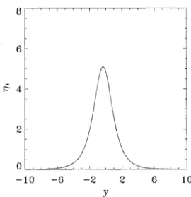
The density profile is fixed for the electrons and also consti-tutes the initial ~guiding-center! density for the ions. The temperature profile intervenes in the ion initial condition as illustrated by Eq.~19!. Note that these profiles do not give a constant Ln21 or LT21, but have a bell-like shape as shown in

Fig. 2. The maximum is reached at y50, where Ln215Dnbn/(22Dn). This fact will render the comparison

with analytical results more cumbersome, but has the advan-tage of being more easily implemented numerically, since the

profiles become flat at y56`, and the plasma can be sup-posed to be homogeneous outside the computational box. The instability is started up by adding a small perturbation

~with an amplitude e.1023_{! to the first three modes of the}

ion density in the x direction.

In the first group of simulations, we consider both a density and temperature gradient, thus yielding a finite hi.

The physical parameters, expressed as usual in dimension-less form, are:

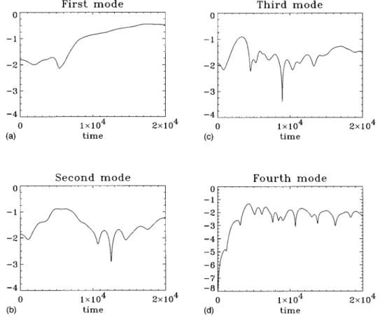
FIG. 3. Time evolution of the modes of the electrostatic potential foru588°, Lx525 and mode k052p/25~a!; Lx525, mode 2k0 ~b!; Lx550, modes

k052p/50~solid line! and 2k0~broken line! ~c!; Lx550, modes 3k0~solid line! and 4k0~broken line! ~d!. Here, and in the following, the scale is logarithmic

in base ten.

T_i05T_e; u588°; D_n50.3; b_n50.4;

DT50.7; bT50.8

giving a maximum value of hi56.1(Ln.14,LT.2.3). The

numerical parameters must be adjusted according to the natural space and time scales of the system. Equation ~22! can be used to determine the order of magnitude of a typical frequency. With the above physical parameters we obtain v;0.02Vi for the fundamental mode k052p/Lx

52p/25.0.25. Accordingly, we have taken a time step

ViDt54. The computational box is as follows: 0,x,Lx;

2Ly,y,Ly; 2Vmax,Vi,Vmax, with Lx525rs or

Lx550rs, Ly510rs, Vmax55Cs. The number of points in

each direction is Nx3Ny3Nv532380310052.56310 5

. This gives a resolution of Dx50.78rs,

Dy50.25rs50.11LT, DVi50.1Cs. For this value of

u588°, Landau damping provides an effective source of

dis-sipation, which allows such a relatively low spatial resolu-tion.

A very common feature, observed in many fluid and ki-netic simulations of plasmas13,24 as well as in laboratory experiments25, is the so-called inverse cascade. Small scale vortices are created in the transient regime, but they rapidly coalesce to give rise to larger vortices, and finally only large scale structures persist. In other words, the system selects the longest wavelength allowed by the imposed boundary condi-tions. In order to check the existence of this phenomenon, we have performed two simulations with, respectively, Lx525rs

and Lx550rs. In Fig. 3 we show the time evolution of

sev-eral modes of the electrostatic potential uwk(t)u integrated

over the y direction. For the case Lx525rs, the first mode

~rsk052prs/Lx.0.25) saturates around Vit53000, while

higher order modes remain at a lower level after saturation. For the case Lx550rs, the second mode ~with now

k150.25! initially dominates, saturating around t56000, but finally, after a long plateau, it drops quite abruptly at

t513000. Meanwhile the first mode ~k050.125! has

satu-FIG. 4. Contour plot and three-dimensional view of the potential at the end of the simulation foru588° and Lx525 ~a! and Lx550 ~b!.

FIG. 5. Wavenumber spectrum of the electrostatic potential, integrated along the non-periodic direction, at time t512000. The scale is logarithmic in base ten. The straight broken line has a slope20.18 log k.

FIG. 6. Time evolution of the modes of the electrostatic potential foru589.5° and Lx525. The plots correspond to wavenumbers k052p/25~a!; 2k0~b!; 3k0

~c! and 4k0~d!.

rated at t514000, and remains dominant in the subsequent evolution. A contour plot of the potential at the end of the simulation ~Fig. 4! shows that, in both cases, a large scale structure survives. The wavenumber spectrum of the electro-static potential integrated over y ~shown in Fig. 5! seems to obey an exponential law 102mk ~with m.0.18! from the early stage of the simulation: subsequently, the spectrum is found to be stabilized and only small fluctuations persist. This rapid fall of the spectrum is quite unusual, compared to the power law behaviour of fluid turbulence, and invites fu-ture investigation. As a first step towards an explanation, we note that Landau damping affects both high and low wave-number structures, while collisional damping is localized in the high k part of the spectrum. This simple fact could pre-vent the existence of an inertial range of wavenumbers in which the mechanism for dissipation can effectively be ig-nored. Finally, we note that, in these simulations, the distri-bution function in velocity space ~not shown here! has un-dergone little change. The evolution is therefore essentially linear, as far as the parallel velocity non-linearity is con-cerned.

As a second example, we study a case for which

u589.5° and Lx525, while all other parameters are the same

as in the previous simulation. With this value of the angleu, the ratio of the poloidal to the toroidal magnetic field is

Bx/Bz5kx/kz5tan21u50.0087, and the parallel

wavenum-ber is ki/kx5cosu50.0087. We also havea5tanu/Ln.8.1.

The first modes of the electric potential are shown in Fig. 6. Comparing with the previous case u588°, we remark that the third and fourth harmonics undergo a very fast initial growth ~note that only the three first modes were initially perturbed with an amplitude e50.001!. However, these higher order modes quickly saturate, and, in the long run, the fundamental mode k052p/Lx becomes dominant. This

be-haviour can be explained as follows. High wavenumber modes would be the most unstable ones in the absence of Landau damping, as shown by Eq.~22!. However, for small enough values of u ~corresponding to larger k_i and hence lower parallel phase velocity! Landau damping prevents these small scale structures developing, while foru close to 90° they can dominate the initial evolution. Note that an angle of u587° must already be considered as small, since we have observed that virtually only the fundamental mode survives. In fact, for the parameters of the previous simula-tions, the parallel phase velocity computed from the numeri-cal results is v/kiVth.0.64 when u588° and v/kiVth.2.5

whenu589.5°. Foru585°, and the same parameters as used above, all modes are damped, and the system is stable.

Returning to the caseu589.5°, Fig. 7 presents a contour plot and a tridimensional view of the electrostatic potential at various times. We note the formation of small wavelength structures at the initial stage of the simulation. The final state is definitely more strongly turbulent than in the caseu588°. This is a general feature we have observed in these and other examples: as the angleuapproaches 90°, a strongly turbulent regime, with short wavelength vortices, begins to appear. For this reason, we often added a small dissipative term of the form n¹_'2F_i to the Vlasov equation, Eq.~1a!. In the present case we have n5531025V_ir_s2. In addition, we have

in-creased the resolution in the x direction, which we found to be most affected by the small scale structures, taking

N_x3N_y3N_v5128380380. It is important to note that the

most severe constraint on N_v does not come from accuracy, but from the recurrence time t52p/k_xDV cosu. This is the reason why for u'90° we can take a smaller number of points in velocity space. In Fig. 8 we show the electrostatic potential, now averaged along the x direction. The initial potential is non-zero because of finite Larmor radius effects

FIG. 8. Electrostatic potential, averaged along the x direction, for the same case as Fig. 6: t50 ~a!; t52250 ~b!; t511250 ~c!.

~remember that in our model the potential is proportional to

the fluctuating part of the ion density!. The potential in-creases in the early stage of the simulation, then it relaxes to an almost constant value ~actually, there is a slight steady growth, but this is due to the small dissipation term, which progressively flattens the ion density gradient!. This modifi-cation in the mean potential cannot be due to the E3B drift

~which, combined with the adiabaticity law, yields no net

current across the magnetic field!. However, in the presence of a finite Larmor radius and polarization drift, transport in the y direction is allowed, and the potential profile can evolve.

Another important question is the mechanism that pro-vides saturation of the ITG instability. This is addressed in Fig. 9, which shows the density and the parallel pressure

p_i5nT_i, averaged along x, as a function of y , at the begin-ning and at the end of the simulation. We see that the initial steep pressure profile becomes considerably smoother, whereas the density profile undergoes little change. The sys-tem thus evolves to a state in which a sys-temperature gradient

~although now a stable one! still exists.

In order to investigate the importance of the viscosity term, we have repeated our first simulation~u588°, Lx525!

for a longer time~V_it516000!, in two cases wheren50 and

n5531025_{respectively. The plot of the Fourier modes~Fig.}

10! shows that they are little influenced by a small viscosity. However, things are quite different in the y direction, due to the presence of a density gradient, as we anticipated earlier. The potential, averaged along x, is presented in Fig. 11 for both cases. Whenn50, the potential stays at a low level, and takes on a ‘‘Mexican Hat’’ shape. When n.0, the viscosity flattens the density profile, which departs more strongly from the equilibrium profile n0, resulting in an increase of the potential. The shape of the potential profile remains close to the initial one, although at a higher level. This simple fact— that viscosity can enhance the electric field in the presence of a density gradient—could be an important issue in edge plasma physics, where all these ingredients play a crucial role.

The growth rates obtained in the previous simulations are smaller than the analytical estimate, Eq. ~22!, which gives Imv;0.0186V_ifor the typical parameters of our first simulation and for the fundamental harmonic. This discrep-ancy is mainly due to Landau damping and finite Larmor radius effects~the latter also acts to reduce the growth rate!, which are not included in the calculations leading to Eq.

~22!: indeed, our order-of-magnitude calculation for the

par-allel phase velocity, yielding v/k_iV_th.2.5, proves that

Lan-dau damping is not negligible even for u589.5°. We also note that the growth rates that we compute are not local, since they are averaged over the non-periodic direction, and

FIG. 9. Pressure profile~a! and density profile ~b! as a function of y, at t50

~solid line! and at t513500 ~broken line!.

FIG. 10. Modes of the electrostatic potential for n50 ~solid line! and

n5531025_{~broken line!, for a simulation withu588°, L}

x525,hi.6. The

that our value ofhi is a function of y ~see Fig. 2!. As a test

for the accuracy of the code, we have thus performed a simu-lation with u590° and ri50.15rs. In this case, the density

profile is stable, and the plasma oscillates at the diamagnetic frequencyv_i* _{5 kx}r_s2_V

i/Ln. The theoretical frequencyvi*

5 0.0178Vi is very close to the frequency observed in the

simulation.

In order to investigate the effect of a finite Larmor radius on the instability, we have performed a simulation with the following dimensionless parameters:

Lx525; u588°; Dn50.3; bN50.4;

DT50.7; bT50.8; ri50.4rs.

These are identical to the parameters of our first simulation

~see Fig. 3!, except for the smaller ion Larmor radius. We

also added a viscosityn5331024. The time evolution of the first four modes~Fig. 12! shows a very rapid growth of the third and fourth harmonics, resulting in a more strongly tur-bulent regime. Generally speaking, effects due to the finite perpendicular ion temperature seem to play an important role in stabilizing small scale structures.

We now consider the case of a flat density profile, n₀51. In this situation, the smoothing operation that accounts for the finite ion Larmor radius@Eq. ~2!# has no effect, at least

initially, on the ion density ni(t50)5n051. Thus we can expect behaviour close to that observed when ri!rs, i.e.

enhanced instability and growth of many short wavelength modes. We shall concentrate on a limiting case, which dis-plays interesting features. The dimensionless physical pa-rameters are:

u589.9°; Ti05Te; ri5rs; DT50.4;

bT50.4; n51024; Lx525; LT510.

Note that u is close to 90°, which gives

Bx/Bz'ki/kx'0.0017. We shall see however that an

insta-bility still exists: this is most surprising since, when u is rigorously equal to 90°, any initial condition with a flat den-sity is a stationary solution~v50!, even when it is perturbed in the x direction~this is because, for n₀51, the initial state is only a function of x through the perturbation!. This feature has been accurately checked with the numerical code over manyV_i21. The evolution of the modes~Fig. 13! shows that short wavelength harmonics dominate the early stages of the simulation. Then, aroundV_it55500, the first mode suddenly

grows very quickly, and by V_it510000 it has become the

dominant one. Contour levels of the potential~Fig. 14! reveal strongly turbulent behaviour, with intricate structures that spread all over the domain, whereas, in previous cases, the instability was concentrated in the region of maximumhi. In

the long run, small scale structures are wiped away by the

FIG. 11. Plot of the electrostatic potential at t516000 averaged along the x direction for the case of Fig. 10, andn50 ~a!,n5531025~b!.

FIG. 12. Time evolution of the modes of the electrostatic potential, for the case of a smaller Larmor radius, ri50.4rs, for wavenumbers k052p/25

~solid line! and 2k0~broken line! ~a!; 3k0~solid line! and 4k0~broken line!

viscosity, but large scale vortices persist up to V_it520000.

Finally, the distribution function at the end of the simulation is shown in Fig. 15: a large vortex is still present at

Vit520000, which represents a non-negligible modulation

of the initial Maxwellian ~about 10% of its maximum!. Again, it is remarkable that such phase space structures can develop with a parallel wavenumber of about

k_i5431024r_s21.

This simulation, and the one previously performed with

ri!rs, support the view that ITG instabilities grow faster

and saturate with a more strongly turbulent state when the equilibrium potential ew0/Te is small or zero. In order to

havew0Þ0, we need an ion Larmor radius correction, which however is ineffective when the ion density is flat, as in our last simulation. Note that an equilibrium potentialw0(y ) im-plies a radial electric field E0y5 2w0

8

and a poloidal ‘‘rota-tion’’, since Vx5Vix1sinuEy/B. Our observation—that the

presence of an equilibrium radial electric field and poloidal rotation can reduce the level of turbulence—may be relevant to plasma edge physics. Moreover, we shall demonstrate in the following section that transport across the magnetic field and stochastic heating are enhanced in the more turbulent

~w050! regimes.

V. TEST PARTICLES AND TRANSPORT COEFFICIENTS

One of the main objectives of plasma theory is the cal-culation of transport coefficients in magnetized plasmas.5–13 However, in spite of the abundance of theoretical models for

‘‘anomalous’’ transport in tokamaks, a full understanding of this phenomenon is still lacking. Numerical simulations, al-though idealized, can assist in relating experiments to theo-retical estimates. In our case, the high accuracy of Vlasov Eulerian codes enables us to compute some interesting quan-tities from the Vlasov simulation. In order to sample regions of the phase space, we make use of test particles. These particles are driven by the electric fields computed from the Vlasov simulation, although they do not contribute to the creation of such fields. The particles follow the characteris-tics of the Vlasov equation ~1!:

dx dt5 E_y* sinu B 1Vi cosu, d y dt52 E_x* sinu B , ~28! dV_i dt 5 e mi E_x* cosu.

Note that, in writing the above characteristics, we have ne-glected the polarization drift, while retaining the Larmor ra-dius correction~represented, as usual, by a star over the elec-tric field!. An interesting property of Eqs. ~28! is that they possess the following invariant of the motion:

Pz[miVi sinu1eBy cosu5const; ~29!

FIG. 13. Time evolution of the modes of the electrostatic potential in the case of a flat density profile andu589.9°, for wavenumbers k052p/25~a!; 2k0~b!;

P_z represents the z component of the canonical momentum, which is of course conserved since z is a cyclic coordinate. This invariant plays an important role in constraining particle diffusion in phase space.

We have followed the trajectories of 6000 test ions in three different cases. The particles are initialized after the saturation of the instability, in order to avoid the spurious growth of the transport coefficients driven by the instability itself. The particles are initially located at 22,y,2,

20.5,Vi,0.5 and uniformly distributed in the x direction. Diffusion coefficients are computed via the mean square dis-placements Dy2andDVi2, defined as

Dy2₅ 1

Npar i

(

51 N_par

@yi~t!2yi~0!#

2_{. ~30!}

A similar definition also holds forDVi2. These quantities are related to the diffusion coefficients Dyand DV_i~respectively

in space and velocity space! by

Dy~t!5 Dy2 t ; DVi~t!5 DVi 2 t . ~31!

The diffusion coefficients are plotted in Figs. 16~a! and 16~b!, for two cases. The first case has already been investi-gated and has the following physical parameters: L_x525,

hi56.1, n50, Ln514.1, LT52.3, rs5ri, Ti05Te and

u589.5° ~Fig. 16a!. The second case ~Fig. 16b! is the one we

treated to illustrate the flat density profile, with Lx525,

L_T510,n51024,r_i5r_s, T_i05T_e,u589.9°. Details for the evolution of the first case were previously described in Fig. 6, and for the second case in Fig. 13.

In both examples the diffusion coefficients grow quickly after initializing the particles, then adjust to an almost con-stant, or slowly decreasing, level. Note that the coefficients

D_yand DV_i are not independent, due to the invariant of Eq.

~29!, but must satisfy the relation

Dy DV_i 5tan 2 _u Vi 2 . ~32!

This relation was accurately verified in the numerical calcu-lation. The constraint imposed by Eq.~32! is important, be-cause it predicts that diffusion in space and diffusion in ve-locity~heating! cannot occur independently. Of course, such a relation is no longer true when k_zÞ0, but we can expect it to hold in an approximate way if the electric field E_z stays small.

Concentrating our attention on D_y, we notice that, in the first case~Fig. 16a!, D_y, after the initial transient, takes on a value D_y;1023r_s2V_i. This low diffusion coefficient corre-sponds to a weakly turbulent regime. Turning to the second case ~Fig. 16b!, we find that now D_y;1022r_s2V_i, i.e. an order of magnitude larger, and it remains almost perfectly constant afterV_it516000. The enhancement in the diffusion

coefficient corresponds to the strongly turbulent regime pre-viously observed in Fig. 14.

For tokamak-type plasma parameters ~T_e'10 keV and

B'5 T!, we haver_s2V_i'23103m2s21, giving, for our most strongly turbulent case:

D_y'20 m2_s21_.

This order of magnitude is broadly comparable with the val-ues measured in tokamak experiments.11

VI. CONCLUSION

We have presented a detailed numerical study of ITG instabilities in slab geometry using a Vlasov Eulerian code. Although ITG modes have attracted much attention during the last decade, virtually all simulations were performed with PIC codes. Our work is the first attempt to simulate ITG modes with an Eulerian code, which has the advantage of possessing a much lower level of noise than its PIC counter-part. This fact has enabled us to describe accurately the evo-lution of coherent structures, both in (x, y ) space and in phase space.

Our model takes into account the EW3BW and polarization drifts ~with a correction for the ion Larmor radius!, and is fully kinetic in the direction parallel to the magnetic field. It differs slightly from other models mainly in the treatment of the polarization drift. We have proven, however, that these models are essentially equivalent as far as long wavelengths

are concerned. The electrons are treated as adiabatic, which has turned out to be a reasonable assumption since

uew/Teu!1 in all our simulations.

The inverse cascade phenomenon was observed in the vast majority of our computer experiments. After a transient period, during which short wavelength structures may ap-pear, the fundamental harmonic ~which is imposed by the boundary conditions! becomes dominant. On expanding the boundaries, energy still flows to the larger scale structures that have become accessible.

As the angleubetween the magnetic field and the x axis tends to 90°, modes with high wavenumbers become more unstable, since Landau damping is less and less effective. In the examples that we studied ~hi'6!, we obtain stable

be-haviour for u585°, while for u589.5° we observe a rapid initial growth of modes with 0.75,rskx,1. Trapped

par-ticles were observed in phase space, together with a non-negligible deformation of the initially Maxwellian distribu-tion funcdistribu-tion. These instabilities saturate by evolving towards a temperature profile with a smaller gradient, whereas the density profile shows little change.

It was found that the most strongly turbulent regimes are those in which either ri/rs5(Ti/Te)1/2!1, or the

equilib-rium density profile is flat. Both these cases imply that the equilibrium potential w0(y ) is small ~compared to Te/e! or

even zero. It could be argued that the presence of a finite equilibrium potential has the effect of reducing the turbu-lence level. Since w0(y ) is directly linked to the ‘‘radial’’ electric field E0 y and to the ‘‘poloidal’’ flow Vx( y ), this

might provide an effective mechanism for turbulence sup-pression in the presence of a density gradient and a finite ion Larmor radius. We have also noticed that a small viscosity term in the ion Vlasov equation enhances the value of Ey.

The use of test particle techniques has confirmed that higher transport coefficients are to be expected in the most strongly turbulent regimes. We have observed diffusion co-efficients as high as Dy;1022rs2Vi, which, for

tokamak-type plasma parameters~Te510 keV, B55 T!, gives Dy;20

m2s21. This result seems consistent with the suggestion that ITG modes can be responsible for the high diffusion coeffi-cients observed in tokamak experiments. Note that so far we have considered only particle transport: energy transport is measured by the coefficient DV_i, but it turns out to be very

low. This is simply due to the fact that we have taken into account only variations in the parallel ion temperature, while the perpendicular ion temperature is supposed to be uniform. Since the parallel component of the motion is very small, the diffusion coefficient D_V

i is also small. A more meaningful

study of energy transport would require a more complicated model, including gradients in the perpendicular temperature. In summary, we have recovered many results previously obtained with PIC codes ~essentially on global quantities such as growth rates or saturation levels!. In addition, many more details about the evolution in phase space have been obtained, which have enabled us to determine the most strongly turbulent regimes.

FIG. 15. Distribution function in the phase space (x,Vi) for the same case

ACKNOWLEDGMENTS

We acknowledge fruitful discussions with Dr. J. W. Con-nor, Dr. E. Fijalkow, Dr. M. R. Feix and Dr. M. Ottaviani.

This work was supported in part by the Commission of the European Communities under Contract No. ERBCH-BICT941009 and was partially funded by the UK Depart-ment of Trade and Industry and Euratom.

APPENDIX A: THE NUMERICAL VLASOV CODE

The ion Vlasov equation ~1a! can be rewritten in the following way: ]F_i ]t 1Vx ]F_i ]x 1Vy ]F_i ]y 1 e mi E_i* ]Fi ]V_i1Fi“'–VWp50, Vx5VEx1Vpx1Vi sin u, ~A1! V_y5V_Ey1V_py.

Vlasov Eulerian codes are based on a uniform mesh on the entire phase space ~x,y,V_i!. Equation ~A1! is solved by means of a splitting technique, which separately advances the distribution function in the x, y and V_idirections12–14. In order to advance F_i by one time step, from t to t1Dt, the following procedure is applied:

@STEP 1#: Solve, for a time Dt/2, the equation

]Fi

]t 1Vx

]Fi

]x 50

which has the exact solution

F_i1~x,y,Vi!5Fi

S

x2

VxDt

2 ,y ,Vi,t

D

;

Fi1is an intermediate result at an unspecified time between t

and t1Dt.

@STEP 2#: Solve for Dt/2 ]Fi ]t 1Vy ]Fi ]y 50, F_i115F_i1

S

x,y2VyDt 2 ,Vi

D

.

@STEP 3#: Solve for Dt/2 ]Fi

]t 1Fi“–VWp50,

F_i1115F_i11 exp

S

2Dt

2 “–VWp

D

.

@STEP 4#: Compute the electrostatic potential from the

quasi-neutrality relation:

FIG. 16. Diffusion coefficients in real space~top frame! and velocity space ~bottom frame! as a function of time. The parameters are: Ln514.1,hi56.1,

ew

Te

5ni*2n0

n0 .

The electric fields are then calculated from w through the definition EW52“w, and are subsequently smoothed using the filtering operator of Eq. ~2! to obtain EW *.

@STEP 5#: Repeat Step 3. @STEP 6#: Repeat Step 2. @STEP 7#: Repeat Step 1.

@STEP 8#: Solve for Dt the following equation: ]Fi ]t 1 e mi E_i* ]Fi ]Vi50 which gives the final result

Fi~x,y,Vi,t1Dt!5Fi

S

x,y ,Vi2 eE_i*

m_i Dt

D

,

where the F_i on the RHS of the previous equation is the result obtained after Step 7.

@STEP 9#: Repeat Step 4.

One then goes back to Step 1 and repeats the cycle. Note that the algorithm is symmetric, and centered around t1Dt/2

~Step 4!.

APPENDIX B: ENERGY CONSERVATION

We wish to prove, for the system of equations ~1!, ~4! and ~5!, the existence of the invariant given in Eq. ~6!. We assume all quantities to be periodic in x, and w and“w to vanish at y56L_y. Let us begin by calculating the following

~the subscript ‘‘i’’ is understood for simplicity!:

d dt m 2

E

FVi 2_dt52m 2

E

Vi 2_“ '–@~VWE1VWp!F#dt 2e 2

E

Ei*Vi 2 ]F ]Vi dt 2m₂

E

V_i3“iFdt, ~B1! where dt5dxdydV_i. The first and the last of the terms on the RHS of Eq.~B1! vanish because of the boundary condi-tions. Thus, after some integrations by parts, we obtain

d dt m 2

E

FVi 2 dt5e

E

Viw*“iFdt. ~B2!

Now, we multiply the Eq. ~1a! by ew* and integrate in dt. We obtain

E

ew* ]F ]t dt1

E

ew*“'–~VWEF!dt 1

E

ew*“_'–~VWpF!dt2 e2 m

E

“'w* ]F ]Vi dt 1

E

ew*Vi“iFdt50. ~B3!

The second and the fourth terms in the LHS of Eq. ~B3! vanish. The first term can be written as follows

Te

E

ew* Te ]F ]t dt5

E

TeG*

S

n_i*_2n0 n0

D

]ni ]t dxdy 5Te

E

n_i*_2n0 n₀ ]n_i* ]t dxdy 5Te d dt

E

ni* 2 2n0 dxd y 5e_{2 dt}d

E

n_i*_wdxdy . ~B4!

In deriving ~B4! we have made use of Eqs. ~2!, ~4! and ~5!. Now we consider the third term on the LHS of Eq. ~B3!.

e

E

w*“_'–~VWpF!dt5e

E

FVWp–E_'*dt 5_Ve iB

E

F d dt E'* 2 dt 5_Ve iB

H

E

F ] ]t E_'*2 2 dt 1

E

FuW–“ E'* 2 2 dt

J

, ~B5! where uW[VW_E1VW_p1VW_i. We use the identity “–(awW)

5a“–wW1wW–“a in order to simplify the last term in Eq. ~B5!. We obtain e

E

w*“_'–~VWpF!dt 5_Ve iB

E

F ] ]t E_'*2 2 dt2 e ViB

E

E_'*2 2 “–~uWF!dt 5_2Ve iB

H

E

F]E' *2 ]t dt1

E

E'* 2

F

]F ]t 1 e mEi* ]F ]Vi

G

dt

J

5_2Ve iB d dt

E

FE'* 2 dt. ~B6!

In deriving Eq.~B6! we have made use of the Vlasov equa-tion ~1a!. Moreover, the term in]F/]Vi disappears after in-tegration, since F→0 for Vi→6`. Returning to the Eq. ~B3!, we have now found that

E

ew*Vi“iFdt52 e 2 d dt

E

ni*wdxdy 2 e 2ViB d dt

E

niE'* 2_{dxdy . ~B7!}

Together with Eq. ~B2!, this provides us with the desired invariant W5m 2

E

FVi 2_dt1e 2

E

ni*wdxdy 1_2Bm2

E

niE_'* 2 dxdy . ~B8!

1_{B. B. Kadomtsev and O. P. Pogutse, in Reviews of Plasma Physics}

~Con-sultants Bureau, New York, 1970!, Vol. 5, p. 249.

2_{G. W. Hammett and F. W. Perkins, Phys. Rev. Lett. 64, 3019~1990!.} 3

G. W. Hammett, W. Dorland, and F. W. Perkins, Phys. Fluids B 4, 2052

~1992!.

4_{W. Dorland and G. W. Hammett, Phys. Fluids B 5, 812~1993!.} 5_{J. W. Connor and H. R. Wilson, Plasma Phys. Controlled Fusion 36, 719}

~1994!.

6

J. W. Connor, Nucl. Fusion 26, 193~1986!.

7_{S. Hamaguchi and W. Horton, Phys Fluids B 2, 1833~1990!.}

8_{A. B. Hassam, T. M. Antonsen, Jr., J. F. Drake, and P. N. Gudzar, Phys.}

Fluids B 2, 1822~1990!.

9

G. S. Lee and P. H. Diamond, Phys. Fluids 29, 3291~1986!.

10_{P. W. Terry, J. N. Leboeuf, P. H. Diamond, D. R. Thayer, J. E. Sedlak, and}

G. S. Lee, Phys. Fluids 31, 2920~1988!.

11_{J. W. Connor, G. P. Maddison, H. R. Wilson, G. Corrigan, T. E. Stringer,}

and F. Tibone, Plasma Phys. Controlled Fusion 35, 319~1993!.

12

S. E. Parker, W. Dorland, R. A. Santoro, M. Beer, Q. P. Liu, W. W. Lee, and G. W. Hammett, Phys. Plasmas 1, 1461~1994!.

13_{A. M. Dimits and W. W. Lee, Phys. Fluids B 3, 1557~1991!.}

14_{M. Shoucri and R. Gagne´, J Comput. Phys. 27, 315~1978!.}

15_{A. Ghizzo, P. Bertrand, M. Shoucri, E. Fijalkow, M. R. Feix, J. Comput.}

Phys. 108, 105~1993!.

16

G. Manfredi, M. Shoucri, M. R. Feix, P. Bertrand, E. Fijalkow, and A. Ghizzo, J. Comput. Phys. 121, 298~1995!.

17_{W. W. Lee and W. M. Tang, Phys. Fluids 31, 612~1988!.}

18_{W. W. Lee, W. M. Tang, and H. Okuda, Phys. Fluids 23, 2007~1980!.} 19

B. I. Cohen, T. J. Williams, A. M. Dimits, and J. A. Byers, Phys. Fluids B 5, 2967~1993!.

20_{W. W. Lee, Phys. Fluids 26, 556~1983!.}

21_{D. H. E. Dubin, J. A. Krommes, C. Oberman, and W. W. Lee, Phys. Fluids}

26, 3524~1983!.

22

G. Knorr, F. R. Hansen, J. P. Lynov, H. L. Pe´cseli, and J. J. Rasmussen, Phys. Scr. 38, 829~1988!.

23_{G. Knorr and H. Pe´cseli, J. Plasma Phys. 41, 157~1989!.}

24_{D. Biskamp, in Turbulence and Anomalous Transport in Magnetized}

Plas-mas, edited by D. Gresillon and M. A. Dubois ~Editions de Physique, Orsay, 1987!, p. 239.

25_{X. P. Huang, K. S. Fine, and C. F. Driscoll, Phys. Rev. Lett. 74, 4424}