HAL Id: hal-00512237
https://hal.archives-ouvertes.fr/hal-00512237
Submitted on 20 Dec 2015
HAL is a multi-disciplinary open access
archive for the deposit and dissemination of
sci-entific research documents, whether they are
pub-lished or not. The documents may come from
teaching and research institutions in France or
abroad, or from public or private research centers.
L’archive ouverte pluridisciplinaire HAL, est
destinée au dépôt et à la diffusion de documents
scientifiques de niveau recherche, publiés ou non,
émanant des établissements d’enseignement et de
recherche français ou étrangers, des laboratoires
publics ou privés.
improved retrieval and comparison with correlative
ground-based and satellite observations
F. Hendrick, Jean-Pierre Pommereau, Florence Goutail, R. D. Evans, Dmitry
V. Ionov, Andrea Pazmino, E. Kyrö, G. Held, P. Eriksen, V. Dorokhov, et al.
To cite this version:
F. Hendrick, Jean-Pierre Pommereau, Florence Goutail, R. D. Evans, Dmitry V. Ionov, et al..
NDACC/SAOZ UV-visible total ozone measurements: improved retrieval and comparison with
cor-relative ground-based and satellite observations. Atmospheric Chemistry and Physics, European
Geo-sciences Union, 2011, 11 (12), pp.5975-5995. �10.5194/acp-11-5975-2011�. �hal-00512237�
doi:10.5194/acp-11-5975-2011
© Author(s) 2011. CC Attribution 3.0 License.
Chemistry
and Physics
NDACC/SAOZ UV-visible total ozone measurements: improved
retrieval and comparison with correlative ground-based and satellite
observations
F. Hendrick1, J.-P. Pommereau2, F. Goutail2, R. D. Evans3, D. Ionov2,4, A. Pazmino2, E. Kyr¨o5, G. Held6, P. Eriksen7,
V. Dorokhov8, M. Gil9, and M. Van Roozendael1
1Belgian Institute for Space Aeronomy (BIRA-IASB), Brussels, Belgium
2LATMOS, CNRS, and University of Versailles Saint Quentin, Guyancourt, France
3Earth System Research Laboratory/Global Monitoring Division, National Oceanic and Atmospheric Administration (NOAA), Boulder, Colorado, USA
4Department of Atmospheric Physics, Research Institute of Physics, St. Petersburg State University, St. Petersburg, Russia 5Arctic Research Center, Finnish Meteorological Institute (FMI), Sodankyla, Finland
6Meteorological Research Institute, Universidade Estadual Paulista, Bauru, S.P., Brazil 7Danish Meteorological Institute, Copenhagen, Denmark
8Central Aerological Observatory, Moscow, Russia
9Instituto de Tecnica Aerospacial (INTA), Torrej´on de Ardoz, Spain
Received: 16 July 2010 – Published in Atmos. Chem. Phys. Discuss.: 27 August 2010 Revised: 16 June 2011 – Accepted: 20 June 2011 – Published: 24 June 2011
Abstract. Accurate long-term monitoring of total ozone
is one of the most important requirements for identifying possible natural or anthropogenic changes in the compo-sition of the stratosphere. For this purpose, the NDACC (Network for the Detection of Atmospheric Composition Change) UV-visible Working Group has made recommen-dations for improving and homogenizing the retrieval of to-tal ozone columns from twilight zenith-sky visible spec-trometers. These instruments, deployed all over the world in about 35 stations, allow measuring total ozone twice daily with limited sensitivity to stratospheric temperature and cloud cover. The NDACC recommendations address both the DOAS spectral parameters and the calculation of air mass factors (AMF) needed for the conversion of O3 slant column densities into vertical column amounts. The most important improvement is the use of O3 AMF look-up tables calculated using the TOMS V8 (TV8) O3 pro-file climatology, that allows accounting for the dependence of the O3 AMF on the seasonal and latitudinal variations of the O3 vertical distribution. To investigate their
im-Correspondence to: F. Hendrick ([email protected])
pact on the retrieved ozone columns, the recommendations have been applied to measurements from the NDACC/SAOZ (Syst`eme d’Analyse par Observation Z´enithale) network. The revised SAOZ ozone data from eight stations deployed at all latitudes have been compared to TOMS, GOME-GDP4, SCIAMACHY-TOSOMI, SCIAMACHY-OL3, OMI-TOMS, and OMI-DOAS satellite overpass observations, as well as to those of collocated Dobson and Brewer instru-ments at Observatoire de Haute Provence (44◦N, 5.5◦E) and Sodankyla (67◦N, 27◦E), respectively. A significantly bet-ter agreement is obtained between SAOZ and correlative ref-erence ground-based measurements after applying the new O3 AMFs. However, systematic seasonal differences be-tween SAOZ and satellite instruments remain. These are shown to mainly originate from (i) a possible problem in the satellite retrieval algorithms in dealing with the temper-ature dependence of the ozone cross-sections in the UV and the solar zenith angle (SZA) dependence, (ii) zonal modula-tions and seasonal variamodula-tions of tropospheric ozone columns not accounted for in the TV8 profile climatology, and (iii) uncertainty on the stratospheric ozone profiles at high lati-tude in the winter in the TV8 climatology. For those mea-surements mostly sensitive to stratospheric temperature like TOMS, OMI-TOMS, Dobson and Brewer, or to SZA like
SCIAMACHY-TOSOMI, the application of temperature and SZA corrections results in the almost complete removal of the seasonal difference with SAOZ, improving significantly the consistency between all ground-based and satellite total ozone observations.
1 Introduction
For more than two decades, stratospheric ozone and related trace gases such as NO2, BrO, and OClO have been moni-tored at a number of stations belonging to the Network for the Detection of Atmospheric Composition Change (NDACC) using ground-based zenith-sky UV-visible absorption spec-trometers (e.g., Pommereau and Goutail, 1988; Solomon et al., 1989; McKenzie, et al., 1991; Kreher et al., 1997; Richter et al., 1999; Van Roozendael et al., 1998; Struthers et al., 2004; Hendrick et al., 2008). The main difference with the Dobson and Brewer instruments of the Global Atmospheric Watch network of the World Meteorological Organization (GAW/WMO), which are measuring ozone by direct sun and by zenith-sky spectrophotometry at low sun in the UV Hug-gins bands, is the use of the visible Chappuis bands, a wave-length range not applicable to ground-based direct sun or satellite nadir-viewing instruments observing at high sun. It allows twice daily O3 measurements at twilight throughout the year at all latitudes up to the polar circle, with moreover limited sensitivity to the cloud cover. In the UV-visible spec-trometry technique, trace gas species amounts are retrieved by analyzing zenith-sky radiance spectra at large solar zenith angle (SZA) using the Differential Optical Absorption Spec-troscopy (DOAS; Platt and Stutz, 2008) method consisting of fitting the narrow absorption features of the species with laboratory absorption cross sections without further calibra-tion procedure. Slant column densities (SCDs), which are the direct product of the DOAS analysis, are then converted into vertical column densities (VCDs) using the so-called air mass factors (AMFs) derived by radiative transfer calcula-tions from locally measured or climatological O3and atmo-spheric air density profiles.
The NDACC network (formerly NDSC: Network for the Detection of Stratospheric Change) is formally operational since 1991 and is composed of more than 70 high-quality remote-sensing research stations for observing and under-standing the composition and structure of the stratosphere and troposphere. Within NDACC, the UV-visible network consists of more than 35 certified UV-visible spectrometers operating from pole to pole and providing time-series of O3 and NO2total columns made publicly available on the net-work web site (http://www.ndacc.org). These data have been compared to Dobson and Brewer ground-based (Kyr¨o, 1993; Høiskar et al., 1997; Van Roozendael et al., 1998), and satel-lite measurements (e.g., Lambert et al., 1999), showing sig-nificant biases as well as systematic seasonal variations in the
difference attributed to cross-sections and SZA dependencies in the UV measurements, and the lack of seasonal variation in the AMFs used to derive total ozone columns from twi-light zenith-sky UV-vis SCDs. Data evaluation and quality assessment procedures, which are under the responsibility of the NDACC UV-visible Working Group (WG), are essential for ensuring the quality of these data sets on a long-term ba-sis. Within this objective, the NDACC UV-visible WG is organizing regularly field instruments and algorithms inter-comparison campaigns. The first took place in Lauder (45◦S, 170◦E) in New Zealand in 1992 (Hofmann et al., 1995), and was followed by several others in Camborne (50◦N, 5◦W) in the UK in 1994 (Vaughan et al., 1997), at the Observa-toire de Haute Provence (OHP; 44◦N, 6◦E) in France in 1996 (Roscoe et al., 1999), in Andøya (69◦N, 16◦E) in Nor-way in 2003 (Vandaele et al., 2005), and more recently in Cabauw (52◦N, 5◦E) in the Netherlands in 2009, as part of the CINDI campaign (Roscoe et al., 2010). Despite this effort of cross evaluations, it has been recognized that the O3data sets still suffer from residual inconsistencies mainly due to (1) differences in the DOAS settings, in particular the ozone absorption cross sections used for the various instru-ments and (2) a lack of homogeneity in the AMFs applied to O3slant columns for their conversion into vertical columns. Recently, the NDACC UV-visible WG has formulated rec-ommendations and provided tools and input data sets aiming at improving the homogeneity of the UV-visible total ozone measurements delivered to the NDACC database. Here we report on these recommendations and illustrate the benefit of their use by a comparison between total ozone measure-ments made by a selection of SAOZ (Syst`eme d’Analyse par Observation Z´enithale; Pommereau and Goutail, 1988) spec-trometers belonging to the NDACC UV-visible network and collocated observations performed by other instruments.
The present paper is divided into 4 parts. Section 2 pro-vides a description of the NDACC UV-visible WG recom-mendations for DOAS settings and O3 AMF calculations. Section 3 is devoted to the analysis of the error budget on the retrieved O3vertical columns. An illustration of the ap-plication of the recommended settings to the NDACC/SAOZ network is then given in Sect. 4, including a comparison between SAOZ total O3 columns at different stations from the Arctic to the Antarctic and collocated satellite, Dobson, and Brewer observations. Concluding remarks are given in Sect. 5.
2 Total ozone retrieval
2.1 Description
Ozone is retrieved in the visible Chappuis bands in a wave-length range of about 100 nm wide centered around 500 nm, taking into account the spectral signature of O3, NO2, H2O,
O4, and the filling-in of the solar Fraunhofer bands by the Ring effect (Grainger and Ring, 1962).
The O3differential slant column density (DSCD), which is the amount of O3present in the optical path that the light follows to the instrument minus that from a reference mea-surement, is the direct product of the DOAS analysis. It is converted into a vertical column amount using the following equation:
VCD(θ ) =DSCD(θ ) + RCD
AMF(θ ) (1)
where VCD(θ ) is the vertical column density at SZA θ , DSCD(θ ) the differential slant column density at SZA θ , RCD the residual ozone amount in the reference measure-ment (a fixed spectrum recorded at high sun around local noon), and AMF(θ ) the airmass factor at SZA θ .
RCD is derived using the so-called Langley plot method, which consists in rearranging Eq. (1) and plotting DSCD(θ ) as a function of AMF(θ ), the intercept at AMF = 0 giving RCD (Roscoe et al., 1994; Vaughan et al., 1997). Sunrise and sunset O3column data provided to the NDACC database are derived by averaging vertical columns estimated with Eq. 1 over a limited SZA range around 90◦SZA (generally 86– 91◦SZA). The AMF, also called geometrical enhancement, is defined as the ratio between the slant and vertical column densities (Solomon et al., 1987). It is computed at a single wavelength chosen around 500 nm with a radiative transfer model (RTM) initialized with O3, pressure, temperature, and aerosol extinction profiles representative, as much as possi-ble, of the atmosphere at the location of the station.
2.2 Sensitivity study
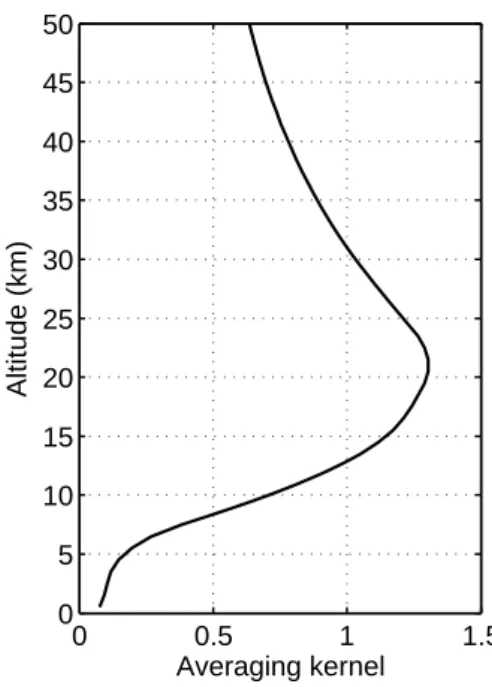
In this Section, we examine the sensitivity of the ground-based UV-visible twilight measurements to the vertical distri-bution of ozone in the troposphere and stratosphere through the use of the averaging kernels. These parameters are par-ticularly appropriate for that purpose since they describe the sensitivity of the slant column, i.e. the depth of the absorp-tion features in the measured spectra, to variaabsorp-tions of trace gas concentration at a given altitude. According to Eskes and Boersma (2003), the averaging kernel of layer l can be approximated by the ratio of the box-airmass factor of layer
l (AMFl)and the total air-mass factor (AMFtot)calculated from the ozone profile:
Al=AMFl/AMFtot
A typical example of such averaging kernels corresponding to 90◦ SZA at 45◦N in June is shown in Fig. 1. It has been computed using the UVSPEC/DISORT RTM (Mayer and Kylling, 2005) initialized with O3, pressure, and temper-ature profiles from the TOMS TV8 climatology (McPeters et al., 2007). Since the mean scattering layer is located around 14 km altitude, the sensitivity of zenith sky twilight measure-ments to tropospheric ozone is limited, with averaging ker-nel value smaller than 0.5 below 8 km, and increases in the
0 0.5 1 1.5 0 5 10 15 20 25 30 35 40 45 50 Averaging kernel Altitude (km)
Fig. 1. Column averaging kernel (left plot) computed for 90◦SZA in zenith-sky geometry using the ozone and temperature profiles
corresponding to 45◦N/325 DU in June extracted from the TOMS
V8 zonal mean climatology. The wavelength is fixed to 500 nm.
stratosphere where averaging kernel value is larger than 1 between 14–30 km altitude. So the twilight zenith-sky UV-vis total column ozone measurements are strongly weighted by the contribution of the stratosphere and therefore show very limited sensitivity to the uncertainties on parameters af-fecting tropospheric ozone like e.g. Mie scattering in a cloud layer. However, these measurements are sensitive to the tro-pospheric ozone column used for the AMF calculation which acts as a ghost column in the total column retrieval.
2.3 Recommended NDACC settings
So far, NDACC UV-visible groups commonly used their own DOAS settings and O3AMFs calculated with different RTMs and sets of ozone, pressure and temperature profiles, with or without latitudinal and seasonal variations. Differences be-tween AMFs are causing the largest discrepancies bebe-tween the NDACC O3data sets. The objective of the recommen-dations formulated by the NDACC UV-visible WG is thus to reduce these discrepancies through the use of standardized DOAS settings and O3AMF look-up tables (LUTs) that ac-count for the latitudinal and seasonal dependencies of the O3 vertical profile.
2.3.1 DOAS settings
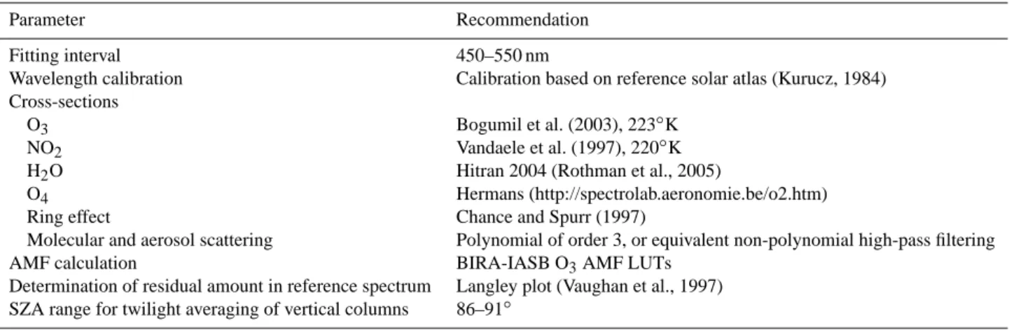
The NDACC recommendations for the ozone DOAS re-trieval are summarized in Table 1. Optimizing rere-trieval set-tings for total ozone in the visible Chappuis bands requires
Table 1. Settings recommended for the UV-visible retrieval of O3vertical columns.
Parameter Recommendation
Fitting interval 450–550 nm
Wavelength calibration Calibration based on reference solar atlas (Kurucz, 1984)
Cross-sections
O3 Bogumil et al. (2003), 223◦K
NO2 Vandaele et al. (1997), 220◦K
H2O Hitran 2004 (Rothman et al., 2005)
O4 Hermans (http://spectrolab.aeronomie.be/o2.htm)
Ring effect Chance and Spurr (1997)
Molecular and aerosol scattering Polynomial of order 3, or equivalent non-polynomial high-pass filtering
AMF calculation BIRA-IASB O3AMF LUTs
Determination of residual amount in reference spectrum Langley plot (Vaughan et al., 1997)
SZA range for twilight averaging of vertical columns 86–91◦
consideration on how the differential ozone signal can be ex-tracted with maximum sensitivity, while minimizing spectral interferences with other absorbers, which are, in the present spectral range, water vapor and the collision pair O2-O2. From sensitivity studies conducted on simulated spectra and actual measurements, it was found that ozone fitting uncer-tainties are minimized using the 450–550 nm spectral inter-val, which was therefore selected as a baseline for ozone re-trieval in the Chappuis bands. As an illustration, a typical example of fit result is displayed in Fig. 2. This was obtained in ScoresbySund, Greenland, on 16 July 2008, at 88.0◦SZA and 00:59 UT time. The retrieved contributions from O3, NO2, H2O, O4and Ring effect are shown separately. Given the importance of wavelength registration for DOAS evalua-tions in general, the recommendation is that measured spec-tra are aligned with the highest accuracy. This can be ob-tained by correlating measured spectra with a reference so-lar spectrum such as those of Kurucz (1984) or Chance and Spurr (1997), using least-squares techniques as implemented e.g. in the Windoas software suite (Fayt and Van Roozen-dael, 2009) or in the SAOZ analysis algorithm (Pommereau and Piquard, 1994). Different data sets of ozone absorption cross-sections are available from the literature. Comparison studies (e.g. Orphal, 2003) showed that differences of up to 4 percent can occur in the region of the Chappuis bands, and even more in the Huggins bands. Therefore the recom-mendation is the use of a common ozone cross-sections data set to avoid systematic differences. From test evaluations, that of Bogumil et al. (2003) is recommended since it gives the smallest variance in the residuals as well as good con-sistency with the ozone retrieval in the UV Huggins bands. Recommendations for laboratory cross section data sets of other species interfering in the 450–550 nm range are pro-vided in Table 1. Vandaele et al. (1997) at 220◦K is generally used for stratospheric NO2retrievals and therefore adequate for NO2removal in the O3fitting range. For correction of
2 1 0 -1 Ozone 1.0 0.5 0.0 -0.5 -1.0 NO2 1.0 0.5 0.0 -0.5 O4 measured fitted -0.4 0.0 0.4 H2O -0.2 0.0 0.2 Ring -0.5 0.0 0.5 550 540 530 520 510 500 490 480 470 460 450 Wavelength (nm) Residuals
Differential optical density (%)
Fig. 2. Typical example of ozone differential slant column fit
re-sult, obtained in ScoresbySund, Greenland, on 16 July 2008. The
spectrum was recorded at 00:59 UT and 88.0◦ SZA. The
succes-sive subplots display the respective contributions from O3, NO2,
O4, H2O and the Ring to the measured and simulated differential
optical density. Fitting residuals are shown at the bottom.
the Ring effect filling-in solar Fraunhofer lines, the approach published in Chance and Spurr (1997) is recommended. One should note that the ozone differential absorption features
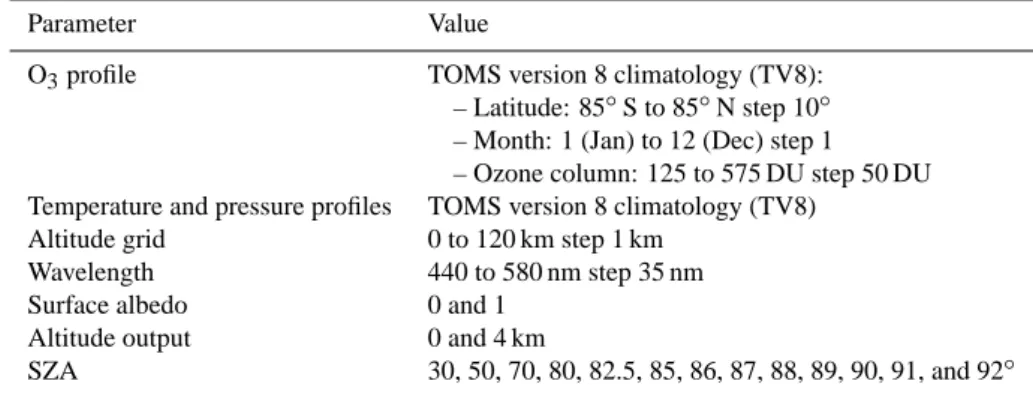
Table 2. Parameters used to initialize the UVSPEC/DISORT RTM for the calculation of the O3AMF LUTs.
Parameter Value
O3profile TOMS version 8 climatology (TV8):
– Latitude: 85◦S to 85◦N step 10◦ – Month: 1 (Jan) to 12 (Dec) step 1 – Ozone column: 125 to 575 DU step 50 DU
Temperature and pressure profiles TOMS version 8 climatology (TV8)
Altitude grid 0 to 120 km step 1 km
Wavelength 440 to 580 nm step 35 nm
Surface albedo 0 and 1
Altitude output 0 and 4 km
SZA 30, 50, 70, 80, 82.5, 85, 86, 87, 88, 89, 90, 91, and 92◦
are broad enough in the Chappuis bands to ensure that their filling-in by the Ring effect is quite small. However, due to its impact on the Fraunhofer lines, the Ring effect can-not be neglected. Finally, as already mentioned, the NDACC recommendation for twilight reporting is to average all re-trieved ozone vertical columns between 86◦ and 91◦ SZA. This range minimizes errors due to slant column fitting and AMF calculation (see Sect. 3) and provides stratospheric ozone measurements with limited sensitivity to tropospheric ozone and clouds.
2.3.2 O3AMFs
Description
Look-up tables (LUTs) of O3AMFs have been developed at the Belgian Institute for Space Aeronomy (BIRA-IASB) in support of the NDACC UV-visible WG. These are based on the TOMS version 8 (TV8) ozone and temperature profile climatology. TV8 is similar to the climatology of McPeters et al. (2007), i.e. a monthly mean climatology for 10◦latitude bands between 90◦S and 90◦N and covering altitudes from 0 to 60 km, with in addition a total O3column dependence (225–325 Dobson Unit (DU) in the tropics, 225–575 DU at mid-latitudes, and 125–575 DU at high-latitudes, with for all cases a 50 DU step). A total ozone column classification al-lows reproducing the short-term variations of the ozone pro-file. TV8 was built by combining profile data from SAGE II (Stratospheric Aerosol and Gas Experiment II), MLS (Mi-crowave Limb Sounder), and ozonesondes. This climatology has been widely utilized for the retrieval of global total ozone fields from recent US and European UV-visible nadir satellite sounders (e.g., Bhartia et al., 2004; Coldewey-Egbers et al., 2005; Eskes et al., 2005; Weber et al., 2005; Van Roozendael et al., 2006; Lamsal et al., 2007).
The O3AMF LUTs are calculated for the eighteen TV8 zonal bands using the UVSPEC/DISORT RTM which is based on the Discrete Ordinate Method and includes a treat-ment of the multiple scattering in a pseudo-spherical
geome-try. The model has been validated through several intercom-parison exercises (e.g., Hendrick et al., 2006; Wagner et al., 2007). Parameter values used to initialize UVSPEC/DISORT for the calculation of the AMF LUTs are summarized in Table 2. Since the TV8 climatology is limited to the 0– 60 km altitude range, the O3, temperature, and pressure pro-files are complemented above 60 km by the AFGL Standard Atmosphere for matching with the altitude grid chosen in UVSPEC/DISORT for the present study, which is 0–90 km. The surface albedo and altitude output values (varying from 0 to 1 and 0 to 4 km, respectively) allow covering all NDACC stations. Regarding the aerosol settings, an extinction profile corresponding to a background aerosol loading has been se-lected from the aerosol model of Shettle (1989) included in UVSPEC/DISORT. The present O3AMF LUTs are thus not suitable in case of large volcanic eruption such as that of the Mount Pinatubo in 1991.
The calculated LUTs depend on the following set of pa-rameters: latitude, day of year, O3 column, wavelength, SZA, surface albedo, and altitude. An interpolation routine has been designed for extracting appropriately parameter-ized O3 AMFs for the various NDACC stations. A global monthly mean climatology of the surface albedo derived from satellite data at 494 nm (Koelemeijer et al., 2003) is coupled to the interpolation routine, so the latter can be ini-tialized with realistic albedo values in a transparent way. The interpolation routine, O3 AMF LUTs, albedo clima-tology as well as DOAS settings are publicly available at http://uv-vis.aeronomie.be/groundbased.
Comparison to SAOZ O3AMFs
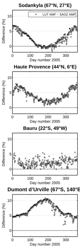
So far, SAOZ retrievals made use of constant AMFs cal-culated at the latitude of each station from mean SAGE II, POAM and SAOZ balloon profiles in the summer (Sarkissian et al., 1995). For illustrating the impact of using the new O3 AMF LUTs, time-series of AMFs have been extracted from the LUTs for one year of data at four SAOZ stations of the NDACC network: Sodankyla (67◦N, 27◦E), Observatoire
de Haute Provence (44◦N, 6◦E), Bauru (22◦S, 46◦W), and Dumont d’Urville (67◦S, 140◦E). The wavelength is fixed to 500 nm, the surface albedo to 0.2, and the station alti-tude to 0 km. The O3column values needed to properly ex-tract AMFs from the LUTs have been taken from the data files available on the NDACC database for year 2005. Com-parisons between LUT and SAOZ annual mean AMFs are shown in Fig. 3. As expected, the difference displays a strong seasonality. At mid- and high-latitudes, the largest differ-ence is seen in the winter with LUT AMFs larger than that of SAOZ by up to 8 %. In the summer, the difference is within the 0–2 % range in Sodankyla and OHP. At Dumont d’Urville (polar circle in the Southern Hemisphere), the LUT AMFs are larger than that of SAOZ by 11 % in the summer and 5 % in the winter. In the tropics, they are systematically larger by 2 % on average with no seasonality in the differ-ence, however the differences are noisier compared to other latitudes. This larger noise can be explained by the variabil-ity of the ozone profile shape above the Tropical Tropopause Layer (TTL) at altitudes from 20 to 30 km where the mea-surement sensitivity is largest (see Fig. 1), which therefore means a more significant impact on the AMF. As an exam-ple, the AMF in January in Bauru varies from 16.5 to 17.0, that is by 3 %, when using ozone profiles extracted from the TV8 climatology for typical total column values of 244 and 278 DU. Thus, small changes in total ozone of about 50 DU on a few days time scale, as frequently observed in Bauru, re-sult in significant changes in the AMF. For comparison, the AMF at 65◦N in April corresponding to total column val-ues of 332 and 417 DU (typical valval-ues around the mean total ozone column value at Sodankyla) is varying from 16.8 to 16.9, respectively, which corresponds to a change of 0.5 % only. This explains the smaller short-term variability in the AMF at mid- and high-latitudes.
3 Error budget
The error budget of the measurements is obtained by consid-ering error sources affecting the determination of the differ-ential slant column densities (DSCD), the residual amount in the reference spectrum (RCD), and the air mass factor (AMF).
3.1 DOAS analysis
Errors associated to the least-squares fit are due to detector noise, instrumental imperfections (small wavelength scale and resolution changes, etaloning and non-linearities of the detector, stray-light, polarisation effects, ...) as well as er-rors or unknowns in the signal modelling (Ring effect, un-known absorbers, wavelength dependence of the AMF, etc). To some extent, such errors are pseudo-random in nature and, as such, can be estimated statistically from the least-squares fit procedure. Fitting errors derived from the least-squares
0 100 200 300 0 5 10 Day number 2005 Difference (%) Sodankyla (67°N, 27°E)
LUT AMF − SAOZ AMF
0 100 200 300 0 5 10 Day number 2005 Difference (%)
Dumont d’Urville (67°S, 140°E)
0 100 200 300 0 5 10 Day number 2005 Difference (%)
Haute Provence (44°N, 6°E)
0 100 200 300 0 5 10 Day number 2005 Difference (%) Bauru (22°S, 49°W)
Fig. 3. Relative differences between LUT and SAOZ O3 AMFs
at 90◦SZA for the year 2005 at Sodankyla (67◦N, 27◦E),
Haute Provence (44◦N, 6◦E), Bauru (22◦S, 49◦W), and
Du-mont d’Urville (67◦S, 140◦E). The SAOZ tropical, high- and
mid-latitude O3AMF values at 90◦SZA are 16.20, 16.22, and 16.52,
Table 3. List of O3profile measurements used for testing the validity of the TV8 climatology for O3AMF calculations. The last column
is the mean relative difference (and the corresponding 1σ standard deviation) between O3AMF86−91◦SZA extracted from the LUTs and
calculated using the O3profiles measured at the different NDACC stations (see Fig. 4).
Station Instrument Time period Number Mean O3AMF86−91◦SZA
of profiles difference (%)
Ny- ˚Alesund (79◦N, 12◦E) O3sonde 01/2004–12/2006 218 −0.3 ± 1.3
Andoya (69◦N, 16◦E) Lidar 01/2004–12/2006 122 −1.7 ± 1.1
OHP (44◦N, 6◦E) O3sonde 01/2003–12/2006 113 −1.1 ± 1.3
Lidar 01/2004–12/2006 377 −1.2 ± 0.7
Iza˜na (28◦N, 16◦W) O3sonde 01/2004–12/2006 218 0.5 ± 1.7
Reunion Island (21◦S, 55◦E) O3sonde 01/2000–12/2002 59 −0.8 ± 1.8
Lauder (45◦S, 170◦E) O3sonde 01/2004–12/2006 139 −1.3 ± 0.9
Lidar 01/2004–12/2006 208 −1.4 ± 0.7
Dumont d’Urville (67◦S, 140◦E) O3sonde 07/2002–12/2006 116 0.4 ± 2.0
analysis typically give small uncertainties of the order 5 DU for O3DSCDs. However, results from intercomparisons ex-ercises (e.g. Van Roozendael et al., 1998; Vandaele et al., 2005; Roscoe et al., 2010) show that state-of-the-art instru-ments hardly agree to better than a few percents, even using standardised analysis procedures, which indicates that the ac-tual accuracy on the DSCDs is limited by uncontrolled in-strumental and/or analysis factors. Based on experience and results from intercomparison campaigns, we quote an uncer-tainty of the order of 3 % for the O3DSCD. This error adds up to systematic uncertainties on ozone absorption cross sec-tions in the Chappuis bands and on their (very small) temper-ature dependence which is of the order of 3 % in our spectral range (Orphal, 2003).
The accuracy on the determination of residual amount in the reference spectrum (RCD) is limited by the method used to derive the vertical column at the time of the reference spec-trum acquisition. Here we use a Langley-plot approach. The contribution from this error source to the total error budget is small, of the order of 1 %.
3.2 AMF LUTs
A potential source of uncertainty in our O3 AMF calcu-lation is related to the use of the TV8 O3 profile clima-tology, originally designed for nadir backscatter measure-ments from space. In order to test the validity of this cli-matology in the present context, O3 AMFs extracted from the LUTs have been compared to calculations performed using O3 profiles measured with ozonesondes and/or lidar observations at several NDACC stations representative of a wide range of conditions (tropics, mid- and high-latitudes). The stations and instruments used are listed in Table 3 and the data have been downloaded from the NDACC database (http://www.ndacc.org). In case of lidar, profiles have been complemented below their lower altitude limit by the TV8 climatology. Pressure and temperature profiles are taken
J F M A M J J A S O N D −5 0 5 Relative difference (%) OHP (44°N, 5.5°E) LUT − O3 sonde J F M A M J J A S O N D −5 0 5 Relative difference (%) LAU (45°S, 170°E) LUT − O3 sonde J F M A M J J A S O N D −5 0 5 Relative difference (%) NYA (79°N, 12°E) LUT − O3 sonde J F M A M J J A S O N D −5 0 5 IZA (28°N, 16°W) LUT − O3 sonde J F M A M J J A S O N D −5 0 5 REU (21°S, 55°E) LUT − O3 sonde J F M A M J J A S O N D −5 0 5 DDU (67°S, 140°E) LUT − O3 sonde J F M A M J J A S O N D −5 0 5 LAU (45°S, 170°E) LUT − O3 LIDAR J F M A M J J A S O N D −5 0 5 OHP (44°N, 5.5°E) LUT − O3 LIDAR J F M A M J J A S O N D −5 0 5 AND (69°N, 16°E) LUT − O3 LIDAR
Fig. 4. Relative difference between O3AMF86−91◦SZAextracted
from the LUTs and calculated using the O3profiles measured at the
following NDACC stations: Ny- ˚Alesund (NYA), Andoya (AND),
Observatoire de Haute Provence (OHP), Iza˜na (IZA), Reunion Is-land (REU), Lauder (LAU), and Dumont d’Urville (DDU). Filled grey squares: daily relative differences, black solid lines: yearly mean relative difference, and black dashed lines: 1σ standard devi-ation (see Table 3 for corresponding values).
from the AFGL Standard Atmosphere when not available in the lidar data files. The aerosol extinction profile is the same as the one used for the calculation of the LUTs (see first sub-section of Sect. 2.3.2). Other settings required for initializ-ing the UVSPEC/DISORT RTM are identical to those fixed
for the extraction of the O3 AMFs from the LUTs (wave-length: 500 nm, surface albedo: 0.2, station altitude: 0 km). O3 AMFs are calculated for between 86 and 91◦ SZA by 1◦ SZA step using the measured O3 profiles and compared to those extracted from the LUTs for the same SZA range. Figure 4 depicts the seasonal variation of the difference be-tween LUT AMFs and those calculated from sonde or li-dar measurements between 86 and 91◦SZA (called hereafter AMF86−91◦SZA). The yearly mean differences are reported in
Table 3. On average, the largest mean relative differences be-tween O3AMF86−91◦SZAextracted from the LUTs and those
calculated with the measured O3profiles are obtained with li-dar. However, these relative differences show smaller season-ality and less noise than those derived from the sondes, espe-cially at high latitude at Ny- ˚Alesund and Dumont D’Urville and in the tropics at Iza˜na and Reunion Island. These sig-nificant residual seasonalities could be related to the zonal dependence of the tropospheric ozone seasonality not imple-mented in the TV8 climatology and displaying a maximum in the summer at the Northern Hemisphere and in spring at the southern tropics (see Figs. 15 and 16), and to systematic errors in the TV8 in the winter at high latitude at low sun where SAGE II data are no more available. The larger noise with the sondes might come from their precision limited to 5 %. Nevertheless, since the mean relative difference for the nine comparison cases considered here is −1 ± 1.3 %, these results show that the TV8 climatology reproduces well on average the mean O3 profiles latitudinal and seasonal vari-ations, so that sufficiently accurate O3AMFs can be calcu-lated.
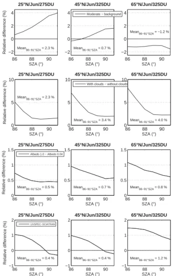
The choice of the aerosol extinction profile is also a source of uncertainty in our O3 AMF calculations. The UVSPEC/DISORT RTM includes the aerosol climatology of Shettle (1989), which consists of a set of extinction profiles corresponding to different volcanic conditions (background, moderate, high, and extreme). For the present study, we have selected the aerosol extinction profile corresponding to background conditions, with a surface visibility of 40 km (called hereafter the standard settings). In order to give an upper limit of the uncertainty related to the choice of the aerosol settings, O3 AMFs corresponding to moderate vol-canic conditions have been calculated. The O3profiles are selected from the TV8 climatology for the following con-ditions: 25◦N/275 DU, 45◦N/325 DU, and 65◦N/325 DU in June. Figure 5 (upper panels) shows the comparison of O3 AMFs calculated with standard and moderate volcanic aerosol settings. The relative difference is smaller than 2 % except at SZA larger than 87◦ in the tropics where the O
3 AMFs corresponding to moderate volcanic conditions are larger than the standard ones by up to 4 %. However, the mean relative difference in the 86–91◦SZA range for the three selected O3profiles is 0.6 %. Similar comparison re-sults are obtained for winter O3profiles.
Clouds are not accounted for in our O3AMF calculations but their impact has been investigated using the water clouds
86 88 90 −2 0 2 4 SZA (°) Relative difference (%) 25°N/Jun/275DU Mean86−91°SZA = 2.3 % 86 88 90 −2 0 2 4 SZA (°) 45°N/Jun/325DU Mean86−91°SZA = 0.7 % Moderate − background 86 88 90 −2 0 2 4 SZA (°) 65°N/Jun/325DU Mean86−91°SZA = −1.2 % 86 88 90 0 5 10 SZA (°) Relative difference (%) 25°N/Jun/275DU Mean86−91°SZA = 2.3 % 86 88 90 0 5 10 SZA (°) 45°N/Jun/325DU Mean86−91°SZA = 3.4 %
With clouds − without clouds
86 88 90 0 5 10 SZA (°) 65°N/Jun/325DU Mean86−91°SZA = 4.0 % 86 88 90 −1 0 1 2 SZA (°) Relative difference (%) 25°N/Jun/275DU Mean86−91°SZA = 0.4 % UVSPEC−SCIATRAN 86 88 90 −1 0 1 2 SZA (°) Mean86−91°SZA = 0.4 % 45°N/Jun/325DU 86 88 90 −1 0 1 2 SZA (°) Mean86−91°SZA = 1.2 % 65°N/Jun/325DU 86 88 90 0 0.5 1 1.5 SZA (°) Relative difference (%) 25°N/Jun/275DU Mean86−91°SZA = 0.5 % Albedo 1.0 − Albedo 0.04 86 88 90 0 0.5 1 1.5 SZA (°) Mean86−91°SZA = 0.7 % 45°N/Jun/325DU 86 88 90 0 0.5 1 1.5 SZA (°) Mean86−91°SZA = 0.8 % 65°N/Jun/325DU
Fig. 5. From top to bottom, comparison of O3AMFs calculated
us-ing standard and moderate volcanic aerosol settus-ings, with and with-out the presence of clouds, with surface albedo fixed to 1.0 and 0.04, and with UVSPEC and SCIATRAN RTMs. The mean
rela-tive difference calculated in the 86–91◦SZA range appears on each
plot. In case of the aerosols sensitivity test, the overall mean relative
difference over the 86–91◦SZA range is of 0.6 % while it reaches
3.3 %, 0.7 %, and 0.7 % for the test on clouds, surface albedo, and
RTMs, respectively. The O3profiles selected from the TV8
clima-tology for the present comparison correspond to the following
con-ditions: 25◦N/275 DU (left plots), 45◦N/325 DU (middle plots),
and 65◦N/325 DU (right plots) in June. The wavelength, surface
albedo, and altitude are fixed to 500 nm (541 nm for test on RTMs),
0.2, and 0 km, respectively. O3AMF are mostly impacted by the
presence of clouds (stratus layer in the present case), reducing the
AMF by 3.4 % on average in the 86–91◦SZA range at mid-latitude.
model included in UVSPEC/DISORT. The way to initialize this model is to specify the vertical profile of liquid water content and effective droplet radius. The microphysical prop-erties of water clouds are then converted to optical proper-ties according to the Hu and Stamnes (1993) parameteriza-tion. O3 AMFs are calculated for cloudy and non-cloudy
conditions for the same TV8 climatology O3 profiles as above (25◦N/275 DU, 45◦N/325 DU, and 65◦N/325 DU in June). For cloudy conditions, the cloud model parameters values are fixed as follows: water content: 0.3 g m−3, ef-fective droplet radius: 5 µm, cloud layer thickness and alti-tude: 1 km between 1 and 2 km. Since these parameters val-ues correspond to a rather large stratus cloud (Shettle, 1989), the present sensitivity test gives an upper limit of the impact of clouds on O3 AMFs. A comparison of O3 AMFs calcu-lated for cloudy and non-cloudy conditions is presented in Fig. 5 (2nd line panel). Cloudy AMFs are systematically larger than non-cloudy AMFs by about 5–8 % at 86◦SZA and 2 % at 91◦SZA. The mean relative difference in the 86– 91◦SZA range for the three selected O3profiles is of 3.3 %. Similar comparison results are obtained for winter O3 pro-files. The small impact of clouds on zenith-sky ozone UV-vis measurements at twilight is due to the fact that the mean scattering layer is generally located at higher altitude than that of the clouds. However, there are two exceptions: in the tropics where thunderstorms accompanied by heavy rainfall can reach 15–16 km, and at high latitude in the winter where Polar Stratospheric Clouds (PSC) are sometimes present, dis-turbing the ozone measurements. These episodes are easily removed from the ground-based data series by detecting the large enhancements of 70 % or more of the absorption by O4 and H2O in the tropics in the presence of thick clouds and rainfall, and by the use of a color index (ratio between irra-diances at 550 and 350 nm) in case of PSC (Sarkissian et al., 1991).
Another source of uncertainty we have tested is the im-pact of surface albedo. O3AMFs corresponding to the same three TV8 climatology O3profiles as above have been calcu-lated using the UVSPEC/DISORT RTM with albedo fixed to 0.04 (ice free sea) and 1 (fresh snow, sea ice or thunderstorm anvils). Results are shown in Fig. 5 (3rd line panels). Within the 86–91◦SZA range, the impact of surface albedo is rather low with a mean relative difference between albedo 1.0 and 0.04 cases of 0.7 % for the three selected O3profiles.
A last source of uncertainty is the impact of the RTM used for AMF calculations. Although previous studies (e.g., Hendrick et al., 2006; Wagner et al., 2007) have demon-strated that, for AMF calculation, the UVSPEC/DISORT model shows very good consistency with others RTMs, a verification exercise has been carried out to firmly as-sess the reliability of the present O3 AMF calculations. It consists in comparing O3 AMFs calculated using the UVSPEC/DISORT and SCIATRAN v2.2 RTMs initialized in the same way. SCIATRAN is based on the Combining Differential-Integral approach using the Picard-Iterative ap-proximation (CDIPI) and includes a treatment of multiple scattering in full or pseudo-spherical geometry (Rozanov et al., 2005). The following settings have been used for the present exercise: pseudo-spherical geometry, TV8 O3 pro-file climatology, AFGL Standard Atmosphere pressure and temperature profiles, TV8 atmosphere layering (Umkehr
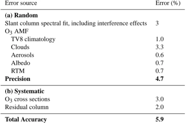
lay-Table 4. Error budget of zenith-sky total O3columns measurements
in the visible (%).
Error source Error (%)
(a) Random
Slant column spectral fit, including interference effects 3 O3AMF TV8 climatology 1.0 Clouds 3.3 Aerosols 0.6 Albedo 0.7 RTM 0.7 Precision 4.7 (b) Systematic O3cross sections 3.0 Residual column 2.0 Total Accuracy 5.9
ers), wavelength: 541 nm, surface albedo: 0, station altitude: 0 km. Regarding the O3 profile, the following cases have been considered: polar latitude in January and June (65◦N and S with a total column of 325 DU, mid-latitude in Jan-uary and June (45◦N and S, 325 DU), and tropics in Jan-uary and June (25◦N and S, 275 DU). The results for the Northern Hemisphere in June are shown in Fig. 5 (bottom panels). Both models are in excellent agreement with rela-tive differences smaller than 1.5 %. Within the 86-91◦SZA range, the mean relative difference is 0.7 %. Since similar consistency is found in January and in the Southern Hemi-sphere, this comparison demonstrates the reliability of the UVSPEC/DISORT RTM for O3AMF calculation.
The overall error budget of twilight zenith-sky visible total O3total columns measurements is summarized in Table 4. The precision by adding quadratic random errors is 4.7 % to which the largest contribution is coming from the AMF and from the error on the slant column estimated to be 3 % at twilight, including the impact of unknown instrumental and systematic misfit effects. The total accuracy, important for comparison with other instruments, is 5.9 %.
4 Application of the recommended settings to the
NDACC/SAOZ network
The French led SAOZ (Syst`eme d’Analyse par Obser-vation Z´enithale) network contributes significantly to the NDACC/UV-visible network with about 20 instruments cov-ering a wide range of latitudes in both hemispheres. The SAOZ instrument is a broad-band (300–600 nm), medium resolution (1 nm) diode-array spectrometer that observes sunlight scattered at zenith sky (Pommereau and Goutail, 1988; Sarkissian et al., 1997). Absorption spectra are
recorded hourly at SZA smaller than 85◦ and every 5 min during twilight up to 94◦SZA. The full SAOZ data set has been reprocessed in a version V2 using the NDACC recom-mendations. The previous version, called V1, was using con-stant AMFs specific to each station (see second subsection of Sect. 2.3.2) and, regarding the DOAS settings, differs from V2 on the Ring and ozone cross-sections and the wavelength fitting window. The impact of the changes of these three pa-rameters is discussed below.
i. Ring cross-sections. The SAOZ V1 Ring cross-sections were derived from a high-resolution differential ref-erence spectrum. The change for Chance and Spurr (1997) procedure leads to an insignificant increase by 0.1 % ± 0.01 % of the ozone slant column.
ii. Ozone cross-sections. SAOZ V1 was using a combi-nation of two laboratory data sets, those of the GOME flight model (FM) at 202 K between 330 and 514.5 nm (Burrows et al., 1999) and of Brion et al. (1998) be-tween 514.5 and 650 nm, both normalized on Anderson and Mauersberger (1992) absolute cross-sections mea-sured at six wavelengths thought to be the most pre-cise available (GOME FM cross-sections multiplied by 1.029 and Brion et al. by 1.021). The change for Bogu-mil et al. (2003), leads to a decrease of the ozone slant column by 0.8 % ± 0.01 %.
iii. Ozone fitting window. For taking the advantage of the 8 ozone cross-sections differential features available in the Chappuis bands, the SAOZ V1 spectral range ex-tended from 450–617 nm, with the exception of the 580–602 nm ignored because of the presence of water vapor absorption bands at around 590 nm particularly intense in the warm tropics. The change for the 450– 550 nm spectral range in the SAOZ V2 leads to an in-crease of ozone slant column by 1.6 % ± 0.05 %. How-ever, the cause of this larger ozone is not the spectral fitting but the decrease of slant column at increasing wavelength because of the lower altitude of the mean scattering level of sunlight at twilight. After conversion into vertical column using SAOZ AMFs calculated at the center of the windows, of 16.41 at 500 nm instead of 16.22 at 540 nm, the change in vertical column is only 0.2 % ± 0.05 %.
Overall, the change between V1 and V2 after applying the NDACC UV-Vis working group recommendations for DOAS settings is a decrease of ozone vertical column at twilight by 0.5 %, which is not significant.
4.1 Comparison to Dobson and Brewer
In order to assess the newly derived SAOZ V2 data set, com-parisons were performed using two reference ground-based UV ozone spectrophotometers collocated with SAOZ instru-ments: a Dobson at OHP and a Brewer at Sodankyla.
4.1.1 Dobson at OHP
The instrument is the Dobson #085 operating at this station since 1983. A comparison of the total ozone columns mea-sured by the Dobson and SAOZ (V2 retrieval) spectrometers is presented in Fig. 6. The difference Dobson-SAOZ showed in the past a systematic seasonal variation with a summer maximum, but of amplitude larger than that expected from the temperature dependence of the UV cross-sections only. According to Van Roozendael et al. (1998), it can also orig-inate in the seasonal AMF variation not taken into account in the operational SAOZ retrievals. Consistent with this, the replacement of the SAOZ constant AMF by AMF LUTs re-duces the amplitude of the seasonal Dobson-SAOZ differ-ence from 6.9 % to 3.2 % (see Fig. 7). After applying this cor-rection, the correlation of the Dobson-SAOZ V2 difference with ECMWF temperature indicates a dependence of the difference Dobson-SAOZ V2 of 0.25 ± 0.02 %/◦C at 50 hPa and 0.20 ± 0.01 %/◦C at 30 hPa, or 0.18 %/◦C at 30 hPa us-ing the NCEP temperature. The 30 hPa temperature is more relevant at OHP since it corresponds better to the altitude of the maximum of ozone concentration. After correction for the temperature dependence at 30 hPa, the amplitude of the seasonal variation decreases to 1.2 % with a yearly mean bias of −1.1 ± 3.7 %. This 0.18 %/◦C temperature depen-dence is significantly larger than the 0.13 %/◦C calculated by Komhyr et al. (1993) for the Dobson AD pair from the Bass and Paur ozone absorption cross sections (Paur and Bass, 1985), the 0.11 %/◦C proposed by Van Roozendael et al. (1998) from Malicet et al. (1995) cross sections, or even the 0.02 %/◦C of Burrows et al. (1999) as summarized by Scarnato et al. (2009). However, it is very similar to the 0.21 %/◦C found with TOMS and OMI-TOMS.
Aside from a possible underestimation of the temperature dependence of the absorption cross sections at low tempera-ture, another possible additional contribution to the seasonal variation of the difference with SAOZ could be the influence of tropospheric ozone to which, in contrast to Dobson direct sun observations, SAOZ is less sensitive. As displayed later in Fig. 15, the tropospheric ozone column at OHP shows a systematic seasonality of about 15 DU amplitude with a sum-mer maximum, which might explain the remaining seasonal cycle of 1–1.5 % amplitude in the Dobson-SAOZ difference. Moreover, the Dobson instrument has internal stray light that produces an error with a SZA dependence, which is more pronounced at high ozone values. However, the magnitude of this effect is difficult to estimate, but it can also contribute to the residual seasonal cycle of the Dobson-SAOZ differ-ences.
In summary, the 3.2 % residual seasonal amplitude of the Dobson-SAOZ V2 difference at OHP can be partly explained by a known temperature dependence of the absorption cross-sections at Dobson wavelengths not taken into account in the Dobson retrievals and varying between 0.11–0.13 %/◦C according to laboratory measurements and 0.18 %/◦C in the
400
350
300
250
Total ozone (DU)
-10 -5 0 5 10 Dobson-SAOZ (%) 1993 1995 1997 1999 2001 2003 2005 2007 2009
Fig. 6. Comparison between Dobson (black line) and SAOZ V2
(grey line) total ozone columns at OHP (upper plot). The relative difference Dobson-SAOZ V2 appears on the lower plot (grey dots: daily; black lines: monthly mean). SAOZ data in 1992–1993 are removed because of the Mount Pinatubo eruption. The difference shows a systematic seasonal cycle, and small systematic offsets be-tween periods of several years as well as sporadic jumps on some months. Since they do not correlate with changes in the satellite-SAOZ difference at OHP they cannot be attributed to satellite-SAOZ.
present study, and by uncertainties in the ozone profile sea-sonal variation in the TV8 climatology, particularly in the troposphere. The mean 1 % low bias of the SAOZ com-pared to Dobson is within the uncertainties of absolute cross-sections used by both instruments.
4.1.2 Brewer MKII at Sodankyla
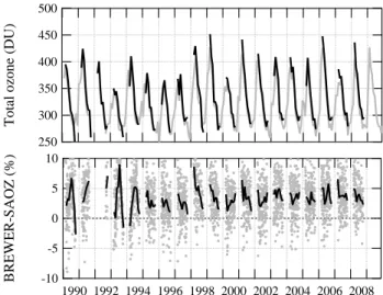
The Brewer and the SAOZ instruments in Sodankyla were al-ready compared in 1990–91 (Kyr¨o, 1993; Van Roozendael et al., 1998). The SAOZ showed a systematic bias varying from
−9±5 % if only Brewer measurements at SZA < 60◦ were considered and +2 % using all Brewer data. The seasonal cycle of the ratio between the Brewer and SAOZ measure-ments was highly correlated with the temperature at 50 hPa, but at a rate of 0.34 %/◦C, exceeding largely the 0.07 %/◦C Brewer temperature dependence derived by Kerr et al. (1988) from the ozone cross sections of Paur and Bass (1985). At that time, no explanation was found for this discrepancy but the SAOZ retrieval was the V1 version based on the use of a constant AMF derived from a mean winter ozone profile. Figure 8 shows the Brewer and SAOZ V2 series of ozone col-umn over Sodankyla since 1990 and the corresponding rela-tive difference. The winter Brewer zenith-sky observations are ignored since displaying large drops as well as the 1992 SAOZ data due to the large aerosols loading changes asso-ciated to the Mount Pinatubo eruption. Asides from these periods, the Brewer values are larger than those of SAOZ
-10 -5 0 5 10 Dobson - SAOZ (%)
JAN FEBMAR APR MAY JUN JUL AUG SEP OCT NOV DEC
Fig. 7. Seasonal variation of the Dobson-SAOZ relative difference
at OHP (dashed line: SAOZ V1, dotted line: SAOZ V2, solid line: Dobson corrected for temperature).
500 450 400 350 300 250
Total ozone (DU)
-10 -5 0 5 10 BREWER-SAOZ (%) 1990 1992 1994 1996 1998 2000 2002 2004 2006 2008
Fig. 8. Comparison between Brewer (black line) and SAOZ V2
(grey line) total ozone columns at Sodankyla. The relative dif-ference Brewer-SAOZ V2 appears on the lower plot (grey dots: daily; black lines: monthly mean). SAOZ data in 1992–1993 are removed because of the Pinatubo eruption. Because of the polar night, Brewer measurements are absent during the winter. Small systematic offsets sometimes also appear, e.g., after 1997 and 2001.
by 3–4 % on average, showing sometimes large deviations in October or March, i.e. at the beginning and the end of the winter. Figure 9 shows the average seasonal cycle of the dif-ference. The change from SAOZ V1 to SAOZ V2 decreases the amplitude of the seasonal cycle from 4 % to 2.4 %, pro-viding an explanation to Kyr¨o (1993) interrogation. The correlation with ECMWF temperature indicates a depen-dence of the Brewer-SAOZ difference of 0.06 ± 0.01 %/◦C at 50hPa and of 0.05 ± 0.01 %/◦C at 30 hPa, the first one being most relevant at this latitude. After correction for the temperature dependence at 50 hPa, the amplitude of the seasonal variation decreases to 1.4 % and the mean bias is 2.7 ± 3.4 %. The coefficient of 0.06 %/◦C is very consistent with the 0.07 %/◦C and 0.08 %/◦C estimated from Paur and
Bass (1985) cross-sections by Kerr et al. (1988) and Scarnato et al. (2009), respectively, but smaller than the 0.09 %/◦C of Kerr et al. (2002) from the same data but using differ-ent sets of temperature, or the 0.13 %/◦C derived by Scar-nato et al. (2009) from the Malicet et al. (1995) ozone cross-sections. However, Scarnato et al. (2009) have shown that these coefficients depend on the instrument, the tempera-ture range, and on the method of calculation from laboratory cross-sections. In addition, Savastiouk and McElroy (2010) have estimated that a change from Paur and Bass (1985) to Malicet et al. (1995) absorption cross-sections would make the Brewer data lower by 3 % on average, that is in full agree-ment with SAOZ V2.
In summary, the difference between Brewer and SAOZ in Sodankyla can be fully explained by a temperature depen-dence of 0.06 %/◦C and the 3 % mean bias between them by the uncertainty in the ozone absorption cross-sections used in the Brewer retrieval.
4.2 Comparison to satellite observations
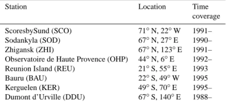
Six total ozone satellite data series are available since the be-ginning of the deployment of the SAOZ network in 1988: the TOMS V8 series from Nimbus-7, Meteor-3, and Earth Probe between 1989 and 2005, available from the NASA GSFC database (http://toms.gsfc.nasa.gov, Wellemeyer et al., 2004); the GOME-GDP4 observations from 1995 to 2003 for all stations and until present for the European sector after the failure of the onboard data recorder, avail-able from the operational ESA GDP4 level 2 (http://wdc. dlr.de/sensors.gome/gdp4/; Van Roozendael et al., 2006); the SCIAMACHY-TOSOMI columns since 2002, available from the ESA – KNMI TEMIS site (http://www.temis.nl/ protocols/o3col/overpass scia.html; Eskes et al., 2005), the SCIAMACHY off-line version 3 (OL3) retrievals available from the ftp site ftp-ops-dp.eo.esa.int, and the AURA OMI-TOMS and OMI-DOAS collection 3 retrievals since 2004 available from the NASA AVDC (http://avdc.gsfc.nasa.gov; Veefkind et al., 2006; Kroon et al., 2008). All the data used here are overpass total ozone columns above each station within a 300 km radius. Eight SAOZ stations, those show-ing the longest data time-series and continuous observations throughout the year, have been selected for the present com-parison (see Table 5): three in the Arctic (Scoresbysund, Zhi-gansk, and Sodankyla), one at northern mid-latitude (Obser-vatoire de Haute Provence), two at the southern tropics (Re-union Island and Bauru), one at the southern mid-latitude (Kerguelen) and one in the Antarctic (Dumont d’Urville). Because of the perturbation of the SAOZ zenith-sky total ozone measurements by the volcanic aerosols injected in the stratosphere by the eruption of Mount Pinatubo in 1991, the measurements performed between October 1991 and Octo-ber 1992 have been ignored.
-10 -5 0 5 10 Brewer-SAOZ (%) J F M A M J J A S O N D
Fig. 9. Seasonal variation of the Brewer-SAOZ relative differ-ence at Sodankyla (dashed line: SAOZ V1, dotted line: SAOZ V2, solid line: Brewer corrected for temperature).
Table 5. List of the SAOZ stations used in the study.
Station Location Time
coverage
ScoresbySund (SCO) 71◦N, 22◦W 1991–
Sodankyla (SOD) 67◦N, 27◦E 1990–
Zhigansk (ZHI) 67◦N, 123◦E 1991–
Observatoire de Haute Provence (OHP) 44◦N, 6◦E 1992–
Reunion Island (REU) 21◦S, 55◦E 1993
Bauru (BAU) 22◦S, 49◦W 1995
Kerguelen (KER) 49◦S, 70◦E 1995–
Dumont d’Urville (DDU) 67◦S, 140◦E 1988–
4.2.1 V2 versus V1 SAOZ data sets
As an example, monthly mean total ozone column and rel-ative difference satellite-SAOZ V2 at OHP since 1995 for TOMS and GOME-GDP4 (the two longest satellite records) are presented in Fig. 10. The difference shows a systematic seasonal variation with a summer maximum. The amplitude of the seasonal cycle of the difference is larger with TOMS (4.7 %) than with GOME-GDP4 (1.2 %).
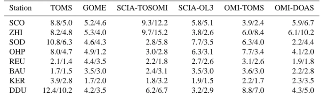
Figure 11 depicts the change between SAOZ V1 and V2 in the difference satellite-SAOZ at Sodankyla, OHP, Bauru and Dumont d’Urville. The use of V2 instead of V1 reduces the amplitude of the seasonal cycle of the difference with TOMS from 10.8 % to 6.3 % at Sodankyla and from 8.0 % to 4.7 % at OHP, and from 4.6 % to 4.3 % and 4.9 % to 1.2 % for the same stations with GOME-GDP4. The use of SAOZ V2 has a limited impact in Bauru (tropics), where the amplitude of the relative difference varies from 1.7 % to 1.5 % with TOMS and from 3.5 % to 3.0 % with GOME-GDP4, but decreases the mean total ozone by about 3 %. The same feature is found at Dumont d’Urville where the seasonal cycles is reduced only from 12.4 to 10.2 % and 4.2 to 3.5 % with TOMS and GOME, respectively, but the mean total ozone is decreased by 5 % with SAOZ V2.
Table 6 summarizes the change in the seasonal cycle of the satellite-SAOZ difference for all selected stations and satel-lites. The replacement of the SAOZ V1 by the V2 version
Table 6. Amplitude (%) of the seasonal cycle of the relative differences satellite – SAOZ (V1/V2). See Table 5 for the meaning of the
abbreviations of the stations.
Station TOMS GOME SCIA-TOSOMI SCIA-OL3 OMI-TOMS OMI-DOAS
SCO 8.8/5.0 5.2/4.6 9.3/12.2 5.8/5.1 3.9/2.4 5.9/6.7 ZHI 8.2/4.8 5.3/4.0 9.7/15.2 3.8/2.6 6.0/8.4 6.1/10.2 SOD 10.8/6.3 4.6/4.3 2.8/5.8 7.7/3.5 6.3/4.0 2.2/4.4 OHP 8.0/4.7 4.9/1.2 3.0/2.8 6.3/3.1 7.7/3.4 4.1/2.0 REU 2.1/1.4 4.4/3.5 2.2/1.8 2.7/2.6 3.1/2.6 1.9/1.8 BAU 1.7/1.5 3.5/3.0 2.4/3.1 3.5/3.0 3.6/3.0 2.2/2.8 KER 3.9/2.8 1.7/2.0 1.8/3.2 1.9/1.5 2.2/1.7 2.3/3.5 DDU 12.4/10.2 4.2/3.5 6.2/6.7 3.2/2.9 8.8/7.0 4.3/5.0 400 350 300 250 -10 -5 0 5 10 1993 1995 1997 1999 2001 2003 2005 2007 2009 1993 1995 1997 1999 2001 2003 2005 2007 2009
Total ozone (DU)
Sat.-SAOZ (%)
TOMS GOME
Fig. 10. Example of comparison between SAOZ V2 and satellite
overpass total ozone at OHP. Top: monthly mean total ozone (grey line: SAOZ; black line: satellite), bottom: satellite-SAOZ relative difference (grey dots: daily; black lines: monthly mean). Left: TOMS, right: GOME-GDP4.
reduces on average the amplitude of the seasonal cycle of dif-ferences with TOMS, GOME, SCIA-OL3, and OMI-TOMS although systematic seasonal cycles still remain, of partic-ularly large amplitude at high latitude. However, there are satellites for which the change from V1 to V2 increases the amplitude of the cycle, particularly SCIA-TOSOMI and OMI-DOAS at high latitude. This comes from larger uncer-tainties in some satellite retrievals at large SZA at the be-ginning and the end of the winter period, even if all satellite data have been uniformly limited to SZA < 84◦. The yearly mean AMF used in the SAOZ V1 retrieval is thus not the only parameter responsible for the seasonal cycle of the satellite-SAOZ and other parameters are implied. As already shown by Lambert et al. (1999), parameters displaying systematic seasonal cycles which could potentially affect the retrievals are: the temperature of the stratosphere and the SZA of satel-lite measurements, showing both a summer maximum, and the seasonal variation of the ozone column which presents a maximum in spring at mid- and high latitude.
-10 -5 0 5 10 -10 -5 0 5 10 -10 -5 0 5 10 -10 -5 0 5 10 J F M A M J J A S O N D -10 -5 0 5 10 -10 -5 0 5 10 -10 -5 0 5 10 -10 -5 0 5 10 J F M A M J J A S O N D Sat.-SAOZ (%)
TOMS SODANKYLA GOME
OHP
BAURU
DUMONT
Fig. 11. Seasonal variation of the satellite-SAOZ relative difference
(dashed lines: SAOZ V1, dotted lines: SAOZ V2). From top to bot-tom: Sodankyla, OHP, Bauru, and Dumont d’Urville. Left: TOMS, right: GOME-GDP4. The error bars correspond to the 1σ devia-tions, which increase during the winter, particularly at high latitude.
Table 7. Temperature dependence of satellite-SAOZ V2 relative
difference at 50 and 30 hPa (in %/◦C).
Satellite 50 hPa 30 hPa
TOMS + 0.21 ± 0.003 + 0.24 ± 0.003 GOME-GDP4 + 0.06 ± 0.004 + 0.08 ± 0.004 SCIA-TOSOMI + 0.09 ± 0.006 + 0.14 ± 0.006 SCIA-OL3 + 0.11 ± 0.004 + 0.12 ± 0.004 OMI-TOMS + 0.21 ± 0.004 + 0.16 ± 0.004 OMI-DOAS + 0.00 ± 0.005 + 0.00 ± 0.005
Table 8. SZA dependence of satellite-SAOZ V2 relative difference
at 50 hPa: b× SZA +c× SZA3.
Satellite b c(×10−6) TOMS +0.02 −1.7 GOME-GDP4 +0.06 −1.8 SCIA-TOSOMI −0.01 +16.2 SCIA-OL3 +0.00 +4.0 OMI-TOMS +0.00 +6.7 OMI-DOAS +0.02 +7.3
4.2.2 Stratospheric temperature, SZA, and ozone
column dependencies
The influence of these parameters has been investigated by correlating the satellite-SAOZ difference with daily ECMWF temperature at 50 hPa and 30 hPa, SZA at the location of the satellite measurements, and ozone total column. The correlation was performed on daily measurements from all stations together (sunrise-sunset average in case of SAOZ). For removing the systematic mean biases between the tions discussed in Sect. 4.2.3, the average bias of each sta-tion has been set to zero at 210 K and 50◦ SZA. As an ex-ample, Fig. 12 depicts the correlation between the difference between TOMS and SAOZ and SCIA-TOSOMI and SAOZ with temperature at 50 hPa on the left, and SZA on the right, after removing the satellite measurements at SZA > 84◦ where they are known as less reliable. Since not significant, the dependence on total ozone columns is not shown. The calculation involves more than 30 000 data points. These two satellites have been chosen here because showing the largest temperature (TOMS) and SZA (SCIA-TOSOMI) dependen-cies. TOMS displays a linear temperature dependence of 0.21 %/◦C resulting in a seasonal amplitude of more than 10 % amplitude in the Antarctic and a negligible SZA de-pendence of 0.01 %/◦SZA, which represents only 0.4 % of amplitude in seasonality. In contrast, SCIA-TOSOMI shows a temperature dependence of 0.08 %/◦C only, but a large and non-linear SZA dependence, approximated by a cubic law, of −0.01 %/◦SZA + 16.2 × 10⁻⁶%/◦SZA3, leading to a
sea--20 0 20 240 220 200 180 -20 0 20 80 60 40 20 0 DDU SCO SOD ZHI KER OHP REU BAU -20 0 20 240 220 200 180 -20 0 20 80 60 40 20 0 TOMS-SAOZ (%)
T dependency SZA dependency
SCIAtosomi-SAOZ (%)
T50hPa (°K) SZA satellites (°)
Fig. 12. Correlation between daily satellite-SAOZ difference and
ECMWF temperature at 50 hPa (left), and SZA of satellite measure-ments (right) for the height SAOZ stations altogether. Top: TOMS; Bottom: SCIA-TOSOMI.
sonal variation of total ozone of 9 % amplitude at high lati-tude. Such SZA dependence of a nadir-viewing satellite in-strument is coming from the increasing altitude of the sun-light scattering layer at increasing SZA, not properly taken into account in the retrieval. Note that a confusion between SZA and temperature in the correlations shown in Fig. 12 is not possible, since (1) the first is peaking at the solstice and the second in the mid-summer, and (2) the amplitude of the temperature variation is limited to 15◦C in the tropics, while that of SZA is varying by about 45◦.
The results of the same calculations for all satellites are summarized in Tables 7 and 8. In case of the temperature, the results at 50 and 30 hPa were found very similar. But since the peak ozone concentration at high latitude is around 50 hPa, this level was chosen in the corrections below. Re-markably, TOMS and OMI-TOMS, which are using the same wavelengths (317.5–331.2 nm) and the same retrieval algo-rithm, show the same temperature dependence of 0.21 %/◦C, while GOME, SCIA-TOSOMI and SCIA-OL3 measuring in the 325–335 nm spectral band are less sensitive to tempera-ture (between 0.06 and 0.11 %/◦C). OMI-DOAS is totally in-sensitive to temperature. Since SAOZ measures in the visible Chappuis band where the ozone absorption cross-sections do not show significant temperature dependence (Voigt et al., 2001; Brion et al., 2004), the observed temperature depen-dencies of the difference with satellites could be attributed to the UV absorption cross-sections used by the satellites. Their temperature dependence is indeed larger at shorter wave-lengths. However the amplitude of the effect reported here is unexpected since a correction for the temperature depen-dence of the ozone cross-sections is applied in the satellite retrievals algorithms. More work is therefore needed to bet-ter understand the origin of the discrepancy.
-10 -5 0 5 10 J M M J S N -10 -5 0 5 10 -10 -5 0 5 10 -10 -5 0 5 10 J M M J S N J M M J S N J M M J S N J M M J S N J M M J S N SAT-SAOZ (%) SOD OHP BAU DDU
TOMS GOME-GDP4 SCIA-TOSOMI SCIA-OL3 OMI-TOMS OMI-DOAS
Fig. 13. Seasonal variations before (dotted lines) and after (solid lines) temperature correction. From top to bottom: Sodankyla, OHP,
Bauru and Dumont d’Urville. From left to right: TOMS, GOME-GDP4, SCIAMACHY-TOSOMI, SCIAMACHY-OL3, OMI-TOMS, and OMI-DOAS.
Regarding SZA, SCIA-TOSOMI shows the largest non-linear dependence (16.2×10⁻⁶%/◦SZA3), while GOME displays a linear change of 0.06 %/◦SZA (2.4 % in term of seasonal amplitude), followed by SCIA-OL3, OMI-TOMS and OMI-DOAS but with a non-linear dependence, leading to a seasonal cycle with an amplitude varying between 1.6 and 2.9 % amplitude. TOMS does not show significant sen-sitivity to SZA. As in case of temperature, since SAOZ is al-ways measuring between 86–91◦SZA, the SZA dependence of the difference with satellites must be attributed to the lat-ter.
Figure 13 shows the residual seasonal variation of the satellite – SAOZ V2 differences for four stations after cor-rection of the satellite data for their temperature and SZA dependencies, and Table 9, the residual amplitude of the sea-sonal cycle before and after applying the correction. On aver-age, the correction reduces the amplitude of the seasonal cy-cle, particularly with TOMS, OMI-TOMS, SCIA-TOSOMI. There are some exceptions, e.g. with GOME, SCIA-OL3 and OMI-DOAS at OHP, and GOME and SCIA-OL3 at Dumont d’Urville. But often, the seasonal cycles are not totally re-moved. A systematic summer maximum could be still seen with all satellites at OHP and systematic seasonal cycles with various shapes at polar stations. It should be noted that the above corrections have no impact on yearly mean biases.
Figure 14 shows the latitudinal variation of these mean bi-ases and the standard deviation of the difference with SAOZ
8 6 4 2 0 -2 -4 -6 BIAS (%) Toms Gome SCIA-TO SCIA-OL3 OMIT OMID Mean 8 6 4 2 0 Standard Deviation (%) -80 -60 -40 -20 0 20 40 60 80 LATITUDE (¡)
Fig. 14. Latitudinal variation of mean bias (top) and standard
devi-ation (bottom) of the relative difference satellite – SAOZ V2. All satellites measurements are showing very similar mean biases with SAOZ, as well as dispersion, with the exception of SCIA-TOSOMI in Dumont d’Urville for an unknown reason.
Table 9. Residual amplitude of the satellite-SAOZ V2 difference seasonal cycle (in %) before/after temperature (50 hPa) and SZA correction.
See Table 5 for the meaning of the abbreviations of the stations.
Station TOMS GOME SCIA-TOSOMI SCIA-OL3 OMI-TOMS OMI-DOAS
SCO 5.0/3.8 4.6/4.6 12.2/7.3 5.1/4.8 2.4/3.9 6.7/4.2 ZHI 4.8/2.7 4.0/4.0 15.2/9.5 2.6/2.3 8.4/6.5 10.2/7.8 SOD 6.3/2.5 4.3/4.6 5.8/4.4 3.5/3.4 4.0/3.9 4.4/4.1 OHP 4.7/3.1 1.2/2.3 2.8/2.2 3.1/3.5 3.4/3.4 2.0/3.7 REU 1.4/1.2 3.5/2.8 1.8/1.2 2.6/1.6 2.6/1.8 1.8/1.3 BAU 1.5/1.3 3.0/2.3 3.1/1.2 3.0/2.1 3.0/1.4 2.8/2.4 KER 2.8/1.2 2.0/1.5 3.2/4.4 1.5/1.2 1.7/1.5 3.5/1.1 DDU 10.2/4.9 3.8/5.1 6.8/5.6 2.9/3.6 7.1/4.2 4.5/4.2 60 50 40 30 20 10 0 TOZ (DU) 12 10 8 6 4 2 0 Month
Fig. 15. Tropospheric ozone column in OHP derived from OMI
(open circles), ECC sondes (filled circles), and TV8 climatology (filled squares).
at each station, the corresponding values being summarised in Table 10. The biases at each station are very similar for all satellites. They increase at high latitude and, remarkably, they are more negative in Bauru than in Reunion although the two stations are at the same latitude. The mean standard devi-ation of about 3–4 % of the difference with SAOZ is also very similar with all satellites, but larger with SCIA-TOSOMI in Dumont d’Urville for an unknown reason.
The similarity of the biases between SAOZ on the one hand and all satellites on the other hand implies that they are to be attributed mostly to SAOZ. They can be related in part to unknown pseudo-systematic uncertainties in SAOZ slant column measurements (quoted to 3 % in Table 4), to uncer-tainties in the determination of the residual amount in the reference spectrum, and finally to possible systematic errors in the AMFs used for converting slant into vertical columns. As shown by the comparison between SAOZ V1 and V2, the latter is a very sensitive parameter. Two possible sources of biases have been identified: the influence of tropospheric ozone assumed to be constant in a latitude band, and possi-ble systematic differences between ozone profiles measured above a given station and those from the TV8 zonal mean climatology. 60 50 40 30 20 10 0 TOZ (DU) 12 11 10 9 8 7 6 5 4 3 2 1 Month Bauru OMI Reunion OMI BauTomsV8
Fig. 16. Tropospheric ozone column derived from OMI in Bauru
(open circles) and Reunion (filled circles) and TV8 climatology (filled squares).
4.2.3 Air mass factor biases
There are indications that the biases in Fig. 14 and residual seasonal variations in Fig. 13 come from differences between ozone profiles over a specific station and the TOMS V8 cli-matology used for calculating O3AMFs: the still small sum-mer maximum in the difference after correction of satellite measurements for temperature and SZA dependencies, of be-tween 2.2–3.7 % magnitude for example at OHP, the system-atic bias jump of 1.7–3.4 % between Bauru and Reunion, and the average 1.3–3.1 % larger biases and seasonal variations at polar stations compared to the mid- and tropical altitudes.
A seen in Fig. 15, tropospheric ozone above OHP shows a seasonal cycle of 15 DU amplitude with a summer max-imum, while the TV8 climatology overestimates the mean value by about 10 DU and underestimates the amplitude of the seasonal cycle by 7–8 DU. This is enough for explain-ing the remainexplain-ing seasonal cycle of 2 % amplitude of the TOMS - SAOZ and OMI-TOMS – SAOZ differences seen in Fig. 13. The same argument applies to the systematic dif-ference of about 2 % between Bauru and Reunion, present with all satellites. This is consistent with the difference of