HAL Id: hal-01856794
https://hal.archives-ouvertes.fr/hal-01856794
Submitted on 13 Aug 2018HAL is a multi-disciplinary open access archive for the deposit and dissemination of sci-entific research documents, whether they are pub-lished or not. The documents may come from teaching and research institutions in France or abroad, or from public or private research centers.
L’archive ouverte pluridisciplinaire HAL, est destinée au dépôt et à la diffusion de documents scientifiques de niveau recherche, publiés ou non, émanant des établissements d’enseignement et de recherche français ou étrangers, des laboratoires publics ou privés.
Application of a Localization Scheme in Estimating
Groundwater Level Using Deterministic Ensemble
Kalman Filter
Mohammad Mehdi Bateni, S. Eslamian, S. Mousavi, E. Zia Hosseinipour
To cite this version:
Mohammad Mehdi Bateni, S. Eslamian, S. Mousavi, E. Zia Hosseinipour. Application of a Lo-calization Scheme in Estimating Groundwater Level Using Deterministic Ensemble Kalman Filter. World Environmental And Water Resources Congress 2012, May 2012, Albuquerque, United States. �10.1061/9780784412312.002�. �hal-01856794�
Application of a Localization Scheme in Estimating Groundwater Level using Deterministic Ensemble Kalman Filter
M. M. Bateni1, S. Eslamian2, S. F. Mousavi3 and E. Zia Hosseinipour4
1Dept. of Water Engineering, College of Agriculture, Isfahan University of Technology,
Isfahan, Iran 84156-83111; PH (98311) 391-3435; FAX (98311) 391-3435; email:
2Dept. of Water Engineering, College of Agriculture, Isfahan University of Technology,
Isfahan, Iran 84156-83111; PH (98311) 391-3432; FAX (98311) 391-3435; email:
3Dept. of Water Engineering, College of Agriculture, Isfahan University of Technology,
Isfahan, Iran 84156-83111; PH (98311) 391-3435; FAX (98311) 391-3435; email:
4
Engineering Manager, Ventura County Watershed Protection District, Ventura, California, USA; email: [email protected]
ABSTRACT
Sequential data assimilation methods such as Kalman filters (KF) help the modeler yield more accurate results, especially when correction approaches (like localization) are used. In this paper, the groundwater model of Najafabad Aquifer (central Iran) is used to predict water table levels. The results of the model are assumed to be true and considered as observation data for the filter. Deterministic Ensemble Kalman Filter (DEnKF, a newly released filter) assimilated observations from true run into the model with 2, 5, and 10 times of calibrated values of hydraulic conductivity. This filter was run with/without covariance localization assuming three length-scale parameters. The results showed that DEnKF with inaccurate model parameter values has greatly improved the outputs of the inaccurate model mainly in first few time steps. Localization of the filter causes a change in secondary rising trend of error and makes it a falling trend. The amount of improvement due to localization, based on length-scale parameters, was varied and showed no obvious relationship to the accuracy of the model parameters. Keywords: Kalman Filter, Groundwater, Najafabad, Water table, Stochastic modeling
May 2012
DOI: 10.1061/9780784412312.002
Conference: World Environmental And Water Resources Congress 2012 held in Albuquerque, New Mexico, USA. Sponsored by the Environmental and Water Resources Institute of ASCE.
Introduction
Numerical modeling of groundwater flow has become increasingly attractive, due to development of modern computational tools in the past decades. However, the model parameters are not precisely known due to high soil heterogeneity. Application of data assimilation methods, e.g. Kalman filter (KF) enhances the results of the model, considering the observational data. The precision can be improved with some simple tricks, e.g. error covariance localization. In this paper, using a novel type of Ensemble Kalman filters (EnKF), which is a version of KF suitable for large scale systems, called Deterministic Ensemble Kalman Filter (DEnKF), the realistic inaccurate model results are amended and the effect of covariance localization to filter performance is investigated.
Background
In order to use observational information more efficiently in flow modeling, Evensen (1994) introduced the principles of EnKF. Burgers et al. (1998) proved the abnormal fact that using synthetic noise for observations will increase EnKF performance. This was a potential source of error, and so, it became a starting point in search for other EnKF versions that do not need artificial noise and resulted in new square root EnKF. These efforts have been summarized by Tippett et al. (2003) where the authors survey three types of square root ensemble filters developed by Bishop et al. (2001), Anderson (2001) and Whitaker and Hamill (2002).
The most important weakness of square root EnKF, that was a general limitation of EnKF, was still remaining: the use of a finite ensemble size to approximate the error covariance matrix introduces sampling errors. Ott et al. (2004) presented a detailed discussion on the use of local analysis calculations that was introduced by Evensen (2003). In another paper, Hunt et al. (2007) gave a detailed review of implementation of the Local Ensemble Transform Kalman. Their approach to obtain analytical equations and the localization method differs from what have been done before. They showed that this is a good way to handle problems concerning small ensembles. But in both these two works, localization is not implemented easily.
In the first Hydrogeologic application of EnKF, Chen and Zhang (2006) estimated water table level and hydraulic conductivity values simultaneously using the stochastic
type EnKF that was introduced by Burgers et al. (1998). In two examples, with two and three-dimensional analysis, they modeled groundwater flow using MODFLOW with known variogram and used the resulting data as actual observations. These researchers examined the effect of ensemble size, initial sampling and different frequency of observation times.
Drécourt et al. (2006a) examined the bias-aware filters. They used a one-dimensional groundwater flow model with two bias-aware filter algorithms, one with feedback and another without feedback. Filters with feedback (especially the type with colored noise), even if exposed to drifting bias, have good results; but filters without feedback are only acceptable in the case of a constant bias. Drécourt et al. (2006b) used the colored noise KF with a new sampling method that preserves statistical population mean. They parameterized the observation noise covariance matrix and calibrated these parameters. In this study, the results of a two-dimensional aquifer model with known hydraulic parameters and inputs were treated as the actual data and filter performance with these calibrated covariances was evaluated. The results, except in the immediate neighborhood of observations, were acceptable.
Sakov and Oke (2008) presented a simple and efficient linear approximation of the square root EnKF that because of its deterministic characteristic and similarity to the Kalman filter algorithm is called Deterministic Ensemble Kalman Filter (DEnKF). Sun et al. (2009) compared four types of square root EnKF to estimate hydraulic conductivity and found that DEnKF outperforms and is more robust than others, even in small ensemble sizes.
Groundwater flow equation
Groundwater flow equation in a phreatic isotropic aquifer can be written as: (1)
t h S q N z h k z y h k y x h k x S ∂ ∂ -∂ ∂ ∂ ∂ ∂ ∂ ∂ ∂ ∂ ∂ ∂ ∂ = + ⎭ ⎬ ⎫ ⎩ ⎨ ⎧ + ⎭ ⎬ ⎫ ⎩ ⎨ ⎧ + ⎭ ⎬ ⎫ ⎩ ⎨ ⎧
Where k is the hydraulic conductivity (Lt-1),h is the potentiometric head ( L
)
,N is the recharge in volumetric flux per unit volume (t-1), q is the discharge in volumetric flux per unit volume(t ), -1S
Modeling System and Observation Equation
Groundwater flow model which is derived by spatial and temporal discretization of groundwater flow equation (Eq. 1) is a time-discretized linear state equation. In system theory, time forwarding of state of a system can be modeled by a difference equation:
k k
k AX Bu
X = −1+
Where ( X ) is groundwater levels at every mesh points in the aquifer, A is the transition
matrix (groundwater flow law), u is the external variable that represents recharge (due to
rainfall or irrigation) and discharge of groundwater, and B is its coefficient matrix. k is the time index of the all equations. The length of the system state vector (X ) and u are
equal to the numbers of mesh point ( n ); where A and B are n× matrices. n
By adding a stochastic term to the equation, Uncertainties can be modeled and the state equation redefined as follows:
k k k k AX Bu W X = −1+ +
Where, W is the system noise vector with sizek n×1and can be realized as a Gaussian random process, which is usually considered white (not auto-correlated in time) with zero mean. The covariance matrix of W is shown as k Q . It is assumed that the initial k
system state vector is a random process with mathematical expectancy equal to X and 0 covariance matrix equal to P (Van Geer, 1987). 0
Observation equation of the filter is: k k k k M X V Z = +
Where, Z is the vector that contains observational data and k Vk which is named observation noise is a Gaussian process vector with covariance equal to R . k M is also k observation matrix and its elements are between zero and one depending on the location of observation wells. Observation vector (Z ) and the observation noise have the length k
equal to the number of observation (p ) where observation matrix is a p× matrix. It n should be noted that covariance matrices Qk , R and k P are all semi-positive definite 0
Filter algorithm
Recursive equations to obtain mean (X( lk| )) and covariance matrix (P( lk| )) of probability density of the state at time k (Xk ) conditioned on the observations till time
l is summarized as: Time updating1: (2) k k k k k k k F X B u Xˆ( | -1)= ( )ˆ( -1| -1)+ ( )
T T k k k k k k k k k| -1)= ( ) ( -1| -1) ( ) + ( ) ( ) ( ) ( F P F G Q G P
Measurement updating2: (3)
(
- ( )ˆ( | -1))
) ( + ) 1 -| ( ˆ = ) | ( ˆ k k k k k k k k k M X Z K X X(
k k)
k k k k k k I K M X K Z Xˆ( | )= - ( ) ( ) ˆ( -1| -1)+ ( )(4)
(
- ( ) ( ))
( | -1) = ) | (k k I K k M k P k k PWhere, Kalman gain matrix is:
(5)
(
)
1 ) ( ) ( ) 1 | ( ) ( ) ( ) 1 | ( ) (k =P k k− M k T M k P k k− M k T +R k − KAnd this is a weighting factor between the predicted and the measured value.
Ensemble Kalman filter - Prediction and Analysis in EnKF
If an Initial ensemble with size N is defined, for each member of the ensemble there is a state vector (x ) for i i=1,...,N. State vector for each ensemble member has the dimension n. Ensemble mean is defined as:
∑
1 = 1 = N i i N x xAnomalies matrix with Dimensions n× defined as: N
1 Results of this update is called prior results
(
x x x x x x)
X − − − − = ′ N N 1 1 2 L 1Prediction equation of the EnKF is similar to time update equation in the KF (Eq. 2). The only difference is that each ensemble member (column of the ensemble matrix) is operated on individually. By putting members together again forecast ensemble matrix (Xf ) is made. The forecast ensemble mean can be updated to the analysis ensemble mean by a relationship similar to the measurement update of KF (Eq. 3) only with different gain matrix.
Analysis error covariance ( a e
P ) is derived using a relationship similar to KF (Eq. 4). For measurement update of ensemble anomalies matrix several methods have been proposed. Different Ensemble Kalman Filters are tried to derive analysis ensemble matrix from forecast ensemble matrix by various schemes -with known analysis ensemble mean and covariance-. The key point is how to make the ensemble that is consistent with analysis distribution.
Deterministic Ensemble Kalman Filter (DEnKF)
Each realization of the ensemble with covariance matrix a e
P is Just one linear combination of - forecast vectors x1,x2,K,xN.So analysis ensemble will be:
A X
Xa = f
Where, A is a matrix containing weighting coefficients for the linear combination; A is called Ensemble Transformation Matrix (ETM). The matrix A is defined to satisfy the following: T ea f T f T a a = =X X X AA X P
An answer for A can be obtained simply by replacing f e
P with anomaly matrices in Eq. 4 with algebraic manipulations and factorizing. This solution result in A so that:
(
)
12 1 2 1 fT T f X M S M X I D A= = − ′ − ′Use of Taylor series expansion and approximating with only two first bigger terms yields:
) ′ ′ ( 2 1 -= fT T 1 f X M S M X I A
This ETM which is a new filter and because of its deterministic characteristic and similarity to the Kalman filter algorithm, is called Deterministic Ensemble Kalman Filter (DEnKF) (Sakov and Oke 2008)
.
Problems Concerning Small Ensembles
Using small ensembles for calculating error covariance matrix can introduce sampling errors as false correlations between distant locations or between points that should be uncorrelated. With a false update corresponding to these false correlations ensemble variance has an inevitable reduction that during the filter time causes underestimation of actual variance significantly (Petrie 2008). This situation is called inbreeding. It is notable that the stochastic ensemble Kalman filter that needs synthetic noise of observations is more talented for inbreeding than the square root one.
If forecast error covariance is underestimated, The Kalman gain matrix weights a little to observations based on more Uncertainty of them versus state predictions from the model and filter will not be able to correct the forecast values. This status is called filter divergence.
One approach to attenuate negative ramifications of small ensemble size is covariance localization.
In this method, localization is implemented by setting false elements of forecast error covariance matrix to zero which are generated due to small ensemble size. If there is prior information about structure of the covariance matrix, elements out of this structure can be simply set to zero without rebuttal of positive semi-definiteness of the covariance.
A feasible approach is that correlations which are within a physical neighborhood of each point should be taken into account and correlations outside that which are false should be omitted. If selected size of the neighborhood is too large so that all dynamic relations are recorded completely, many false correlations will remain and if it is too small some significant correlations will be lost. Radius of the neighborhood in both localization methods is called length-scale parameter.
Correlation matrix is multiplied to the covariance matrix element-wise. Every zero element of the correlation matrix causes the correspondent element of the product matrix
to be zero. So, the problem is to find a semi-positive definite correlation matrix that its elements a distance away from each other are zero3.
To determine elements of such a correlation matrix, correlation or tapering functions are used. One of the most widely used of such functions is compactly supported 5th order piecewise rational function which is approximately coincident with the Gaussian distribution. The function is (Gaspari and Cohn, 1999):
⎪ ⎪ ⎪ ⎩ ⎪ ⎪ ⎪ ⎨ ⎧ + + + + + + = r c c r c r c c r c r c r c r c r c r c r c r c r c r c r ≤ 2 , 0 2 ≤ ≤ , 3 2 -4 5 -3 5 8 5 2 -12 ≤ ≤ 0 , 1 3 5 -8 5 2 4 -) , ( 2 2 3 3 4 4 5 5 2 2 3 3 4 4 5 5 ρ
Where, r is the (positive) distance between points and c is a parameter that controls the length-scale over which the correlations go to zero. The function is used to determine the elements of the correlation vector.
Application example
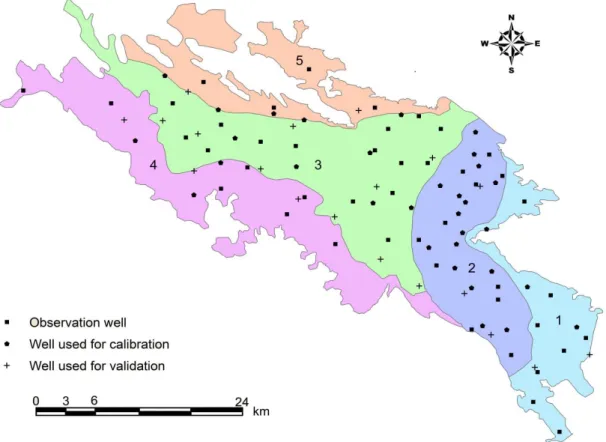
The studied region is Najafabad sub-basin shown in Figure 1. Najafabad is located between 50˚ 57˝ to 51˚ 44' 26˝ E and 32˚ 20'13˝ to 32˚49'21˝ N. The area of the site is approximately 1720.23 km2, and the aquifer area is about 1142.67 km2. Mean annual evapotranspiration is 1500 mm, and mean annual precipitation is only 158 mm, which occurs mostly in the winter months.
According to the past studies (Alijanian, 2008; Bahreini, 2006), the aquifer is being recharged through Karvan and Lenjanat aquifers and is a source for Isfahan- Borkhar and North Mahyar aquifers.
Najafabad aquifer (Figure 1) is located in Najafabad sub-basin. Important sources of recharge for the aquifer, in order of importance, are river, irrigation percolation- due to the water taken from groundwater wells and modern irrigation systems- and precipitation. The area is served by three modern irrigation networks: Right Nekoabad,
3 semi-positive definiteness of both matrices to be multiplied guaranteed semi-positive definiteness of the
left Nekoabad, and Khamiran. Withdrawals from the aquifer are for agricultural use in almost all cases (Isfahan Regional Water Authority 2007).
Figure 1. Najafabad aquifer divided into five zones for calibration and its wells
The iso-level lines of groundwater within the Najafabad aquifer domain in the first month of the modeling and unit hydrograph of the aquifer for whole modeling period taken from Isfahan regional water authority are shown in Figure 2.
Modeling details
The model is a Mesh-centered finite difference which is implemented in Matlab© R2009a. It has cell size of 500 ×500 m, monthly stress periods and time span from October 2000 to September 2007.
Because nearly all uses of water in the region is agricultural, all extractions from or recharge to the aquifer, except precipitation, are intensified to green surfaces. Each green surface relates to an irrigation network and was imported to GIS.
According to the available discharge information, monthly aquifer extractions are considered with three distinct values in each green surface. The recharge due to irrigation losses as a percentage of water incoming to the networks and 0.3 of withdrawal values of each surface was exerted equally in the cells of each of these three surfaces. The percentage of incoming water of the irrigation networks recharging the aquifer are selected based on the previous studies (Alijanian, 2008; Bahreini, 2006). Monthly rainfall amounts based on Najafabad station records are distributed equally in all cells of the aquifer. This assumption is acceptable because almost all the lands in the region are almost flat or with gentle slope.
Figure 2: Iso-level lines of groundwater within Najafabad aquifer domain (October
2000) and unit hydrograph of the aquifer (Oct. 2000-Sep. 2007)
Model boundary conditions include no flow boundaries in the north, south and the west and specified head boundaries in the border of Isfahan- Borkhar aquifer, in the northeast, Lenjanat aquifer in the southeast and Mahyar aquifer in the east. The aquifer was divided into five zones for modeling based on geological characteristics and previous modeling studies (Alijanian 2008; Bahreini 2006). Constant Hydrogeologic coefficients for each zone were considered (Figure 2).
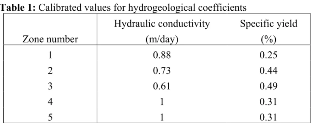
Hydrogeological coefficients of these five zones were derived through calibration with the index of sum of squared differences between monthly values of 32 observation wells data (of total number of 49 observation wells) since October 2000 to March 2005 (54 months). The results are summarized in Table 1 and are consistent with previous studies results (Alijanian, 2008; Bahreini, 2006).
Table 1: Calibrated values for hydrogeological coefficients Specific yield (%) Hydraulic conductivity (m/day) Zone number 0.25 0.88 1 0.44 0.73 2 0.49 0.61 3 0.31 1 4 0.31 1 5
The aquifer was modeled with these calibrated parameters from April 2005 to September 2007. Modeling results are compared with 17 observation well records and the model showed a good performance. It should be mentioned that because of the assumption that the calibrated model results as true data, the calibration is not effective in evaluation of filter performance.
Filtering details
Simulation results for all grid nodes within the aquifer for 84 months were recorded. The results were treated as actual data in assessment of the filter performance. Records of 45 randomly selected cells in the simulation were treated as observation data for use in filtering process. Observational error is assumed as a Gaussian stochastic process with zero mathematical expectancy (white noise) and variance of 0.01 m2 and added artificially to the observed values. This variance value was recommended by the local water authority experts and is based on the precision of measuring instruments for the observation wells. We made the effort to select 45 cells so that they contain all types of discharge and recharge regimes existing in the region. The position of all observation wells and points selected as the observation wells in the filtering procedure, are shown in Figure 2.
Hydraulic conductivity values of the aquifer for the five zones were adjusted by factors of 2, 5 and 10 respectively, in three different simulations. A set of observations from the simulation with the calibrated values of the coefficients are available for comparisons. The results of the simulation with inaccurate parameters assimilated within the ensemble Kalman filter with 100 ensemble members with and without localization
were evaluated. Localization with three length-scale parameters (5 ×500, 7 ×500 and 10 ×500 m) was implemented. The results of each run compared with the simulated results with the calibrated values as actual data for all cells of the model domain.
Filter performance evaluation
For evaluating performance of the filter that consists of a model with inaccurate parameters with and without localization, the best criteria can be defined as square root of mean squared differences between filter results and true model values. In other words, if Xˆ is the vector of filter results and X is the vector of true model results, then the t
statistical criteria RMSE can be defined as:
∑
= ⎟ ⎠ ⎞ ⎜ ⎝ ⎛ − = n i i t i x x n RMSE 1 2 ˆ 1where xˆi is the i th element of vector, Xˆ and X are the i th element of vector t X t and n is the size of both vectors which is equal to the dimension of the system.
Summary of Results
As expected, RMSE values for cases of inaccurate parameters model have lower variance when compared with accurate parameter model values and were generally lower. This point highlights the fact that the deterministic ensemble Kalman filter can make a significant contribution for adjusting the results of any inaccurate model. The
RMSE values for all 6 inaccurate models are shown in Figure 3.
Filter Performance without Localization
In the case of inaccurate hydraulic conductivity values (with factors of 2, 5 or 10 times of the accurate ones), the RMSE values for the filter without localization are small and reasonable. The RMSE values for these three non-localized filters have severe reduction in the first few steps and then they show smooth curves and a considerable drop is not observed. Figure 4 shows the results. For some of the ensemble sizes smaller than 100, trends of RMSE values don't form smooth and stable curves within the period. To show the reasonableness of the results and also to satisfy the paper length requirements only the results of the ensemble size of 100 are reported here.
Figure 3: RMSE values for inexact models with inexact hydraulic conductivity
Conclusions
DEnKF method makes significant contribution to correct the results of any inaccurate model. The use of DEnKF for groundwater flow modeling shows remarkable improvement in simulation results. Usually this improvement is shown mainly in the first few time steps. As it is shown in Figure 4, localization with all three length scales improved the filter performance in all cases. However, in the case of two or five times of the true hydraulic conductivity this improvement is maximized at length scale of 5000 m and in the other case 3500 m of length scale seems to be the best.
Localization of the filter causes a change in secondary rising trend of error and makes it a falling trend. f
e
P is not presented directly in the equations of most ensemble filters. When their square root or other forms exist, applying the localization is not directly possible. Therefore, localization often leads to computational difficulties. It is very unlikely that localization can be is easily performed due to the presence of f
e
P in the equations of DEnKF. On the other hand, as mentioned before, localization provides
better filter results in all cases. Therefore, localization (with this tapering function) is always recommended.
Figure 4: RMSE values for filter a) with 2×Kexact b) with 5×Kexact c) with 10×Kexact
If the length-scale for localization is larger than the optimum value, it cannot set spurious correlations to zero for relatively far distances (in error covariance matrix). In other words, false correlations remain in the range of the length-scale in this case. If the selected length-scale is smaller, the filter is not effective enough to adjust the model due to setting some real dependencies to zero artificially.
References
Alijanian, M. A. (2008). “Conjunctive use and management of surface water and groundwater with fuzzy logic”, Ms. Thesis, Isfahan University of Technology (IUT), Isfahan, Iran.
Anderson, J. L. (2001). “An ensemble adjustment Kalman filter for data assimilation.” J. Mon. Weather Rev., 129, 2884–2903.
Bahreini, Gh. R. (2006). “Surface and groundwater interaction modeling under uncertainty with reliability analysis.” Ms. Thesis, IUT, Isfahan, Iran.
Bishop, C. H., Etherton, B. J., and Majumdar, S. J. (2001). “Adaptive sampling with the ensemble transform Kalman filter Part I: Theoretical aspects.” J. Mon. Weather Rev., 129, 420–436.
Burgers, G., Van Leeuwen, P. J., and Evensen, G. (1998). “Analysis scheme in the ensemble Kalman filter.” J. Mon. Weather Rev., 126, 1719–1724.
Chen, Y., and Zhang, D. (2006). “Data assimilation for transient flow in geologic formations via Ensemble Kalman filter.” J. Adv. Water Resour., 29, 1107-1122. Drécourt, J. P., Madsen, H., and Rosbjerg, D. (2006a). “Bias aware Kalman filters: Comparison and improvements.” J. Adv. Water Resour., 29, 707-718.
Drécourt, J. P., Madsen, H., Rosbjerg, D., (2006b). “Calibration framework for a Kalman filter applied to a groundwater model” J. Adv. Water Resour., 29, 719-734.
Evensen, G. (1994). “Sequential data assimilation with a nonlinear quasi-geostrophic model using Monte Carlo methods to forecast error statistics.” J. Geophys. Res., 99(10), 143–162.
Evensen, G. (2003). “The ensemble Kalman filter: Theoretical formulation and practical implementation.” J. Ocean Dyn., 53, 343–367.
Gaspari, G., and Cohn, S. E. (1999). “Construction of correlation functions in two and three dimensions.” Q. J. Roy. Meteor. Soc., 125, 723–757.
Hunt, B. R., Kostelich, E. J., and Szunyogh, I. (2007). “Efficient data assimilation for spatiotemporal chaos: A local ensemble transform Kalman filter.” J. Physica Dyn., 230,112–126.
Isfahan Regional Water Authority, (2005). “Zayandehrood River Basin Report.” IRWA, Isfahan, (in Persian).
Krešić, N. (1997). Quantitative solutions in hydrogeology and groundwater modeling, Lewis Publishers, Boca Raton.
Ott, E., Hunt, B., Szunyogh, I.,Zimin, A. V., Kostelich, E., Corazza, M., Kalnay, E., Patil, D. J., and Yorke, J. A. (2004). “A local ensemble Kalman filter for atmospheric data assimilation.” J. Tellus, 56, 415–428.
Petrie, R. E. (2008). “Localization in the ensemble Kalman Filter.” Ms. Thesis, Department of Meteorology, University of Reading, UK.
Sakov, P., and Oke, P. R. (2008). “A deterministic formulation of the ensemble Kalman filter: An alternative to ensemble square root filters.” J. Tellus, 60, 361– 371.
Sun, A. Y., Morris, A., and Mohanty, S. (2009). “Comparison of deterministic ensemble Kalman filters for assimilating hydrogeological data.” Adv. in Water Resour., 32, 280-292.
Tippett, M. K., Anderson, J. L., Bishop, C. H., Hamill, T. M., and Whitaker, J. S. (2003). “Ensemble square-root filters.” J. Mon. Weather Rev., 131, 1485–1490. Van Geer, F. C. (1987). “Application of Kalman filtering in the analysis and design of groundwater monitoring networks.” PhD Thesis, Technical University of Delft, the Netherlands.
Whitaker, J. S., and Hamill, T. M. (2002). “Ensemble data assimilation without perturbed observations.” J. Mon. Weather Rev., 130, 1913–1924.