Progress in Paleoclimate Modeling*

HAL Id: hal-02930193

https://hal.archives-ouvertes.fr/hal-02930193

Submitted on 5 Apr 2021

HAL is a multi-disciplinary open access

archive for the deposit and dissemination of

sci-entific research documents, whether they are

pub-lished or not. The documents may come from

teaching and research institutions in France or

abroad, or from public or private research centers.

L’archive ouverte pluridisciplinaire HAL, est

destinée au dépôt et à la diffusion de documents

scientifiques de niveau recherche, publiés ou non,

émanant des établissements d’enseignement et de

recherche français ou étrangers, des laboratoires

publics ou privés.

Mark Cane, Pascale Braconnot, Amy Clement, Hezi Gildor, Sylvie Joussaume,

Masa Kageyama, Myriam Khodri, Didier Paillard, Simon Tett, Eduardo

Zorita

To cite this version:

Mark Cane, Pascale Braconnot, Amy Clement, Hezi Gildor, Sylvie Joussaume, et al.. Progress in

Paleoclimate Modeling*. Journal of Climate, American Meteorological Society, 2006, 19 (20),

pp.5031-5057. �10.1175/JCLI3899.1�. �hal-02930193�

Progress in Paleoclimate Modeling*

MARKA. CANE,⫹ PASCALEBRACONNOT,# AMY CLEMENT,@ HEZIGILDOR,& SYLVIEJOUSSAUME,# MASAKAGEYAMA,# MYRIAMKHODRI,⫹ DIDIERPAILLARD,# SIMONTETT,**ANDEDUARDOZORITA⫹⫹

⫹Lamont-Doherty Earth Observatory, Columbia University, Palisades, New York

# Institut Pierre Simon Laplace/Laboratoire des Sciences du Climat et de l’Environnement, UMR CEA-CNRS, Gif-sur-Yvette, France @ Rosenstiel School of Marine and Atmospheric Sciences, University of Miami, Miami, Florida

& Department of Environmental Sciences, Weizmann Institute of Science, Rehovot, Israel ** Hadley Centre, Met Office, Exeter, and University of Reading, Reading, United Kingdom

⫹⫹GKSS Forschungszentrum, Geesthacht, Germany

(Manuscript received 16 September 2004, in final form 14 August 2005) ABSTRACT

This paper briefly surveys areas of paleoclimate modeling notable for recent progress. New ideas, in-cluding hypotheses giving a pivotal role to sea ice, have revitalized the low-order models used to simulate the time evolution of glacial cycles through the Pleistocene, a prohibitive length of time for comprehensive general circulation models (GCMs). In a recent breakthrough, however, GCMs have succeeded in simu-lating the onset of glaciations. This occurs at times (most recently, 115 kyrB.P.) when high northern latitudes are cold enough to maintain a snow cover and tropical latitudes are warm, enhancing the moisture source. More generally, the improvement in models has allowed simulations of key periods such as the Last Glacial Maximum and the mid-Holocene that compare more favorably and in more detail with paleoproxy data. These models now simulate ENSO cycles, and some of them have been shown to reproduce the reduction of ENSO activity observed in the early to middle Holocene. Modeling studies have demonstrated that the reduction is a response to the altered orbital configuration at that time. An urgent challenge for paleocli-mate modeling is to explain and to simulate the abrupt changes observed during glacial epochs (i.e., Dansgaard–Oescher cycles, Heinrich events, and the Younger Dryas). Efforts have begun to simulate the last millennium. Over this time the forcing due to orbital variations is less important than the radiance changes due to volcanic eruptions and variations in solar output. Simulations of these natural variations test the models relied on for future climate change projections. They provide better estimates of the internal and naturally forced variability at centennial time scales, elucidating how unusual the recent global temperature trends are.

1. Introduction

Paleoclimate is a larger and grander topic than Cli-mate Variability and Predictability (CLIVAR), the subject of this entire special section. It encompasses a far greater range of time scales and a greater range of physical and biogeochemical processes. A decade ago, the mismatch between computing capability and the

length of integrations demanded by most paleoclimate problems severely limited what could be accomplished with general circulation class models. The great expan-sion of computing resources in the last decade still leaves a mismatch, but much more can now be done, and much more has been done. Moreover, the great improvement in climate models has made them far more useful tools in paleoclimate research. Key results reviewed in section 3, for example, depend on a coupled ocean–atmosphere model whose climate bears more than a passing resemblance to reality. Other problems require models for land surface processes, ocean chemistry and biology, and the cryosphere, com-ponents that were inadequate or nonexistent not long ago. (They are still inadequate for many problems, but progress has been impressive.) In seeking the causes of abrupt climate change, or the character of

glacial–inter-* Lamont-Doherty Earth Observatory Contribution Number 6811.

Corresponding author address: Mark A. Cane,

Lamont-Doherty Earth Observatory, Columbia University, 61 Route 9W, Palisades, NY 10964-8000.

E-mail: mcane@ldeo.columbia.edu

© 2006 American Meteorological Society

glacial cycles, none of these processes can be dismissed out of hand. This need to consider the climate system in the broadest terms is not only a grand intellectual chal-lenge, but has become distressingly relevant as we force the climate system beyond the limits of what is in the instrumental record.

Paleoclimate, in common with other earth sciences, is data driven. The decade’s advances in modeling are unimaginable without the enormous increase in the quantity and precision of paleoclimate proxy data. Two of the topics we discuss below, paleo-ENSO and abrupt change, did not exist until there were methods to create high-resolution records. For other topics, the observa-tional picture has become far less fuzzy, allowing many more tests of model against data. Though serious dating issues remain, the widespread use of time scales based on ice cores has allowed disparate data to be brought together with far greater confidence.

A decade ago it might have been possible to do a reasonably comprehensive review of paleoclimate mod-eling as a journal article. Now it would require book-length treatment. Rather than attempt the impossible, here we have chosen a few key topics judged to have some particular lessons and points of contact with CLIVAR science. This has meant leaving out huge tracts of fascinating and important science. We include nothing from earlier than about 800 000 yr (800 kyr) ago, omitting the important questions of why there was a transition from a dominant period of 41 kyr to one of 100 kyr at that time and why glaciation set on 2.73 Myr ago. We say little to nothing about interesting recent work on the role of lithospheric rebound, greenhouses gases, equable climate, the Eocene, the impact of tec-tonic changes, and a host of other topics. The topics we do treat are not covered comprehensively in most cases; instead a few examples are pursued to some depth. Individual sections are independent of each other, but the whole paper is greater than the sum of the sections. In section 2 we discuss recent modeling work on the causes of the glacial–interglacial cycles prominent in the last 800 kyr. Since it is not feasible to integrate GCMs for hundreds of thousands of years, this topic remains largely the domain of low-order models. The importance of threshold behavior is emphasized, as is the idea that orbital changes are the pacemaker of the climate system rather than the driver. In this view, posi-tive feedbacks internal to the climate system are re-sponsible for the 100-kyr cycle, with the orbital forcing setting its phase. We discuss one particular low-order model at some length. This model gives a lead role to sea ice, an idea with clear implications for future cli-mate.

Section 3 reports important progress on a key

ele-ment of glacial cycles, the onset of glaciation. This work features GCMs and demonstrates the critical impor-tance of water vapor transports. It also shows that the data cannot be explained without taking account of coupled ocean–atmosphere dynamical processes. Sec-tion 4 reviews progress in GCM simulaSec-tions of two sig-nature periods, the Last Glacial Maximum (LGM) and the middle Holocene. Results from the Paleoclimate Model Intercomparison Project (PMIP), which consti-tute a multimodel report on the state of the art, have clarified the role of the ocean and vegetation feedbacks in the climate system.

Section 5 addresses the least understood of our topics, abrupt climate change. The discussion here is largely conceptual, reflecting our lack of understanding of the causes of the abrupt climate changes in the pa-leoproxy record, and our very limited progress in mod-eling these changes. While the paradigmatic abrupt changes, Dansgaard–Oeschger cycles and Heinrich events, are millennial, the transitions between warm and cold states occur within decades. We are now over-lapping with CLIVAR time scales. Section 6 shows that we have gained an understanding of the variations in the character of the El Niño–Southern Oscillation (ENSO) cycle seen in paleoproxy data. The richest ob-servational picture is in the Holocene, and model simu-lations capture the major features. The Bjerknes feed-back (explained below), which is at the core of our understanding of the model ENSO cycle, turns out to be the key to understanding how small changes in or-bital configuration lead to substantial changes in ENSO. Section 7, which discusses modeling of the past millennium, intersects with CLIVAR time scales and CLIVAR issues. A key question is how much of the climate variability in the past 1000 yr is attributable to irradiance changes due to volcanic eruptions and solar variability. There are obvious implications for the cli-mate of the twentieth century, and the century to come. Section 8 offers concluding remarks.

2. Low-order models of glacial cycles

a. Phenomenology

Various paleoclimate proxies (Petit et al. 1999; Im-brie et al. 1984) indicate that during the past 800 000 yr (the late Pleistocene), the glacial–interglacial cycles were characterized by a pronounced 100 000 yr (100 kyr) oscillation, with additional weaker spectral peaks at 41 and 23 kyr and an asymmetric saw-tooth structure marked by the slow buildup of ice sheets and the rela-tively abrupt melting. In the cool phase global average temperature is about 5°C colder than today and sea level is about 120 m lower.

Variation in incoming solar insolation resulting from secular changes in the eccentricity of the earth’s orbit around the sun, in the tilt of the earth’s axis relative to the plan of orbit (obliquity), and in the precession of the equinoxes seems a natural candidate for a glacial theory given its time scale and potential climatic effects. As reviewed by Paillard (2001), such theories were pro-posed as early as the nineteenth century. These theories are now referred to as the Milankovitch theory or the astronomical theory. The mathematician Milankovitch suggested that the solar radiation during the boreal summer season is the critical climatic factor, as cold summers allow the survival of new snow cover from the previous winter season. He also accurately calculated the time variations of the different orbital parameters (Milankovitch 1941). However, the dominant peaks in the power spectrum of the insolation are those of the precession and obliquity, which suggest dominant fre-quencies of 19-, 23-, and 41-kyr periods, which is not in agreement with the dominant 100-kyr climatic signal.

A satisfying model, or mechanism, for the glacial– interglacial cycles should explain the following ob-served characteristics.

1) The roughly 100 kyr between glacial maximum dur-ing the past 800 kyr.

2) The asymmetric sawtooth structure of long glacia-tions (⬃90 kyr) and short deglaciaglacia-tions (⬃5–10 kyr).

3) The relatively good correlation with Milankovitch solar variations despite the small changes in earth insolation on a 100-kyr time scale.

4) The nearly synchronous changes in both hemi-spheres.

5) The glacial–interglacial atmospheric CO2variations.

During glaciation, atmospheric concentration of CO2 gradually declines and reaches a minimum of

about 200 ppm during glacial maximum, and it then rises relatively rapidly to a concentration of about 280 ppm at the end of the glacial termination. If one relies on the Milankovitch theory to explain the ice ages, additional issues should be addressed (Paillard 2001; Parrenin and Paillard 2003; Karner and Muller 2000; Imbrie et al. 1993).

6) The absence of cycles at 400 kyr, the major period-icity of eccentrperiod-icity.

7) The stage-11 problem (transition V). Approxi-mately 400 kyr ago, the earth’s orbit was almost circular. Hence seasonal changes in insolation were very small. Milankovitch theory predicts a small gla-cial–interglacial transition but, it was probably the most intense (Fig. 1).

8) The stage-7 problem (transition III). Approximately 230 kyr ago eccentricity was large, but the transition to interglacial was very mild (Fig. 1).

FIG. 1. (from top to bottom) Obliquity, June solstice insolation at 65°N, modeled ice volume, and proxies for ice volume from Bassinot et al. (1994) and SPECMAP (Imbrie et al. 1984). Bold roman numerals are terminations, and light decimal numbers indicate marine isotope stages (from Parrenin and Paillard 2003).

9) Why does termination II (approximately 135 kyr ago) lead the rise in insolation?

Models proposed for the 100-kyr cycles generally di-vide into those models having self-sustained oscillations and models driven by external forcing, or into nonlin-ear and linnonlin-ear models (see the reviews by Imbrie et al. 1993; Elkibbi and Rial 2001). Suggested mechanisms include a nonlinear transfer of energy from the Milan-kovitch forcing at higher frequencies to the 100 kyr (Le Treut and Ghil 1983), isostatic adjustments of the lith-osphere under the weight of the glacier (Oerlemans 1982), slow CO2feedback (Saltzman and Maasch 1988),

thermohaline circulation feedbacks (Ghil et al. 1987; Broecker and Denton 1990) and interplanetary dust (Muller and McDonald 1995).

b. Multiple equilibria and thresholds

Paillard (1998) suggested a very “pure” conceptual model, one with virtually no commitment to specific physical processes. Its high degree of abstraction makes it especially illuminating. Milankovitch forcing is im-posed on a glacial–interglacial cycling mechanism con-sisting of jumps between three modes of the climate system: interglacial (i), mild glacial (g), and full glacial (G). Rules are specified for the transition between these modes:

• i→ g (glaciation begins) occurs when the insolation

decreases below a threshold i0.

• g→ G (glaciation approaching its maximum) occurs

when the ice volume increases above some threshold value Vmax.

• G → i (deglaciation) occurs when the insolation

in-creases above some threshold i1⬎ i0.

Parrenin and Paillard (2003) modified this model so that deglaciation occurs when a combination of insola-tion and ice volume is above a threshold. This modifi-cation improves the agreement between the model re-sults and the climate records. The fit is very impressive, satisfying many of the above-mentioned observed char-acteristics of the glacial cycles (Fig. 1). Still, this model does not explain the actual physical mechanism or, say, what components of the climate system are responsible for the thresholds/multiple modes, etc., although a few hypotheses exist (Paillard 2001, 1998). This simple model implies that thresholds, a feature common to most of the low-order glacial–interglacial models, are essential elements of any glacial cycling mechanism. In the next section we give an example of a recent model of this kind that is fleshed out with explicit (though schematic) physical mechanisms.

c. A sea ice switch model

The importance of sea ice in the climate system has long been recognized (e.g., Saltzman and Moritz 1980). Sea ice presence and evolution affect the surface albedo and the salinity budget in the ocean. By partially insu-lating the ocean from the atmosphere it also changes air–sea heat flux, CO2flux, and evaporation.

Neverthe-less, most theories and simple models have no role for sea ice. Because of the strong seasonal cycle of sea ice, it was taken as a fast-response climatic variable that equilibrates with global temperature changes (Källén et al. 1979; Saltzman and Sutera 1984). Such a treatment does not allow for a transition between the different qualitative regimes of sea ice cover.

Gildor and Tziperman, (2000, 2001a,b) proposed a mechanism in which sea ice acts as a “switch” of the climate system, switching it from glaciation to deglacia-tion. It is based on the somewhat debated (Gildor 2003a,b; Alley 2003) “temperature–precipitation feed-back” (Le Treut and Ghil 1983), in which the rate of snow accumulation over land ice sheets increases with temperature, outweighing the corresponding increase in ablation and melting. Via its strong cooling albedo effect, its insulation effect on local evaporation, and its role in diverting the storm track, the sea ice controls the atmosphere moisture fluxes and precipitation that en-able land ice sheet growth. The rapid growth and melt-ing of the sea ice allow the sea ice to switch the climate system rapidly from a growing ice sheet phase to a re-treating ice sheet phase, shaping the oscillation’s saw-tooth structure.

Gildor and Tziperman use a global meridional box model (fully described in Gildor et al. 2002) composed of ocean, atmosphere, sea ice and land ice submodels, including active ocean biogeochemistry and variable at-mospheric CO2. Consider the full oscillation between

years 170 000 and 70 000 in Fig. 2. Starting from an interglacial, the ocean is ice free (Fig. 2b) and the at-mospheric temperature (Fig. 2d) and oceanic tempera-tures in the northern box are rather mild. The amount of precipitation enabling ice sheet growth in the north-ern polar box exceeds the melting and calving terms (Fig. 2c, year 170 000), and therefore the ice sheet gradually grows. The northern box atmospheric tem-perature while relatively mild, is below freezing, en-abling the glacier to grow. The spreading of the land ice sheet increases the albedo, and consequently the tem-perature of the atmosphere and of the ocean in the corresponding polar box decreases slowly with the growing glaciers (Fig. 2d). Eventually, around year 90 000, the sea surface temperature (SST) reaches the critical freezing temperature, and sea ice (Fig. 2b) starts

to form very rapidly. The creation of sea ice further increases the albedo, reduces the atmospheric tempera-ture, and enhances the creation of more sea ice. The characteristic time scale of sea ice growth is very short, and in less than 50 yr nearly the entire polar box ocean surface is covered by sea ice. The sea ice switch is now turned to “on.”

At this stage, the average global temperature is at its lowest point, sea ice and land ice sheet extents are maximal, and the system is at a glacial maximum. Be-cause of the low polar box atmospheric temperature (Fig. 2d, year 85 000), poleward moisture flux declines to about half its maximum value. In addition, the sea ice cover limits the moisture extraction by evaporation

from the polar ocean box and further reduces the cor-responding snow accumulation over the land ice. Being less sensitive to temperature than precipitation, abla-tion and glacier runoff dominate, so the glaciers start retreating. The land albedo decreases and the atmo-spheric temperature rises slowly. This is the beginning of the termination stage of the glacial period. The upper ocean in the polar box is at the freezing temperature as long as sea ice is present. However, once the deep ocean warms enough to allow the upper ocean to warm as well, the sea ice melts within⬃40 yr. [A similar rapid retreat of sea ice may have occurred at the end of the Younger Dryas (Dansgaard et al. 1989).] The sea ice switch is now turned to “off,” the temperature of both

FIG. 2. Low-order sea ice switch model result time series for 200 kyr with no orbital variations. (a) Northern land ice extent as a fraction of the polar land box area; (b) northern sea ice extent as a fraction of polar ocean box area; (c) source term (solid line) and sink term (dashed line), for northern land glacier (Sv, 1 Sv⬅ 106 _m3_s-1_{); (d) northern atmospheric}

temperature (°C); (e) atmospheric CO2(ppm); and (f) southern sea ice extent as a fraction of

polar ocean box area. Time is in “before present” model years, although no correspondence to actual time before present is meant; such correspondence is relevant only when Milanko-vitch forcing is included, and the results shown here were obtained when orbital parameters were held at their present values. (After Gildor et al. 2002.)

the atmosphere and the ocean are at their maximum values, and the system is at an interglacial state, having completed a full glacial cycle. The cycle in glacier vol-ume is equivalent to about 100 m of sea level change.

While not the direct forcing of the 100-kyr oscilla-tions in this mechanism, Milankovitch forcing affects the characteristics of the 100-kyr cycle through nonlin-ear phase locking (Saltzman et al. 1984; Imbrie et al. 1993). When the model is forced with ablation as a function of summer insolation at 65°N, runs with dif-ferent initial conditions for the northern polar ice sheet extent all converge into a single time series after about 130 kyr (Gildor and Tziperman 2000). Milankovitch forcing is the pacemaker for the glacial cycles.

While the model used to demonstrate the sea ice switch mechanism is fairly idealized, its representation of the various climate components is sufficiently ex-plicit for it to make predictions that can be tested with fuller GCMs and possibly with analysis of proxy records of sea ice as these become available. The main predic-tion of this model is the hysteresis of land ice and sea ice, namely different states of sea ice cover for advanc-ing and retreatadvanc-ing sea ice (Sayag et al. 2004). This model also predicts that the onset of the land deglacia-tion should correspond to a larger sea ice cover, and hence a colder period, and that extensive sea ice cover exists well into deglaciation. Hence there is no simple relationship between ice volume and temperature (cf. Paillard 2001).

d. Stochastic models

Generally, natural time series may be described by a set of dynamical equations with both deterministic and stochastic elements. The extent to which climatic rec-ord can be explained by the Milankovitch theory is still controversial. For example, Paillard (2001) suggests that the climate system is mainly deterministic on the glacial–interglacial time scale, while Wunsch (2003) suggests that Milankovitch forcing can explain only a small fraction of the variability.

Wunsch (2003) demonstrates that it is possible to replicate a realistic-looking time series for ice volume by a simple stochastic model that includes a threshold. In the Wunsch model, ice volume V(t) builds up ran-domly to a specified maximal threshold at which point it breaks up rapidly. Then, growth begins again. The ice volume thus fluctuates between the maximal threshold and zero, and the ice volume growth is similar to a simple linear random walk. Note that this model relies on thresholds and is nonlinear. Ashkenazy et al. (2005) suggest models with both deterministic and stochastic elements, which account for some of the stochastic non-linear features of ice core (Ashkenazy et al. 2003).

Benzi et al. (1982) suggested stochastic resonance as a mechanism for glacial cycles. Stochastic resonance may occur in a system with two stable equilibria (e.g., a cold glacial state and a warm interglacial state) sepa-rated by a threshold. The system is driven by both ran-dom noise and by slow and small-amplitude periodic oscillations due to Milankovitch forcing. The periodic force by itself cannot drive the system above the thresh-old, but the right combination of noise amplitude and periodic forcing can cause a transition. Because this mechanism is expected to produce symmetric oscilla-tions, it is probably not the main reason behind the 100-kyr cycle (Tziperman 2001; Pelletier 2003).

Pelletier (2003) suggested a simple model based on coherence resonance to explain the glacial–interglacial cycles. As in stochastic resonance, there is a system with two stable equilibria separated by a threshold, but un-like stochastic resonance, coherence resonance relies on the nonlinear dynamics of the system rather than an external periodic forcing. It requires a delayed feed-back in the system, that is, a forcing that depends on the state of the system at a previous time (Tsimring and Pikovsky 2001; Pelletier 2003). In the model of Pelle-tier, isostatic adjustment of the lithosphere provides the delayed feedback. In coherence resonance, occasionally the noise drives the system enough in the same direc-tion to cross the threshold. The chance for this to occur depends on the time scale of the delayed feedback and the level of noise. This model reproduces the saw-tooth structure of the climate record and the 100-kyr time scale. Timmermann et al. (2003) present an alternate coherence resonance scenario.

e. Discussion: Low-order models

Many low-order models fit the global ice volume proxy curves quite impressively, perhaps not a surprise considering the number of tunable coefficients in them (Tziperman 2001; Roe and Allen 1999) and uncertain-ties in the data. It seems likely that any model that has a free nonlinear oscillation at about the 100-kyr period and that is forced by Milankovitch forcing will be phase locked to the forcing and will result in a good fit to the global ice volume proxy curves. Obviously models driven by Milankovitch forcing will show coherence with the data. Phasing between the hemispheres and between climate parameters (as temperature and ice volume) is ambiguous, partly due to millennial-scale variability superimposed on the glacial cycle signal (Alley et al. 2002), partly because each proxy for ice volume (like ␦18_{O from planktonic and benthic}

fora-minifera) is also affected by other factors (such as tem-perature, salinity, and pH; e.g., Mix et al. 2001), and partly because the data may be biased by seasonality of

the specific proxy (Gildor and Ghil 2002). In addition, phasing between climate variables such as ice volume and temperature may change in time, making it difficult to distinguish between cause and effect (Karner and Muller 2000). There is a need to develop ways to dis-tinguish between competing explanations that all fit a few data time series; the models must make new and independent testable predictions. Despite major ad-vances in the last few decades, the increasing number of models for the ice ages in recent years is evidence that we still lack a satisfying explanation of the dynamics of the large-amplitude glacial climate cycles.

3. Glacial inception

a. Phenomenology

The last glacial inception has been the focus of many modeling studies primarily because it is the one best documented by proxy data and thus provides precious information concerning the environmental changes that lead to glaciation. The preceding interglacial, the Ee-mian, is the last interval in which the global climate was close to that of the present day. The correlative marine isotope substage (MIS) 5e, as recorded by the marine oxygen isotopic composition, shows that this period of minimum ice volume lasted some 12 000 yr starting at about 128 000 yr before present (128 kyrB.P.). At the late boundary of the Eemian, 116 kyr B.P. (the MIS 5e/5d transition in ocean records), the climate started to cool down, marking the beginning of the most recent glacial stage (Shackleton et al. 2002; Chapman and Shackleton 1999). Coral reef and marine oxygen isoto-pic records from different regions in the world indicate a global sea level drop of between 2 and 7 m over 1 kyr during the early stage of the interglacial–glacial transi-tion (Lambeck and Chappell 2001; Shackleton 1987), but little is known of the location of the initial water storage in ice sheets that ultimately grew to cover North America (the Laurentide ice sheet) and northern Eu-rope (the Fennoscandian ice sheet).

b. Past theories and models

The last transition to a glacial climate was at a time when northern high-latitude summer insolation was at a minimum, in accord with the Milankovitch theory (sec-tion 2a). The earliest attempts to test this theory in-volved simple conceptual models that tried to repro-duce ice age cycles driven only by summer insolation changes at 65°N, the latitude near a glaciation threshold according to Milankovitch (e.g., Imbrie and Imbrie 1980). Experiments with two-dimensional energy bal-ance models (EBMs) coupled to an ice sheet model

and/or a mixed layer ocean have had some success in reproducing the major characteristics of glacial– interglacial cycles, but only by applying reconstructed atmospheric CO2variations in addition to the cycles of

insolation forcing (Tarasov and Peltier 1997, 1999). Ini-tial experiments with atmospheric general circulation models (AGCMs) consisted of changing the orbital pa-rameters to their 116 kyr B.P. values while assigning

present-day values to vegetation, ocean temperatures, and sea ice. The climatic adjustment was analyzed in terms of cooling and snowfall distributions. The results were disappointing: changing only solar insolation failed to produce perennial snow. How snowmelt is pa-rameterized and the impact of the model resolution on the effect of altitude on snow nucleation, as well as the bias in the simulated present-day climate, are all rea-sons that might explain the difficulties encountered by GCMs in reproducing glacial inception (Vettoretti and Peltier 2003). However, with the substantial increase in the number of proxy and modeling studies of the last glacial inception during the last decade, it has been concluded that most of these experiments had two ma-jor weaknesses. First, the atmosphere did not cool the climate enough to prevent snow from melting. Second, and most important, the cooling made the atmosphere drier, preventing any increase in snowfall.

In the 1990s, new evidence of important vegetation changes over northern Canada and Europe at the end of the last interglacial (e.g., Pons et al. 1992) led to the idea that the recurring difficulties with most of these GCM studies were not only due to their biases, but might be linked to missing climatic feedbacks. Galli-more and Kutzbach (1996) performed sensitivity ex-periments in which boreal forests were replaced by tun-dra, while DeNoblet et al. (1996) used an AGCM asyn-chronously coupled to a vegetation model. With such changes prescribed, the increased land surface albedo helps to maintain snow cover over more than a seasonal cycle. Other experiments explored alternative feed-backs that may help to maintain perennial snow cover. The earliest simulations using an AGCM assumed that the sea surface temperatures were very similar to present day. To account for insolation changes on SST, Dong and Valdes (1995) coupled an AGCM to a mixed layer ocean and found that the ocean surface cools and sea ice cover expands. More importantly, the model delivered perennial snow cover over regions known to be the starting point of the ice sheets. This experiment was the first to reveal the role of the ocean in helping glacial inception. However, in light of recent data, the simulated summer cooling over high-latitude oceans of up to 8°C now appears unrealistic. Recent SST recon-structions show that the increased equator-to-pole

in-solation gradient around 115 kyrB.P. creates a cooling

of up to 3° to 4°C, at 72°N in the Norwegian Sea, while in the Atlantic Ocean low to mid latitudes remained warm even after the ice sheet started to build up (Cortijo et al. 1999; Chapman and Shackleton 1999; McManus et al. 2002; Shackleton et al. 2002).

c. Coupled ocean–atmosphere results

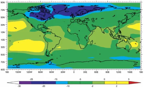
Model SSTs over the key North Atlantic region in the coupled atmosphere–ocean GCM (AOGCM) simu-lation of Khodri et al. (2001) are shown in Fig. 3. The geographical pattern of the data is generally repro-duced: the high latitudes of the North Atlantic cool while the tropical and subtropical latitudes remain warmer, more similar to the present day. After several years, the 115 kyr B.P. simulation produces perennial snow cover and then snow accumulation over the Ca-nadian Archipelago (also see Fig. 4 of Khodri et al. 2001).

In this study the ocean translates the seasonal anomaly of insolation into an annual mean amplifica-tion of the equator-to-pole SST gradient. As a conse-quence, the low-latitude water vapor source increases and provides an increased moisture availability for the high-latitude atmosphere. The hydrological cycle change has major impacts on high-latitude climate. The annual mean increase of runoff into the Arctic Ocean induces an extension and deepening of the halocline, which, associated with the cooler surface water, in-creases Arctic sea ice volume and extent. This change

in sea ice contributes to cooling of the land surrounding the Arctic Ocean, such as the Canadian Archipelago, by increasing local albedo. The increased freshwater input into the Arctic Ocean also induces a reduction of the sea surface salinity (SSS). Subsequently, the de-creased meridional density gradient in the northern seas leads to a shift of the location of deep-water for-mation toward lower latitudes, which, in turn, inhibits the convergent transport of heat by the ocean to those latitudes now covered by sea ice. Finally, the amplified high-latitude cooling by these feedbacks translates the increased atmospheric water vapor transport into in-creased snowfall over regions where ice sheets can grow. Including the ocean feedback provides more moisture to northern high latitudes. This is the essential effect that allows snow to accumulate, triggering the “Milankovitch effect.”

Earth Models of Intermediate Complexity (EMIC) include most of the components of the climate system, such as the ocean, biosphere/carbon cycle, sea ice, and ice sheets, but their representations are simplified so that several multimillennial transient simulations and sensitivity experiments can be performed without com-puting time restrictions. This is particularly important for the last interglacial–glacial transition since data show important transient changes. An “intra-Eemian” cooling around 122–120 kyrB.P. is seen in both marine

and continental data in several locations in Europe. A rapid shift to a colder climate and reduced sea surface salinity is recorded in high-latitude oceans during the

FIG. 3. Differences in simulated summer SSTs (°C) and land snow depth (cm) at the last glacial inception climate (115 kyrB.P.) from those simulated for the present-day climate (Control). Results are from a coupled ocean–atmosphere general circulation model (OAGCM) forced solely by orbital insolation changes. Values are between⫾ 3°C with 0.25°C contour intervals for SSTs, and between ⫾ 13 cm with 2-cm contour intervals for snow depth. The dotted (solid) isolines indicate a decrease (increase) in SSTs.

second part of the last interglacial near 120 kyr B.P.

(Cortijo et al. 1999; Maslin et al. 2001; Oppo et al. 2001; Sànchez-Goñi et al. 1999; Tzedakis et al. 2002), an event followed by another cooling step marking the end of the last interglacial, around 115 kyr B.P. (Chapman

and Shackleton 1999; Shackleton et al. 2002).

Using an EMIC, Crucifix and Loutre (2002) showed that the gradual reduction of summer insolation from 126 to 115 kyrB.P. induces a gradual expansion of the

Arctic sea ice, hastening the southward shift of the northern tree line by 1000 yr and allowing the accumu-lation of perennial snow cover over northern lands as early as 122 kyr B.P. Wang and Mysak (2002) also

re-produce glacial inception by coupling an EMIC to an ice sheet model. However, as in Crucifix and Loutre (2002), the reduced freshwater input to high-latitude oceans causes a gradual increase of SSS in the northern seas, whereas Cortijo et al. (1999) reported a freshening of the northern oceans from 122–120 kyrB.P. until 115 kyr B.P. Using a coupled ocean–atmosphere EMIC forced by insolation changes only, Khodri et al. (2003) also found that the SSS in the Northern Seas increased and that the model did not simulate perennial snow cover. However, when the northward atmospheric moisture transport was artificially amplified to mimic the AOGCM results, the EMIC was able to simulate the northern SSS decrease and perennial snow over northern Canada (Khodri et al. 2003).

Thus, a major finding of recent model studies of in-terglacial–glacial transition is the central role played by hydrological cycle changes. The increased northward moisture transport amplifies the high-latitude cooling initiated by the insolation change through an intricate network of feedbacks involving sea ice and the ocean, but it also moistens the atmosphere so snow delivery can increase.

4. Results from the Paleoclimate Modeling Intercomparison Project

a. Overview

The international Paleoclimate Modeling Intercom-parison Project (PMIP 2000), was created to assess the ability of models to simulate climates very different from the present day. PMIP has stimulated data syn-theses for two key periods in the past, the LGM (21 kyr

B.P.) and the mid-Holocene (6 kyrB.P.; e.g., Harrison 2000). PMIP1, the first phase of PMIP, considered only AGCMs. The last years have seen an increasing num-ber of coupled ocean–atmosphere and atmosphere– vegetation model paleoclimate studies, first for the mid-Holocene (see Braconnot et al. 2004), and more recently for the LGM (Hewitt et al. 2001; Kim et al.

2003; Kitoh et al. 2001; Shin et al. 2003a). Only a few simulations have incorporated both the ocean and veg-etation feedback (Braconnot et al. 1999).

b. The Last Glacial Maximum and the mid-Holocene

At the LGM there were 3- to 4-km-high ice sheets spread over North America and Scandinavia and the concentration of carbon dioxide was reduced to about 200 ppm. The mean global cooling was about 5°C. In PMIP1 the AGCMs were either forced by the CLIMAP (1981) reconstruction of SST or coupled to a simplified slab ocean model. In the coupled model experiments of PMIP2 only external conditions such as the CO2 level

and the ice sheet location and topography need to be prescribed (see http://www-lsce.cea.fr/pmip for more information).

Results of PMIP simulations exhibit a global cooling of about 4°C when SSTs are prescribed and from 2° to 6°C when SSTs are computed. The cooling is larger over land and ice-covered regions, because of the smaller thermal inertia of land and the large ice and snow albedo feedback (Fig. 4). The change in the lati-tudinal temperature gradient in the Atlantic Ocean to-gether with the orographic effect of the ice sheet favors an eastward shift of the core of the storm-track activity (Kageyama et al. 1999). Most coupled ocean–atmo-sphere simulations provide a similar range for the glob-al cooling (Hewitt et glob-al. 2001; Kim et glob-al. 2003; Kitoh et al. 2001; Shin et al. 2003a), though the simulated pat-tern of SST change varies greatly from one model to the other. For example, the Third Hadley Centre Coupled Ocean–Atmosphere GCM (HadCM3; Hewitt et al. 2001) simulation exhibits a warming in the North At-lantic not found in the National Center for Atmo-spheric Research (NCAR) Climate System Model (CSM; Shin et al. 2003a) coupled simulation (Fig. 5), apparently due to strong katabatic flow off the ice sheet, and a shift in the boundary of the subpolar gyre and the location of deep-water formation (Fig. 6). Gen-erally, the coupled simulations are an improvement over the AGCM results of PMIP1, reproducing obser-vations over land more accurately, and capturing the changes in the temperature gradient over the ocean (Kageyama et al. 2006). However, none of the available simulations sustains the cold conditions over Europe suggested from data or give a realistic representation of Atlantic SST and sea ice cover. A simulation with a high-resolution model yielded only a slight improve-ment (Jost et al. 2005).

In the tropical regions the LGM has a damped sea-sonal cycle. Since evaporation is reduced over the cold

ocean, the LGM climate is more arid. Models with specified SSTs tend to underestimate the tropical land cooling, but some of the models that compute SST are consistent with data reconstructions (Pinot et al. 1999). The difference in perihelion at mid-Holocene in-creased the incoming solar radiation at the top of the atmosphere about 5% in boreal summer compared to the present day. In response to the insolation forcing, the land–sea contrast responsible for the monsoon is enhanced in the Northern Hemisphere (NH). The in-tertropical convergence zone shifts to a more south-ward position over the ocean during winter and

pen-etrates farther inland during summer. All PMIP simu-lations show that the summer monsoon flow brought more precipitation in now arid regions such as the Sahel region in Africa or the northern part of India (Fig. 7). Moisture advection plays a more important role in West Africa than local recycling, though local recycling does account for at least 30% of the precipitation in this region. None of the PMIP1 simulations change humid-ity in the Sahel region enough to allow the northward encroachment of steppe vegetation into the desert that is seen in the data (Harrison et al. 1998; Joussaume et al. 1999). The timing and the length of the monsoon

FIG. 5. Change in annual mean surface temperature, LGM – Modern, for two coupled simulations: (top) HadCM3 (Hewitt et al. 2001) and (bottom) NCAR CSM (Shin et al. 2003a).

FIG. 4. Simulated change in annual mean surface temperature (°C) at the LGM. Average of 9 PMIP1 simulations with SST prescribed according to the CLIMAP (1981) reconstruction. Isolines are plotted at every 5°C, except that⫾2°C isolines are added to highlight temperature changes over the ocean. Data are from the PMIP database (http://www-lsce.cea.fr/pmip).

season is more consistent among the coupled simula-tions and the results are in better agreement with data (Braconnot et al. 2004).

c. Ocean and vegetation feedbacks

Simulated changes in SST and sea ice cover for the LGM are associated with changes in deep-water forma-tion in the North Atlantic. Table 1 summarizes some recent results related to the thermohaline circulation. Most of these coupled simulations shift the deep-water formation in the North Atlantic southward and weaken the overturning circulation, as illustrated in Fig. 6. Most of the simulations also reinforce the formation of Ant-arctic Bottom Water. Shin et al. (2003b) show that the dominant mechanism is an increase of surface density due to brine rejection when sea ice forms. Results from intermediate-complexity models and stability studies suggest that during cold states the thermohaline

circu-lation is close to a stability threshold (cf. section 5), and the different AOGCM results all appear to be plausible ocean states.

Coupled simulations of the mid-Holocene show little change in the overturning circulation. Analysis suggests that the buildup of a interhemispheric SST gradient across 5°N in the Atlantic feeds back on the strength-ening of the African monsoon (Zhao et al. 2005). Also, the late warming of the northwest Indian Ocean in au-tumn delays the monsoon retreat in this region. This feature is maintained through a feedback loop between a reduction of the mixed layer depth and the input of low salinity water at the surface that both contribute to reduce the local inertia of the surface ocean (Zhao et al. 2005). Precession sensitivity experiments suggest that these features are the signature of late summer–fall in-solation forcing during the mid-Holocene (Braconnot and Marti 2003).

FIG. 6. Change in annual mean surface temperature, LGM–Modern, for two coupled simulations: (top) HadCM3 (Hewitt et al. 2001) and (bottom) NCAR CSM (Shin et al. 2003).

Though changes in vegetation induce large feed-backs, they have less impact on the simulated climate than changes in the ocean circulation or in greenhouse gases. Shin et al. (2003a) estimated that changes in greenhouse gases account for half of the tropical cool-ing. Inclusion of the physiological effect of the CO2

concentration on vegetation is nonnegligible (Levis et al. 1999), impacting changes in the global forest (Har-rison and Prentice 2003). Dust loading and deposition

was larger during the LGM (e.g., Kohfeld and Harrison 2001), which has been attributed to changes in soil hy-drology and vegetation cover (Mahowald et al. 1999).

The African monsoon in the mid-Holocene illus-trates the synergy among the vegetation feedback, the ocean feedback, and the seasonal cycle of insolation (Braconnot et al. 1999). In response to the intensifica-tion of monsoon precipitaintensifica-tion (Fig. 7) the desert steppe transition is shifted to the north. The ocean feedback

TABLE1. Changes in LGM thermohaline circulation as inferred from various sources, including results from both EMICs and fully coupled OAGCMs.

Authors Model ⌬THC strength (Sv)

Convection sites

NADW depth Ganopolski et al. (1998;

Ganopolski and Rahmstorf 2001)

EMIC CLIMBER 2 Weakening (⫺4) 60°N→ 50°N Shallowing

Wang et al. (2002) EMIC atm EBM⫹ 2D ocean Strengthening

(0–6 depending on simulation)

75°N→ 60°N Deepening

Prange et al. (2002) OGCM Weakening (⫺3) 60°N→ 50°N Shallowing

Weaver et al. (1998) EMIC atm EBM⫹ OGCM Weakening Same Shallowing

Schmittner et al. (2002) EMIC atm EBM⫹ OGCM Weakening Same Shallowing

Kitoh et al. (2001) OAGCM Strengthening Same Deepening

Kim et al. (2003) OAGCM Collapse

Shin et al. (2003a) OAGCM Weakening 65°N→ 60°N Shallowing

Hewitt et al. (2001) OAGCM Strengthening 65°N→ 35°N Same

FIG. 7. Simulated change in boreal summer (Jun–Sep) precipitation (mm day⫺1) for the mid-Holocene, with an average of 18 PMIP1 simulations with fixed SST. Shading is blue in regions where precipitation is increased and red in dryer regions. Data are from the PMIP database (http://www-lsce.cea.fr/pmip).

reinforces the inland advection of humidity, and as steppe replaces desert the albedo decreases and the surface warming in spring is enhanced. During the monsoon season, vegetation recycles soil moisture more efficiently than bare soil. This enhances the mon-soon locally by latent heat release in the atmosphere when condensation occurs. The resulting change in pre-cipitation is larger than the individual contributions from ocean or vegetation feedbacks alone. More gen-erally, for the mid-Holocene Wohlfahrt et al. (2004) show that at middle and high latitudes the vegetation and ocean feedbacks enhance the warming in spring and autumn, respectively. Thus these feedbacks rectify the seasonal insolation forcing into a mean annual warming.

5. Abrupt climate change during the last glacial period

a. Background

The Dansgaard–Oeschger oscillations recorded in the Greenland ice cores (Fig. 8) look like “relaxation oscillations”: they appear to be abrupt transitions, within decades, between warm and cold states of the system that last a millennium or longer. The evidence in

Greenland ice cores of annual mean temperature changes of the order of 10°C occurring in only a few decades (Fig. 8) implies massive climatic reorganiza-tions in the North Atlantic region linked to changes in the thermohaline circulation. Freshwater inputs at high latitudes in the North Atlantic are often thought to be crucial. Freshwater fluxes at the ocean surface, and hence salinity fields, are largely decoupled from tem-perature fields, and thus provide additional degrees of freedom for the climate system. A large freshwater in-put in the high latitudes of the Atlantic can interfere with deep-water formation and drastically alter the thermohaline circulation. The possible changes are not limited to simple on and off modes but include a weak-ening of the circulation or shifts in the location of the convection areas where deep water forms. (Ganopolski and Rahmstorf 2001). The abrupt events of the last glacial period are probably linked to such oceanic switches. However, if they are triggered by freshwater perturbations, the origin of the freshwater is not yet accounted for. Some hypotheses invoke ice sheet insta-bilities, others coupled climate ice sheet oscillations, or even solar variability, as the source of these climatic oscillations. A satisfactory physical theory of abrupt cli-matic changes during glacial times still eludes us.

b. Ice sheet instabilities and Heinrich events

Heinrich events are characterized by massive inputs of ice rafted debris (IRD) in the North Atlantic be-tween 40° and 55°N, transported by icebergs coming primarily from the Laurentide ice sheet. An associated massive freshwater input is unambiguously indicated by a light isotopic oxygen signal in the calcite of planktic foraminifera (Bond et al. 1993). It is natural to think that the melt water from such a large iceberg discharge affects the thermohaline circulation. The origin of such an event could lie in the dynamics of the ice sheet (MacAyeal 1993). Under the heating due to internal friction, basal friction, and geothermal flux, the ice sheet is warmer at its base and may be melting. De-pending on basal rheology and hydrology, the melt wa-ter lubrication increases the ice velocity and could pre-cipitate a massive iceberg discharge if the ice sheet is high enough to provide the necessary pressure. Favor-able conditions for this mechanism could be availFavor-able in the Hudson Bay beneath the Laurentide ice sheet; from there the icebergs could invade the Atlantic via the Labrador Sea. This scenario might account for the cycle of Heinrich events as follows (Paillard and Labeyrie 1994). 1) The ice sheet grows slowly, without iceberg discharges (⬎5000 yr). 2) An abrupt discharge follows from melting of the base of the ice sheet, which induces an iceberg flux able to interrupt the thermohaline

cir-FIG. 8. Climate change record from the Greenland Ice Core Project (GRIP) ice core from the summit of Greenland, showing the Heinrich events (labeled H1–H6) and the millennial time-scale Dansgaard–Oeschger events. The proxy plotted, ␦18_{O is}

largely a function of temperature. The temperature scale on the left assumes that the isotopic signal is due entirely to temperature changes, which is only approximately true. (Figure courtesy of G. Bond.)

culation (⬍100 yr). 3) The Heinrich event occurs and the iceberg flux and thermohaline shutdown continue (⬃1000 yr). 4) The event ends: the ice sheet base re-freezes, iceberg production stops, and the thermohaline circulation restarts (⬍100 yr).

Available ocean surface temperature and salinity re-constructions (Cortijo et al. 1997) are compatible with a nearly complete shutdown of the thermohaline circula-tion (Paillard and Cortijo 1999). Furthermore, this sce-nario is simulated in a rather convincing way by some intermediate-complexity models (Calov et al. 2002), but it cannot be readily extended to the majority of abrupt climatic events recorded in Greenland (Dansgaard– Oeschger events), which are not obviously associated with massive detrital inputs or large isotopic excursions in the North Atlantic. It would be necessary to invoke other iceberg sources, like Fennoscandia, since marine isotopic excursions associated with Dansgaard–Oesch-ger events are recorded in the Norwegian Sea. It re-mains to explain the characteristic succession of events recorded in Greenland (known as a Bond Cycle): Dans-gaard–Oeschger events of decreasing duration, fol-lowed by an Heinrich event, folfol-lowed by an abrupt warming reinitializing the whole sequence. Dansgaard– Oeschger oscillations appear to have a preferred period of about 1500 yr and may be very regular (Rahmstorf 2003). All these features are not easily compatible with several ice sheets of widely different sizes. Further-more, these oscillations appeared soon after glacial in-ception, when ice sheets were a quite modest size. Weak versions even appear through the Holocene, the Little Ice Age being the most recent cold peak (Bond et al. 2001). It therefore seems as though any explanatory mechanism should not depend strongly on the size of the ice sheet.

c. Ice sheet–climate oscillations

Iceberg discharges do appear to occur during Hein-rich events, but perhaps the other abrupt events involve different freshwater sources. At the beginning of the Holocene, about 8200 yr ago, an abrupt cooling lasting less than a century has been recorded in many places. This event is coeval with the abrupt purge of the peri-glacial lakes Agassiz and Ojibway, at the southern mar-gin of the Laurentide (Barber et al. 1999). The ice sheet was a dam for this lake. When it progressively re-treated, it abruptly allowed for a rapid purge of the lake into the Atlantic Ocean, thus inducing a weakening of the thermohaline circulation and a few degrees cooling over the North Atlantic region. This scenario is well established for this 8200-yr event, and Clark et al. (2001) have suggested applying it to other events. This mechanism has the interesting feature of providing a

self-sustained oscillator. If the cooling induced by the purge of the lake is large enough, it could allow a new progression of the ice sheet and the damming of a new lake. Freshwater would be accumulated instead of run-ning toward the sea, allowing for a restart of the ther-mohaline circulation. This would warm high latitudes again and would favor the retreat of the ice sheet, thus closing the cycle. The time scale of such an oscillator would be the time required for the ice sheet to advance and retreat, of the order of a millennium, comparable to the time scale of Dansgaard–Oeschger oscillations.

In the conceptual model of Paillard (2004) the ice sheet–climate oscillation is based on the temperature dependence of the ice sheet surface mass balance. At very cold temperatures, there is only limited snow ac-cumulation, and the mass balance is only slightly posi-tive. At intermediate temperatures the water vapor content of the atmosphere is larger so accumulation can significantly increase. At warm temperatures melting will dominate and the mass balance will decrease rap-idly with temperature. This temperature dependence is coupled to a bimodal climate system (warm state or cold state) with a two-mode thermohaline circulation. The resulting model has a simple self-sustained oscilla-tion that switches climate from one mode to the other by alternatively transferring water between the ocean and the ice sheet.

Figure 9 illustrates another coupled climate–ice sheet oscillator based on the intermediate-complexity climate and biosphere (CLIMBER) model. Switching from an oceanic cold mode to a warmer state modifies the ver-tical structure of the atmosphere, which affects the bal-ance between accumulation and ablation above the ice. Assuming no drastic change in the nature of the central Fennoscandian ice sheet, the downstream margins of the ice sheet should tend to a dynamical equilibrium that will be shifted by rapid climatic variations. The ice sheet evolution can be represented as dz/dt⫽ (zmax⫺

z)/␶ ⫺ M, where z is the height of the ice sheet margin, M is the net surface melting (melting minus

accumula-tion),␶ is a dynamical time constant for glacier flow, and zmax is the height of the ice sheet margin in the

absence of melting. For realistic values of zmax and␶,

the dynamical term D⫽ (zmax⫺ z)/␶ falls between the

cold and the warm state values of the net melting M (Fig. 9a). At point 1 the thermohaline circulation is off (or, at least, low), and the climate is in a cold state, but the glacier is smaller than its equilibrium size. Hence the glacier grows toward point 2 where the absence of glacial melt water allows the thermohaline circulation to switch on. The climate now switches to a warm state (point 3) so melting increases and the glacier begins to shrink. Eventually (point 4), the glacial melt water

shuts down the thermohaline circulation, the climate flips back into a cold state, and the climate–ice sheet system is back at point 1. The model oscillations (Figs. 9b,c) share some interesting similarities with the Greenland data.

The concept of ice sheet–climate oscillators is very attractive, but the characteristics of the oscillation again depend strongly on the size of the ice sheet. Such an oscillator cannot work in the absence of the Laurentide and Fenoscandian ice sheets, which is problematic in view of data indicating the persistence of an oscillatory mode throughout the glacial period, and possibly even during the Holocene (e.g., Bond et al. 2001).

The persistence of a rather regular periodicity (Rahmstorf 2003) is an argument in favor of some pos-sible external forcing, like solar variability (Bond et al. 2001). This is not necessarily in conflict with mecha-nisms like the ones listed above. If the objective is to synchronize oscillations loosely near a 1500-yr period or a multiple of it, then some weak external forcing together with some large internal variability may serve; for instance, through stochastic resonance (Ganopolski and Rahmstorf 2002). This last hypothesis has the po-tential to explain why a stable periodicity could appear even in presence of a wide range of past ice sheet sizes. But the data that could validate such a scenario are still elusive, and the physical mechanisms linking solar vari-ability to large climatic consequences are speculative.

d. Ideas from farther south

The rapid overview we have given of different pos-sible theories of abrupt climatic variability, though not

exhaustive, represents the major tendencies followed in recent years to explain glacial oscillations. All these mechanisms involve some changes in the Atlantic ther-mohaline circulation, usually induced by changes in the hydrological budget of the high-latitude North Atlantic. But freshwater perturbations have been suggested at other places. A modification of the water vapor trans-port at low latitudes from the Atlantic to the Pacific (Cane 1998) or large freshwater perturbations from the Antarctic ice sheet (Weaver et al. 2003) are other pos-sibilities. It must be emphasized that, for many reasons, paleoceanographic data are more numerous and usu-ally easier to interpret in the North Atlantic. This has certainly induced a biased view of these past events, and the lack of numerous, well-preserved, high-resolution data from the Southern Ocean does not prove that nothing happened there. Indeed, the forma-tion of bottom waters around Antarctica is probably as important for the thermohaline circulation as are the deep waters from the North Atlantic, and there is no intrinsic reason to believe that abrupt changes should only occur in the north. Though available model simu-lations of thermohaline circulation changes induced in the North Atlantic do share many features with the available data (e.g., Ganopolski and Rahmstorf 2001), it is still difficult to explain the rapid connections ob-served between the different ocean basins, in particular in intermediate waters: in the Atlantic (Peterson et al. 2000), in the Arabian Sea (Schulz et al. 1998), or in the Pacific (Kennett et al. 2000). It is not clear how a change in the North Atlantic alone would affect these different basins. Since the Southern Ocean is more “at

FIG. 9. (a) Terms in the dynamical balance of the Fennoscandian ice sheet margin. The curve D gives the dynamical mass balance term in the absence of melting. Mwarm (Mcold) is the melting rate in the warm (cold) climate state as a function of z, the height of the ice sheet margin. (b) When the ice sheet model is coupled to the intermediate-complexity CLIMBER climate model, the freshwater flux from the melting glacier to the ocean generates oscillations in the intensity of North Atlantic Deep Water (NADW; maximum of streamfunction, in Sv). (c) Evolution of the height of the Fennoscandian margin (m). Model time is in years. (From Kageyama and Paillard 2005.)

the center” of the world oceans, it is tempting to impli-cate it in the Dansgaard–Oeschger events. Some new ideas on the role of Antarctica on the glacial ocean circulation and on glacial climatic variability are very promising (Keeling and Stephens 2001).

6. Paleo-ENSO modeling

a. Background

Much is known about the seasonal and interannual time-scale behavior of ENSO, but much less is known about its long-term variability. Some unusual behavior in the 1990s along with the fact that the two largest events in the instrumental record occurred toward the end of the twentieth century (1982–83: 1997–98) sparked debate as to whether ENSO is being influenced by increasing levels of greenhouse gases (Trenberth and Hoar 1996; Rajagopalan et al. 1997). Looking back over the entire instrumental record, it is apparent that no two decades of ENSO variability have been the same, making it difficult to characterize the “natural” variability against which to test whether there is an an-thropogenic influence.

Some aspects of these issues can be addressed by looking into ENSO’s past. A wide range of proxies are now available that extend the record back in time to better characterize the inherent variability of ENSO. These data can also provide information about the be-havior of ENSO when the external forcing and mean climatic state were different from today, covering peri-ods from the last millennium to 130 kyrB.P. Ideally, we

could “validate” current models of ENSO by running them under specific climatic conditions for those times in the past and then comparing results with the avail-able data. ENSO is a coupled phenomenon, so it is necessary to represent atmospheric and ocean physics on a wide range of temporal and spatial scales. For example, convective events in the atmosphere that communicate the influence of the surface conditions deep into the tropical troposphere occur on time scales of days and spatial scales of tens of kilometers. On the other hand, the adjustment of the thermal structure of the equatorial thermocline involves the meridional overturning ocean circulation, which extends into the subtropics (Fine et al. 1987; Gu and Philander 1997; Liu et al. 1994; Lu and McCreary 1995; Rodgers et al. 1999) and, some argue, involves higher-latitude water masses (Liu et al. 2002; Rodgers et al. 2003). The time scales of these physical processes range from months to centu-ries.

Coupled general circulation models (AOGCMs) have a relatively complete set of ocean and atmosphere physics, but unfortunately very few of the current

gen-eration of AOGCMs simulate ENSO realistically (Latif and ENSIP Group 2001; AchutaRao and Sperber 2002). They are also computationally expensive, mak-ing it difficult to run simulations well matched to pa-leoclimate time scales. In intermediate coupled models, such as that of Zebiak and Cane (1987), anomalies are computed about a specified mean state and the physics are stripped down to the minimum needed to simulate ENSO. The duration of model simulations is essentially unlimited, permitting many sensitivity experiments. However, this type of model omits physics that is likely to be important on the time scales of interest (such as the thermal adjustment of the equatorial thermocline), and interpretation of the results is difficult for periods in the past when the mean climate was much different from today.

b. The mid-Holocene

The period for which the most consistent picture has emerged from modeling and data studies is the postgla-cial period dating from about 15 000B.P. to the present, with especially good coverage in the mid-Holocene. The data available for this time period include archaeo-logical middens (Sandweiss et al. 2001, 1996), fossil cor-als (Gagan et al. 1998; Rodbell et al. 1999; Tudhope et al. 2001), lake sediments (Moy et al. 2002; Rittenour et al. 2000; Rodbell et al. 1999), ocean sediments (Haug et al. 2001), and pollen records (McGlone et al. 1992; Shulmeister and Lees 1995). While the data sources are quite varied, they all tell a consistent story: ENSO vari-ability was weaker prior to 5000 B.P. than it is today.

Some of these studies also seem to suggest that ENSO variability peaked in strength around 3000–1000 B.P.

and has been decreasing since (Moy et al. 2002; Sand-weiss et al. 2001). Some previous studies interpreted the data as indicating that the tropical Pacific locked into a permanent El Niño–like state (i.e., a warm eastern equatorial Pacific) with no ENSO variability. Others took the view that the ENSO cycle weakened during this period but did not cease. Most of these also be-lieved that the eastern Pacific was colder than in the modern era (i.e., more La Niña–like).

The orbital forcing over this period is dominated by the precession of the equinoxes through the year. Cur-rently, perihelion occurs in January. At about 11 000

B.P. perihelion occurred in July so there was an increase in the incident solar radiation during boreal summer. Clement et al. (2000) imposed the orbital forcing of the last 15 000 yr on the Zebiak–Cane model and showed that an additional heating at this time of year produces a deeper low in the western Pacific, a region of mean convergence and ascent in the atmosphere, than in the east, a region of atmospheric subsidence, and the

re-sultant pressure gradient causes an increase in the strength of the trade winds. The anomalous trade winds set off a positive feedback between the ocean and at-mosphere that amplifies the signal, the same feedback that Bjerknes (1966, 1969) invoked to explain the growth of ENSO events. This “Bjerknes feedback” leads to a cooling in the eastern equatorial Pacific in the boreal fall, the season in which ENSO events have the highest growth rates (Zebiak and Cane 1987). The overall effect is to dampen the growth of warm events during that season, and as a result the number of warm events was significantly lower at 11 000B.P. and

gradu-ally increased over the Holocene.

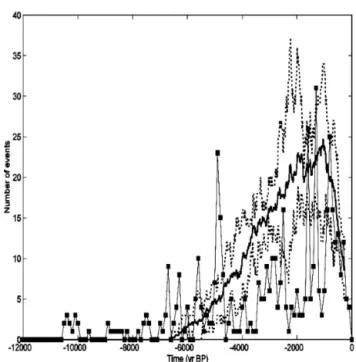
In Fig. 10 the results from the model are compared with a proxy record of ENSO from an Ecuadorian lake published by Moy et al. (2002). The proxy for ENSO is the clastic sediment washed into the lake during the heavy rains that occur almost exclusively during large El Niño events. Because the clastic sediments are so much lighter in color than the organic material

depos-ited the rest of the time, it is possible to count “events.” Figure 10 shows the number of events in 100-yr win-dows in both model and data. Model warm events are defined as years in which the December–February mean Niño-3 index exceeds 3°C. This event index cor-responds to the middle of the rainy season in coastal South America, when SST anomalies associated with large ENSO events move the ITCZ equatorward and bring large precipitation anomalies to Ecuador and Peru. An ensemble of seven experiments was per-formed to better determine which aspects of the ENSO behavior are related to the forcing and which to inter-nal variability. The agreement between the model and data implies that both the increase in number of warm events over the Holocene as well as the peak around 1000 B.P. can be explained solely by tropical Pacific coupled interactions in response to orbital forcing. Clement et al. (2000) found that the mean state change in the mid-Holocene was small but La Niña–like in that temperatures in the equatorial eastern Pacific cooled by more than those in the west.

There is a large degree of suborbital time-scale vari-ability in both the model and data. The ensemble shows that some fraction of this can be explained by variabil-ity internal to the tropical Pacific (since the model is confined to that region). However, the data variance exceeds that of the ensemble. This may be an artifact of the data recorder; it is plausible that the flux of clastic sediment due to precipitation changes has greater vari-ance than Niño-3 SST. Another possibility is that other climate forcings, not accounted for in the model experi-ment, affect ENSO behavior over the Holocene. Solar irradiance, for example, varies on time scales of de-cades to centuries (Crowley 2000), and Mann et al. (2004) have shown that ENSO behavior is sensitive to even small irradiance changes.

There are several studies with AOGCMs that cor-roborate the results of the intermediate model. Experi-ments have been done in which the orbital configura-tion was set to either 6, 9, or 11 kyr B.P. (Kitoh and Murakami 2002; Liu et al. 2000; Otto-Bliesner et al. 2003), times in which the boreal summer insolation was stronger than today. All show that the mean state change is small and La Niña–like. Otto-Bliesner (1999) and Liu et al. (2000) find that ENSO variability (as measured by the variance of the eastern equatorial Pa-cific SST) was weaker than that of modern day. The Bjerknes feedback is again fundamental to the results. In the AOGCMs, the additional solar heating in the mid-Holocene boreal summer strengthened the Asian monsoon, increasing the trade winds in the Pacific. The Bjerknes feedback, operating in the same way in the AOGCMs as in the simpler Zebiak–Cane model,

FIG. 10. Number of warm ENSO events in 100-yr windows. The black line with squares is proxy data from a lake in Ecuador (Moy et al. 2002). Warm ENSO events are defined as light colored strata in the sediment record, which reflect pluvial episodes dur-ing large El Niño (warm) events. The solid line shows the en-semble mean of seven simulations with the Zebiak–Cane model forced by the orbital variations of the last 12 000 yr. The dotted lines show the min and max values over the ensemble. Warm ENSO events are defined in the model as years in which the December–February (DJF) SST anomaly in the Niño-3 region (5°N–5°S, 90°–150°W) exceeds 3°C. This event index corresponds to the middle of the rainy season in coastal South America during which large SST anomalies associated with ENSO events are ca-pable of causing the ITCZ to move equatorward and bring large precipitation anomalies to the region.