From dataflow specification to multiprocessor partitioned time-triggered real-time implementation

(1)

HAL Id: hal-00742908

https://hal.inria.fr/hal-00742908

Submitted on 17 Oct 2012

HAL is a multi-disciplinary open access

archive for the deposit and dissemination of

sci-entific research documents, whether they are

pub-lished or not. The documents may come from

teaching and research institutions in France or

abroad, or from public or private research centers.

L’archive ouverte pluridisciplinaire HAL, est

destinée au dépôt et à la diffusion de documents

scientifiques de niveau recherche, publiés ou non,

émanant des établissements d’enseignement et de

recherche français ou étrangers, des laboratoires

publics ou privés.

From dataflow specification to multiprocessor

partitioned time-triggered real-time implementation

Thomas Carle, Dumitru Potop-Butucaru, Yves Sorel, David Lesens

To cite this version:

Thomas Carle, Dumitru Potop-Butucaru, Yves Sorel, David Lesens. From dataflow specification

to multiprocessor partitioned time-triggered real-time implementation. [Research Report] RR-8109,

INRIA. 2012. �hal-00742908�

(2)

0 2 4 9 -6 3 9 9 IS R N IN R IA /R R --8 1 0 9 --F R + E N G

RESEARCH

REPORT

N° 8109

October 2012

From dataflow

specification to

multiprocessor

partitioned

time-triggered real-time

implementation

(3)

(4)

RESEARCH CENTRE PARIS – ROCQUENCOURT

partitioned

time-triggered real-time implementation

Thomas Carle, Dumitru Potop-Butucaru, Yves Sorel, David

Lesens

∗

Project-Team AOSTE

Research Report n° 8109 — October 2012 — 19 pages

Abstract: We consider deterministic functional speciﬁcations provided by means of synchronous

data-flow models with multiple modes and multiple relative periods. These specifications are extended to include a real-time characterization defining task periods, release dates, and dead-lines. Task deadlines can be longer than the period to allow a faithful representation of complex end-to-end flow requirements. We also extend our specifications with partitioning and allocation constraints. Then, we provide algorithms for the off-line scheduling of these specifications onto partitioned time-triggered architectures à la ARINC 653. Allocation of time slots/windows to partitions can be fully or partially provided, or synthesized by our tool. Our algorithms allow the automatic allocation and scheduling onto multi-processor (distributed) systems with a global time base, taking into account communication costs. We demonstrate our technique on a model of space flight software system with strong real-time determinism requirements.

Key-words: scheduling, distributed, partitioned, multi-rate

(5)

Implantation temps-réel time-triggered partitionnée

distribuée de spécifications flots de données

Résumé : Nous considérons des spéciﬁcations fonctionnelles de type ﬂots de données synchrone

multi-périodes avec plusieurs modes d’exécution. Ces spécifications sont étendues afin d’inclure une caractérisation temps-réel définissant des dates d’arrivée et des échéances. Les échéances des tâches peuvent être plus longues que leur période pour permettre une représentation plus réaliste des contraintes de bout Ã bout complexes existant sur les flots. Nous étendons également nos spécifications pour inclure des contraintes de partitionnement et d’allocation. Nous définissons ensuite des algorithmes pour l’ordonnancement hors ligne de ces spécifications sur des architec-tures time-triggered à la ARINC 653. L’allocation des fenêtres temporelles aux partitions peut être totalement ou partiellement fournie, ou être synthétisée par notre outil. Nos algorithmes permettent l’allocation et l’ordonnancement automatique sur des architectures multi-processeurs (distribués) disposant d’une base de temps globale, en prenant en compte les coûts de commu-nication. Nous illustrons notre approche sur un modèle de logiciel de contrôle embarqué spatial comportant des contraintes de déterminisme temps-réel strictes.

(6)

1 Introduction

This paper addresses the implementation of embedded control systems with strong functional and temporal determinism requirements. The development of these systems is usually based on model-driven approaches using high-level formalisms for the speciﬁcation of functionality (Simulink,

Scade[CCM+03]) and/or real-time system architecture and non-functional requirements (AADL

[AAD], UML/Marte [uml]).

The temporal determinism requirement also means that the implementation is likely to use time-triggered architectures and execution mechanisms deﬁned in well-established standards such as TTA, FlexRay [Rus01], ARINC 653 [ARI05], or

AUTOSAR [AUT09].

The time-triggered paradigm describes sampling-based systems (as opposed to event-driven

ones) [Kop91] where sampling and execution are performed at predeﬁned points in time.1 _The

offline computation of these points under non-functional constraints of various types (real-time, temporal isolation of different criticality sub-systems, resource allocation) often complicates sys-tem development, when compared to classical event-driven syssys-tems. In return for the increased design cost, system validation and qualification are largely simplified, which explains the early adoption of time-triggered techniques in the development of safety- and mission-critical real-time systems.

Contribution. The objective and contribution of this paper is to facilitate the development of time-triggered systems by automating the allocation and scheduling steps for significant classes of functional specifications, target time-triggered architectures, and non-functional requirements. On the application side, we consider general dataflow synchronous specifications with conditional execution, multiple execution modes, and multiple relative periods. Explicitly taking into account conditional execution and execution modes during scheduling is a key point of our approach, because the offline computation of triggering dates limits flexibility at runtime. For instance, taking into account conditional execution and modes allows for better use of system resources (efficiency) and a simple modeling of reconfigurations.

On the architecture side, we consider multiprocessor distributed architectures, taking into account communication costs during automatic allocation and scheduling.

In the non-functional domain, we consider real-time, partitioning, preemptability, and allo-cation constraints. By partitioning we mean here the temporal partitioning speciﬁc to TTA, FlexRay (the static segment), and ARINC 653, which allows the static allocation of CPU or bus time slots, on a periodic basis, to various parts (known as partitions) of the application. Also known as static time division multiplexing (TDM) scheduling, these approaches further enhance the temporal determinism of a system.

We make an original use of classical real-time characteristics such as periods, release dates, and deadlines, which we adapt to our time-triggered target. In particular, the use of deadlines that are longer than the periods naturally arises. It allows a more natural real-time speciﬁcation, improved schedulability, and less context changes between partitions (which are notoriously expensive).

The application. We apply our technique on a model of spacecraft embedded control system. Spacecrafts are subject to very strict real-time requirements. The unavailability of the avionics system (and thus of the software) of a space launcher during a few milliseconds during the

1

Partially supported by the FUI8 PARSEC project.

1

As such, it generalizes classical periodic real-time scheduling concepts, by relaxing fixed release intervals into more complex repetitive patterns.

(7)

4 Thomas Carle, Dumitru Potop-Butucaru, Yves Sorel, David Lesens

atmospheric phase may indeed lead to the destruction of the launcher. From a spacecraft system point of view, the latencies are deﬁned between acquisitions of measurement by a sensor to sending of commands by an actuator. Meanwhile, the commands are established by a set of automatism algorithms (Guidance, Navigation and Control or GNC).

Traditionally, the GNC algorithms are implemented on a dedicated processor using a classical multi-tasking approach. But today, the increase of computational power provided by space processors allows suppressing this dedicated processor and distributing the GNC algorithms on the processors controlling either the sensors or the actuators. For future spacecraft (space launchers or space tranbsportation vehicles), the navigation algorithm could for instance run on the processor controlling the gyroscope, while the control algorithm could run on the processor controlling the thruster. The suppression of the dedicated processor allows power and mass saving.

The sharing of a processor by two pieces of software (one controlling for instance a gyroscope and the other one implementing the navigation algorithm) requires the use of a hypervisor ensuring the Time and Space Partitioning (or TSP), such as ARINC 653 [ARI05]. The scheduling problem is therefore as follows: End-to-end latencies are defined at spacecraft system level, along with the offsets of sensing and actuation operations. Also provided are WCET (worst case execution time) values associated to tasks. What must be computed is the time-triggered schedule of the system, including the activation times of each partition and the bus frame. Outline. The remainder of the paper is organized as follows. Section 2 reviews related work. Section 3 defines our architecture model, spending significant space on the careful definition of time-triggered and partitioned systems. Section 4 defines our task model, including functional and non-functional aspects. Sections 5, 6, and 7 cover the scheduling algorithms and experimental results. Section 8 concludes.

2 Related work

Previous work by Forget et al. [PFB+_{11] and Marouf et al. [MGS12] on the implementation of}

multi-periodic synchronous programs, as well as previous work by Blazewicz and Chetto et al. [CSB90] on the scheduling of dependent task systems have been a major source of inspiration. By comparison, our paper provides a general treatment of ARINC 653-like partitioning and of conditional execution, and a novel use of deadlines longer than periods to allow faithful real-time speciﬁcation. Our work is also close to that of Pop et al. [PEP99], the main diﬀerences being the handling of end-to-end delays and the use of fast heuristics.

Compared to previous work by Isovic and Fohler [IF09] on real-time scheduling for predictable, yet ﬂexible real-time systems, our approach does not directly cover the issue of sporadic tasks. Instead, we focus on the representation of real-time characteristics and on a very general handling of execution conditions, allowing for important ﬂexibility inside the fully predictable domain.

Compared to classical work on the on-line real-time scheduling of tasks with execution modes (cf. Baruah et al. [BCGM99]), our oﬀ-line scheduling approach comes with precise control of timing and causalities. It is therefore more interesting for us to use a task model that directly represents execution conditions. We can then use table-based scheduling algorithms that precisely determine when the same resource can be allocated at the same time to two tasks because they are never both executed.

References on time-triggered and partitioned systems, as well as scheduling of synchronous speciﬁcations will be provided in the following sections.

(8)

3 Architecture model

In this paper, we consider both single-processor architectures and bus-based multi-processor ar-chitectures with a globally time-triggered execution model and with strong temporal partitioning mechanisms. This class of architectures covers the needs of the considered case study, but also covers platforms based on the ARINC 653, TTA, and FlexRay (the static segment) standards.

Formally, for the scope of this paper, a piece of architecture is a pair

Arch_{= (B(Arch), Procs(Arch)) formed of a broadcast message-passing bus B(Arch) connecting}

a set of processors Procs(Arch) = {P1, . . . , Pn} for some n ≥ 1. We assume that the bus does

not lose, create, corrupt, duplicate or change the order of messages it transmits. Previous work by Girault et al. [GKSS03] (among others) can be used to extend this simple model (and the algorithms of this paper) to deal with fault-tolerant architectures with multiple communication lines and more complex interconnect topologies. However, for space and clarity reasons, the remainder of the paper only focuses on extending our simple model with timing, allocation, and partitioning information speciﬁc to our time-triggered approach.

3.1 Time-triggered systems

In this section we define the notion of time-triggered system used in this paper. It roughly corre-sponds to the definition of Kopetz [Kop91], and is a sub-case of the definition of Henzinger and Kirsch [HK07]. We shall introduce its elements progressively, explaining what the consequences are in practice.

3.1.1 General definition

By time-triggered systems we understand systems satisfying the following 3 properties:

TT1 A system-wide time reference exists, with good-enough precision and accuracy. We shall refer to this time reference as the global clock. For single-processor systems the global clock

can be the CPU clock itself.2

TT2 The execution duration of code driven by interrupts other than the timers is negligible. In other words, for timing analysis purposes, code execution is only triggered by timers synchronized on the global clock.

TT3 System inputs are only read/sampled at timer triggering points.

At the same time, we place no constraint on the sequential code triggered by timers. In particular: • Classical sequential control ﬂow structures such as sequence or conditional execution are

permitted, allowing the representation of modes and mode changes. • Timers are allowed to preempt the execution of previously-started code.

This definition of time-triggered systems is fairly general. It covers single-processor systems that can be represented with time-triggered e-code programs, as they are defined by Henzinger and Kirsch [HK07]. It also covers multiprocessor extensions of this model, as defined by Fischmeister et al. [FSL06] and used by Potop et al. [PBAF10]. In particular, our model covers time-triggered communication infrastructures such as TTA and FlexRay (static and dynamic segments) [KB03, Rus01], the periodic schedule tables of AUTOSAR OS [AUT09], as well as systems following a

2

For distributed multiprocessor systems, we assume it is provided by a platform such as TTA [KB03] or by a clock synchronization technique such as the one of Potop et al. [PBAF10].

(9)

preemptive multi-processor periodic scheduling model without jitter and drift.3 _{It also covers}

the execution mechanisms of the avionics ARINC 653 standard [ARI05] provided that interrupt-driven data acquisitions, which are conﬁned to the ARINC 653 kernel, are presented to the application software in a time-triggered fashion satisfying property TT3. To our knowledge, this constraint is satisﬁed in all industrial settings.

3.1.2 Model restriction

The major advantage of time-triggered systems, as deﬁned above, is that they have the property

of repeatable timing [EKL+_{09]: For any two input sequences that are identical in the large-grain}

timing scale determined by the timers of a program, the behaviors of the program, including

timing aspects, are identical.4

This property is extremely valuable in practice because it largely simpliﬁes debugging and testing of real-time programs. A time-triggered platform also insulates the developer from most problems stemming from interrupt asynchrony and low-level timing aspects.

However, the applications we consider have even stronger timing requirements, and must

satisfy a property known as timing predictability [EKL+_{09]. Ideally, formal timing guarantees}

should be provided by means of oﬀ-line (static) analysis. The general time-triggered model deﬁned above remains too complex to allow the analysis of real-life systems. To facilitate analysis, this model is usually restricted and used in conjunction with worst-case execution time guarantees on the sequential code fragments.

In this paper we consider a restriction of the general deﬁnition provided above where timer triggers occur following a ﬁxed pattern which is repeated periodically in time. Following the convention of ARINC 653, we call this period the major time frame (MTF). The timer triggering

pattern is provided under the form of a set of fixed offsets 0 ≤ t1< t2< . . . < tn<MTF defined

with respect to the start of each MTF period. Note that the code triggered at each oﬀset may still involve complex control, such as conditional execution or preemption.

This restriction corresponds to the classical definition of time-triggered systems by Kopetz [Kop91, KB03]. It covers our target platform, TTA, FlexRay (the static segment), and AU-TOSAR OS (the periodic schedule tables). At the same time, it does not fully cover ARINC 653. As defined by this standard, partition scheduling is time-triggered. The strict temporal partitioning also implies that all input/output is sampled, and that code execution is triggered by timers [MLL06]. However, given that periodic processes can be started (in normal mode) with a release date equal to the current time (not a predefined date), intra-partition process scheduling does not fit our restricted model. To do so, an ARINC 653 system should not start periodic processes after system initialization, i.e. in normal mode.

3.2 Temporal partitioning

Our target architectures follow a strong temporal partitioning paradigm similar to that of ARINC

653.5 _{In this paradigm, both system software and platform resources are statically divided among}

a ﬁnite set of partitions Part = {part1, . . . ,partk}. Intuitively, a partition comprises both a

software application of the system and the execution and communication resources allocated to

it.6

3

But these two notions must be accounted for in the construction of the global clock [PBAF10].

4

We assumed that programs are functionally deterministic.

5

Spatial partitioning aspects are not covered in this paper.

6

The aim of this static allocation is to limit the functional and temporal influence of one partition on another to a set of explictly-specified inter-partition communication and synchronization mechanisms.

(10)

We are mainly concerned in this paper with the execution resource represented by the pro-cessors. To eliminate timing interference between partitions, the static partitioning of processor time between the partitions running on it is done by means of a static time division multiplexing (TDM) scheme. In our case, the TDM scheme is built on top of the time-triggered model of

the previous section. It is implemented by partitioning, separately for each processor Pi, the

MTF deﬁned above into a ﬁnite set of non-overlapping windows Wi = {wi1, . . . , wkii} having each

a ﬁxed start oﬀset twi

j and duration dwij. Each window is then allocated to a single partition

partwi

j, or left unused. Unused windows are called spares and identiﬁed by partwij = spare.

Software belonging to partition part_ican only be executed during windows belonging to part_i.

Unﬁnished partition code will be preempted at window end, to be resumed at the next window of the partition. There is an implicit assumption that the scheduling of operations inside the MTF will ensure that non-preemptive operations will not cross window end points.

For the scheduling algorithms of Section 6, the partitioning of the MTF into windows can be either an input or an output. More precisely, all, none, or part of the windows can be provided as input to the scheduling algorithms.

4 Task model

Following classical industrial design practices, the specification of our scheduling problem is formed of a functional specification and a set of non-functional properties. Represented in an abstract fashion, these two components form what is classically known as a task model used in the definition of our scheduling algorithms. In our case, the functional specification is provided under the form of a set of dependent tasks with a cyclic execution model. Non-functional properties include the real-time task characteristics, the allocation constraints, the preemptability of the tasks, and the partitioning constraints.

4.1 Functional specification

4.1.1 Simplifying assumptions

Our scheduling technique works on functional speciﬁcations of dataﬂow synchronous type. This allows the faithful representation of dependent task systems featuring multiple execution modes, conditional execution, and multiple relative periods.

However, the presentation of the scheduling results of this paper does not require a full description of all the details of this formalism. The task model we formally define abstracts away two difficult aspects of synchronous modeling and analysis. We present them here, pointing the reader to detailed papers covering the topics and explaining why the simplification does not reduce the generality of our results.

The ﬁrst simplifying assumption concerns the relative periods of tasks. Assume that our

scheduling problem requires tasks τ and τ′ _{to have periods of 5 ms (milliseconds) and 20 ms,}

respectively. In this requirement, the real-time information is a non-functional property, deﬁned

later. But the ratio between the periods of τ and τ′ belongs to the functional speciﬁcation,

facilitating for instance the deﬁnition of the way τ and τ′ _{exchange data by means of a ﬁnite}

pattern which is repeated periodically.

Our simplifying assumption is that we work on single-period task systems where the period ratio is always 1. This simplification does not affect generality, because multi-period specifications can always be transformed into single-period ones by means of a hyper-period expansion. For

instance, the hyperperiod of tasks τ and τ′ _{is 20 ms. The hyperperiod expansion consists in}

(11)

by 4 tasks τ1, τ2, τ3, and τ4, all of period 20ms. Task τ′ does not require replication because its

period is 20 ms. Section 4.1.3 will provide a larger modeling example.

The compact representation of the functional part of multi-period speciﬁcations, as well as

its efficient manipulation for scheduling purposes is elegantly covered by Forget et al. [PFB+_11],

drawing inﬂuences from Chetto et al. [CSB90] and Pouzet et al. [CDE+_{06], among others.}

The second simplification concerns execution modes and conditional execution. Our model represents this information in an abstract way, by means of an exclusion relation between task instances. A full-fledged definition and analysis of the data expressions used as execution condi-tions has been presented elsewhere [PBAF10] and would take precious space in this paper.

4.1.2 Dependent task systems

The previous simplifications allow us to use the following model of dependent task system, which we define in 2 steps. The first covers systems with a single execution mode:

Definition 1 (Non-conditioned dependent task set) A non-conditioned dependent task sys-tem is a directed graph defined as a triple D = {T (D), A(D), ∆(D)}. Here, T (D) is the finite set of tasks. The finite set A(D) contains typed dependencies of the form a = (src(a), dst(a), type(a)), where src(a), dst(a) ∈ T (D) are the source, respectively the destination task of a, and type(a) is its type (identified by a name). The directed graph determined by A(D) must be acyclic. The finite set ∆(D) contains delayed dependencies of the form δ = (src(δ), dst(δ), type(δ), depth(δ)), where src(δ), dst(δ), type(δ) have the same meaning as for regular dependencies and depth(δ) is a strictly positive integer.

Non-conditioned dependent task sets have a cyclic execution model. At each execution cycle

of the task set, each of the tasks is executed exactly once. We denote with tn _{the instance of}

task t ∈ T (D) for cycle n. The execution of the tasks inside a cycle is partially ordered by the

dependencies of A(D). If a ∈ A(D) then the execution of src(a)n _{must be ﬁnished before the}

start of dst(a)n_{, for all n. Note that dependency types are explicitly deﬁned, allowing us to}

manipulate communication mapping.

The dependencies of ∆(D) impose an order between tasks of successive execution cycles. If

δ∈ ∆(D) then the execution of src(δ)nmust complete before the start of dst(δ)n+depth(δ)_{, for all}

n.

We are now ready to provide the full deﬁnition covering speciﬁcations with multiple execution modes.

Definition 2 (Dependent task set) A dependent task set is a tuple

D = {T (D), A(D), ∆(D), EX(D)} where {T (D), A(D), ∆(D)} is an unconditioned dependent

task set and EX(D) is an exclusion relation EX(D) ⊆ T (D) × T (D) × N.

The introduction of the exclusion relation modiﬁes the execution model deﬁned above as follows:

if (τ1, τ2, k) ∈ EX(D) then τ1n and τ2n+k are never both executed, for any execution of the

modeled system and any cycle index n. For instance, if the activations of τ1 and τ2 are on

the two branches of a test we will have (τ1, τ2,0) ∈ EX(D). The relation EX(D) needs not be

computed exactly (it can even be void) but the more precise it is, the better results the scheduling algorithms will give because tasks in an exclusion relation can be allocated the same resources at the same dates.

4.1.3 Modeling of the case study

The specification of the space flight application mentioned in the introduction was provided under the form of a set of AADL [AAD] diagrams, plus textual information defining specific

(12)

inter-task communication patterns, determinism requirements, and a description of the target hardware architecture. We present here its simpler version (with fewer tasks), the results on the full example being provided in Section 7.

Our first step was to derive a task model in our formalism. In doing this we discovered that the initial system was over-specified, in the sense that real-time constraints were imposed in order to ensure causal ordering of tasks instances using AADL constructs. Removing these constraints gave us more freedom for scheduling, allowing for a reduction in the number of partition changes. The resulting specification is presented in Fig. 1.

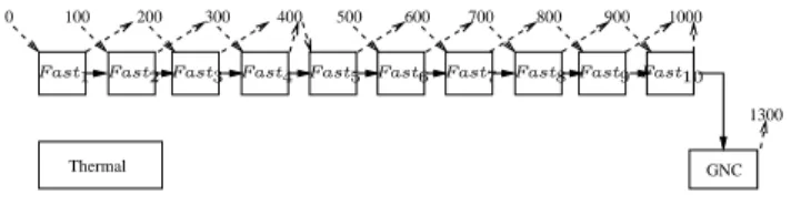
GNC Thermal

0 100 200 300 400 500 600 700 800 900

Fast2

Fast1 Fast3 Fast4 Fast5 Fast6 Fast7 Fast8 Fast9 Fast10

δ

Figure 1: The Simple example (MTF=1000 time units)

Our model, named Simple represents a system with 3 tasks Fast, GNC, and Thermal. The periods of the 3 tasks are 100, 1000, and 1000 time units, respectively, meaning that Fast is executed 10 times for each execution of GNC and Thermal. The hyper-period unfolding described

in Section 4.1.1 replicates task Fast 10 times, the resulting tasks being Fasti, 1 ≤ i ≤ 10.

Tasks GNC and Thermal are left unchanged. The direct arcs connecting the tasks Fasti and

GNC represent regular (intra-cycle) data dependencies of A(Simple). The arcs labeled with δ are delayed data dependencies of depth 1 where information is transmitted from one execution cycle of the synchronous speciﬁcation to the next. In this simple model, task Thermal has no dependencies. Dashed arcs and numerical values are the real-time characterization of the model, explained in the next section.

Representing execution modes. Our first model has no execution modes. However, the input specification allows the specification of modes under the form of mode-dependent durations for the various tasks. There is also a requirement that task start dates (after scheduling) do not change with the mode. This is consistent with the practice of grouping into each task several functions that can be turned on or off individually according to the execution mode. We explain below how our task model allows the representation of such specifications. Note, however, that our algorithms could take better advantage of a specification where each function is associated an individual task, providing more degrees of freedom to the scheduler.

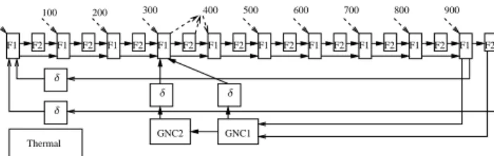
GNC1 Thermal F1 F1 F1 F1 F1 F1 F1 F1 F1 F1 GNC2 900 700 600 800 500 400 300 0 100 200 F2 F2 F2 F2 F2 F2 F2 F2 F2 F2 δ δ δ δ

Figure 2: Representing mode-dependent WCET variations

(13)

ﬂight modes), each of the tasks Fast and GNC having a diﬀerent duration in each of the modes.

We denote these durations respectively with WCET(Fast, P )mode and WCET(GNC, P )mode for

mode = 1, 2 and P ranging over the processors where the two tasks can be executed. We assume

that WCET(Fast, P )1<WCET(Fast, P )2and that WCET(GNC, P )1>WCET(GNC, P )2for all

P(a form of monotony). Then, our modeling is based on the use of 2 tasks for the representation

of each of Fast and GNC. The ﬁrst task represents the part of computation of shorter duration, whereas the second task represents the remainder, which is only needed in modes where the duration is longer. Note that more than 2 tasks are needed when a task can have 3 or more diﬀerent durations. The resulting model is pictured in Fig. 2. Here, Fast has been split into F1 and F2, the second one being executed only in mode 2. GNC has been split into GNC1 and GNC2, the second one being executed only in mode 1. We assume the mode change is triggered

such that (GNC2, F2i,1) ∈ EX(Simple) for 1 ≤ i ≤ 10, which will allow GNC2 and the tasks

F2i to partially overlap if they are placed in the same partition.

4.2 Non-functional properties

Our task model considers non-functional properties of real-time, allocation, and partitioning types.

4.2.1 Period, release dates, and deadlines

The functional speciﬁcation of the previous section is usually provided by the control engineers, which must also provide a real-time characterization in terms of periods, release dates, and

deadlines.7 _{More constraints of the same types may be imposed by the system architecture, as}

explained below. Our model allows the specification of these characteristics in a specific form adapted to our functional specification model and time-triggered implementation paradigm. Period. Recall from the previous section that after hyper-period expansion all the tasks of a dependent task system D have same period. In the functional model, each task is executed once per execution cycle, modulo conditional execution modeled by relation EX(D). Defining the period of these tasks is easily done by defining the period with which execution cycles are started. We shall call this period the major time frame of D and denote it MTF(D). We will require it to be equal to the MTF of its time-triggered implementation, as defined in Section 3.1.2. Throughout this paper, we will assume that MTF(D) is an input to our scheduling problem. Other scheduling heuristics, more directly derived from those of [PBAF10] can be used in the case where it must be computed.

Release dates and deadlines. For each task τ ∈ T (D), we allow the definition of a release date r(τ) and a deadline d(τ). Both are positive offsets defined with respect to the start date of the current cycle. Their default values, meaning that no constraint is imposed, are respectively 0 and ∞.

This definition is consistent with our time-triggered implementation target where all inputs are sampled. The main assumption we make is that the sampling offsets are an input to our scheduling problem, specified using the release dates defined above.

End-to-end latency requirements are specified using a combination of both release dates and deadlines. Indeed, such end-to-end latencies should be defined on flows (chains of dependent task instances) starting with an input acquisition and ending with an output. Since acquisitions

7

This characterization is directly derived from the analysis of the control system, and does not depend on architecture details such as number of processors, speed, etc.

(14)

have fixed positions, the latency constraints can also be specified using fixed offsets, namely the deadlines.

Even though the release dates and deadlines defined above have the same meaning as in classical real-time, there is a fundamental difference: In our implementations the scheduler never uses these values directly (they are specification objects), relying instead on the start dates computed offline.

Modeling of the case study. The speciﬁcation in Fig. 1 has MTF(Simple) = 1000 time units. Release dates and deadlines are respectively represented using descending and mounting dashed arcs. The release dates specify that task Fast uses an input that is sampled with a period of 100

time units, starting at date 0, which imposes a release date of n ∗ 100 for the nth _{instance of task}

Fast. Although, by transitivity, the release dates on Fast constrain the start of GNC, we do not consider these constraints to be a part of the speciﬁcation itself. Thus, we set the release dates of tasks GNC and Thermal to the default value 0 and do not represent them graphically.

Only task Fast4has a deadline that is diﬀerent from the default ∞ (and is thus represented).

In conjunction with the 0 release date on Fast1, this deadline represents an end-to-end constraint

of 1400 time units on the flow deﬁned by the chain of task instances Fast1n→ Fast2n → . . . →

Fast10n → GNCn → Fast4n+1 for n ≥ 0. The deadline on Fast4 is of 400 time units, and not

1400, because the flow covers two successive execution cycles of our functional specification. The end of the flow belonging to the second execution cycle, we must subtract one MTF (1000 in our case) from the end-to-end constraint value (1400 time units).

The release dates and deadlines of Fig. 1 represent architectuindependent real-time re-quirements that must be provided by the control engineer. But architecture details may impose constraints of their own. For instance, assume that the samples used by task Fast are stored in a 3-place circular buﬀer. At each given time, Fast uses one place for input, while the hardware

uses another to store the next sample. Then, to avoid buﬀer overrun, the computation of Fastn

must be completed before date (n + 1) ∗ 100, as required by the new deadlines of Fig. 3. Note

that these deadlines can be both larger than the period of task Fast, and larger than the MTF

(for Fast10) to allow the faithful representation of our real-time constraints. By comparison, the

specification of Fig. 1 corresponds to the assumption that input buffers are infinite.

GNC Thermal

0 100 200 300 400 500 600 700 800 900 1000 1100

Fast2

δ

Figure 3: Adding 3-place circular buﬀer constraints to our example

4.2.2 Worst-case durations, allocations, preemptability

We also need to describe the processing capabilities of the various processors and the bus. More precisely:

• For each task τ ∈ T (D) and each processor P ∈ Procs(Arch) we provide the capacity, or duration of τ on P . We assume this value is obtained through a worst-case execution time (WCET) analysis, and denote it WCET(τ, P ). This value is set to ∞ when execution of τ on P is not possible.

(15)

• Similarly, for each data type type(a) used in the speciﬁcation, we provide WCCT(type(a)) as an upper bound on the transmission time of a value of type type(a) over the bus. We assume this value is always ﬁnite.

Note that the WCET information may implicitly deﬁne absolute allocation constraints, as WCET(t, P ) = ∞ prevents t from being allocated on P . Such allocation constraints are meant to represent hardware platform constraints, such as the positioning of sensors and actuators, or designer-imposed placement constraints. Relative allocation constraints can also be deﬁned, under the form of task groups which are subsets of T (D). The tasks of a task group must be allocated on the same processor. The use of task groups is necessary in the representation of mode-dependent task durations, as presented in Section 4.1.3 (to avoid task migrations). It is also needed in the transformations of Section 5.

Our task model allows the representation of both preemptive and non-preemptive tasks. The preemptability information is represented for each task τ by the ﬂag is_preemptive(τ). We assume that bus communications are non-interruptible. Throughout this paper we make the

simplifying assumption that preemption and partition context switch costs are negligible.8

4.2.3 Partitioning

Recall from Section 3.2 that there are two aspects to partitioning: the partitioning of the applica-tion and that of the resources (in our case, CPU time). On the applicaapplica-tion part, we assume that

every task τ is associated to a partition part_τ of a ﬁxed partition set Part = {part1, . . . ,partk}.

Also recall from Section 3.2 that CPU time partitioning, i.e the time windows on processors and their allocation to partitions can be either provided as part of the specification or computed by our algorithms. Thus, our specification may include window definitions which cover none, part, or all of CPU time of the processors. We do not specify a partitioning of the shared bus, but the algorithms can be easily extended to support a per-processor time partitioning like that of TTA [Rus01].

5 Removal of delayed dependencies

The first step in our scheduling approach is the transformation of the initial task model spec-ification into one having no delayed dependency. This is done by a modspec-ification of the release dates and deadlines for the tasks related by delayed dependencies, possibly accompanied by the creation of new helper tasks that require no resources but impose scheduling constraints. Doing this will allow in the next section the use of simpler scheduling algorithms that work on acyclic task graphs.

The ﬁrst part of our transformation ensures that delayed dependencies only exist between tasks that will be scheduled on the same processor. Assume that δ ∈ ∆(D) and src(δ) and dst(δ) are not forced by absolute or relative allocation constraints to execute on the same processor.

Then, we add a new task τδ _{to D. The source of δ is reassigned to be τ}δ_{, and a new}

(non-delayed) dependency is created between src(δ) and τδ_{. Relation EX(D) is augmented to place}

τδ _{in exclusion with all tasks that are exclusive with src(δ). Task τ}δ _{is assigned durations of 0 on}

all processors where dst(δ) can be executed, and ∞ elsewhere. Finally, a task group is created

containing τδ _{and dst(δ).}

The second part of our transformation removes the delayed dependencies. It does so by imposing for each delayed dependency δ that src(δ) terminates its execution before the release

8

Taking them into account is work in progress

(16)

GNC Thermal 100 200 300 400 500 600 700 800 900 1000 1300 0 Fast2

Figure 4: Delay removal result

date of dst(δ). This is done by changing the deadline of src(δ) to r(dst(δ)) + depth(δ) ∗ MTF(D) whenever this value is smaller than the old deadline.

Finally, task deadlines are changed following the approach of Blazewicz, as cited by Chetto et al. [CSB90]. More precisely, the deadline of each task is set to be the minimum of all deadlines

of tasks depending transitively on it (including itself).9

The result of all these transformations for the example in Fig. 3, assuming that tasks Fast4

and GNC are always allocated on the same processor and thus no helper task is needed, is pictured in Fig. 4. Note that this transformation is another source of deadlines larger than the periods. Also note that all the transformations described above are linear in the size of the number of arcs (delayed or not), and thus very fast.

6 Offline real-time scheduling

On the transformed task models we apply an offline scheduling algorithm whose output is a system-wide scheduling table deﬁning the allocation of processor and bus time to the various computations and communications. The length of this table is equal to the MTF of the task model.

Our oﬄine scheduling algorithm is a signiﬁcant extension of those described by Potop et al. [PBSST09]. New features are the handling of preemptive tasks, release dates and deadlines, the MTF, and the partitioning constraints. Other major features remain largely unchanged. This is the case for the handling of conditional execution and bus communications. We do not present these features in detail, instead pointing the interested reader to reference [PBSST09]. Instead, we insist on the novelty points, like the deadline-driven scheduler inspired by existing work by Blazewicz (cited by Chetto et al. [CSB90]).

6.1 Basic principles

As earlier explained, our algorithm computes a scheduling table. This is done by associating to each task a target processor on which it will execute, a set of time intervals that will be reserved for its execution, and a date of first start. The conditional execution paradigm of our task model implies the use of conditional reservations: The same time interval can be reserved to two or more tasks if they are mutually exclusive, as deﬁned by relation EX(D). A similar reservation model is used for the bus [PBSST09].

Given a scheduling table S of task system D, and τ ∈ T (D), we shall denote with S.proc(τ) the target processor of τ, with S.start(τ) the date of ﬁrst start, and with S.intervals(τ) the set of time intervals reserved for τ. A time interval i is deﬁned by its start date start(i) and end date end(i). It is required that the intervals of S.intervals(τ) are disjoint, and that the start date of

9

More generally, the recomputation of release dates and deadlines by means of a fixed-point computation can be useful before the removal of delayed arcs to provide for longer deadlines.

(17)

one of them is

S.start(τ) mod MTF(D).

The execution model is as follows: The nth _{instance of task τ will start (modulo conditional}

execution) at date S.start(τ) + n ∗ MTF(D). If its execution terminates before consuming all reserved intervals, unused space can be used by any of the suspended tasks belonging to the same partition as τ (arbitrating between multiple such tasks can be done using a priority-driven scheme not covered here). A task is suspended between intervals reserved for itself, unless using free space from another task.

The choice of processor, start date, and intervals by the scheduling algorithm must ensure that:

• The intervals reserved for a task allow the complete execution of a task instance before the next instance is started.

• Intervals of two tasks can only overlap if the two tasks are exclusive.

• The task and communication execution order imposed by the direct and delayed depen-dencies is respected.

• The release date of a task precedes its start date, and deadline constraints are respected. • Intervals reserved for two tasks of diﬀerent partitions cannot overlap. Moreover, an interval

allocated to task τ of a partition part cannot overlap with windows allocated to other partitions.

6.2 Scheduling algorithms

The scheduling algorithm, whose top-level routine is Procedure 1, follows a classical list schedul-ing approach. It works by iteratively choosschedul-ing a new task to schedule and then schedulschedul-ing it and the necessary communications.

Among the not-yet-scheduled tasks of whom all predecessors have been executed, function choose_task_to_schedule, not provided here, returns the one of minimal deadline. If several tasks satisfy this criterion, it returns one of greatest release date.

The body of the while loop allocates and schedules a single task τ, along with the commu-nications needed to gather the input data of τ. It works by attempting to schedule τ on each of the processors that can execute it. Function group_ok determines if the relative allocation constraints and the current scheduling state allow τ to be allocated on P .

Among all the possible allocations of τ, Procedure 1 chooses the one resulting in a schedule of minimal cost. In our case, cost_function chooses the schedule ensuring the earliest termination of τ. If scheduling is not possible on any of the processors Procedure 1 returns invalid_ schedule to identify the failure.

Procedure 2 does the actual scheduling of a task τ on a processor P , following a classical ASAP (as soon as possible) scheduling strategy. The scheduling is done as follows. First, the transmission of data needed by τ and not yet present on P is scheduled for communication on the bus using function schedule_bus_communications. This function schedules the transmission of both input data of τ and state variables needed to compute the execution condition of τ. We do not provide the function here, interested readers being directed to [PBSST09].

Once communications are scheduled, we attempt to schedule the task at the earliest date after the date where all needed data is available. If this is not possible without missing the deadline, invalid_scheduling is returned to identify the failure. To allow an eﬃcient search for free time intervals, the data structure storing the partial schedules also stores the set of free intervals of

(18)

Procedure 1 scheduler_driver

Input: D : dependent task system

Arch: architecture description

initial_schedule : schedule Output: result : system schedule

result:= initial_schedule

while T (D) 6= ∅ and result 6= invalid_schedule do τ:= choose_task_to_schedule(D)

new_schedule := invalid_schedule

new_cost :=∞

for all P in Archi do

if WCET(τ, P ) 6= ∞ and group_ok(τ,P ,result) then temp_sched :=

schedule_task_on_proc(τ,P,result,MTF) temp_cost := cost_function(temp_sched ) if temp_cost < new_cost then

new_schedule := temp_sched new_cost := temp_cost

result:= new_schedule

T(D) := remove_task(τ, T (D))

the processors and buses. Window allocations taken as input by our scheduler are passed to Procedure 1 through parameter initial_schedule, which contains no task allocation, but already constrains the free interval set.

Looking for individual intervals is done by function get_first_interval, not provided here. This function takes as input the preemptability flag of the task. For non-preemptive tasks, it looks for the first free interval long enough to allow the execution of the task and satisfying the execution condition and partitioning constraints. For preemptive tasks, this function may be called several times to find the first free intervals satisfying the execution condition and partitioning constraints and of sufficient cummulated length to cover the needed duration. When unable to find a valid interval, function get_first_interval returns an invalid interval identifying the failure. Depending on the task deadline, the search for free intervals may loop over the MTF.

7 Post-scheduling slot minimization

The algorithm of the previous section follows a classical ASAP deadline-driven scheduling policy. Such policies are good at ensuring schedulability. It is easy to prove that our algorithm is even optimal in certain cases (all-preemptive, single processor, no execution condition, no delayed dependency).

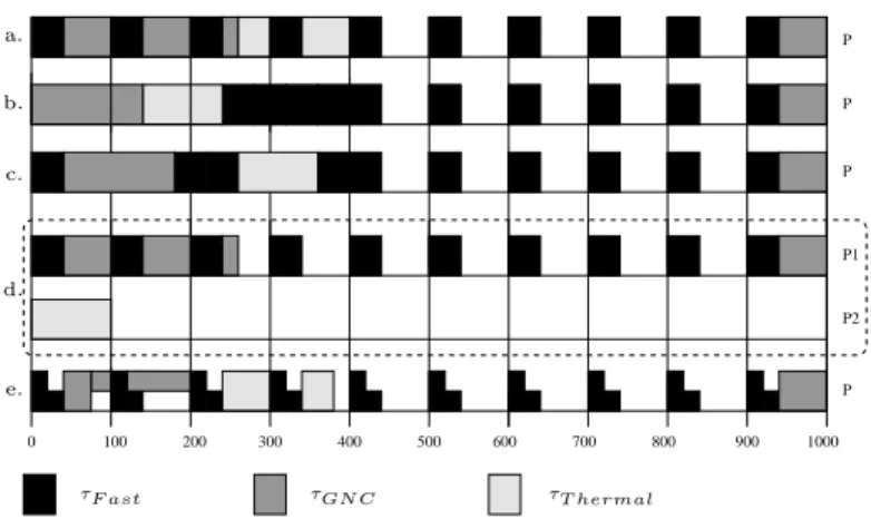
However, resulting schedules may have a lot of unneeded preemptions and, most importantly, partition changes which are notoriously expensive. Consider our example of Fig. 1 and an architecture with a single processor P such that WCET(Fast, P ) = 40, WCET(GNC, P ) = 140, and WCET(Thermal, P ) = 100. We assume a partitioning approach à la IMA, where the 3 tasks have each one partition. Then, Fig. 5(a) provides the output of the scheduling phase. This ﬁgure shows the allocation of the time intervals to the various tasks over the MTF. Time ﬂows from left to right, and the target processor is shown on the right. This schedule features no less than

(19)

Procedure 2 schedule_task_on_proc

Input: τ : task to schedule

P: processor on which to schedule

schedule: scheduling state before adding τ

MTF : major time frame of the task system Output: result : schedule after adding τ

result:= schedule (result, dearliest) := schedule_bus_communications(τ, P, result) if dearliest> d(τ)then result:= invalid_schedule else needed_duration := WCET(τ, P) interval_set :=∅ failure := false

while needed_duration > 0 and not failure do (interval, result.free_interval_set):=

get_first_interval(result.free_interval_set,

needed_duration, d(τ), dearliest,

partτ,is_preemptive(τ))

if is_valid(interval) then

interval_set := interval_set∪ {interval}

dearliest:=end(interval) needed_length:=needed_length-len(interval) else if deadline ≤ MTF then failure := true else deadline:=deadline-MTF(D) dearliest:=0 if failure then result:= invalid_schedule else result:= set_task_intervals(result,τ,interval_set) Inria

(20)

P P P P P1 P2 300 400 500 600 700 800 900 1000 0 100 200 τF ast τGN C τT hermal c. a. b. d. e.

Figure 5: Resulting schedules: For the example in Fig. 1, single-processor without slot mini-mization (a) and with it (b), and bi-processor (d). For the example in Fig. 3 (c), and for the two-mode example of Fig. 2 (e).

end of Fast10).

To mitigate this issue, we perform a heuristic post-scheduling schedule transformation aimed at reducing partition changes. The transformation we apply is the following: The scheduling

table is traversed from end to the beginning. Whenever two intervals i1and i2allocated to tasks

of the same partition are separated by intervals of another partition, we attempt to group i1

and i2 together. Assuming i1 starts before i2, our technique attempts to move i1just before i2

while moving all operations between i1 and i2 to earlier dates. The transformation step is only

performed when the resulting schedule respects the correctes properties of Section 6.1.

The result of the transformation on our example is provided in Fig. 5(b) (only 3 partition changes). Fig. 5(c) provides the schedule obtained for the more constrained example in Fig. 3.

We also provide in Fig. 5(d) an example of bi-processor scheduling (there are no bus commu-nications to represent), and the scheduling of the two-mode speciﬁcation of Fig. 2, in Fig. 5(e)). In this last case, we assume that tasks F2 and GNC belong to the same partition. Notice that the second instance of F2 and GNC share a reservation.

A larger example We have implemented our scheduling algorithms into a tool, which allowed us to schedule the proof-of-concept versions of the target application, as presented above. More important, we have been able to build and schedule a large-scale model of the application, involving 4 processors, 13 tasks, and 8 end-to-end ﬂow constraints. We do not present it here for space reasons.

8 Conclusion and future work

We have proposed a technique for the distributed partitioned time-triggered implementation of synchronous dataﬂow speciﬁcations featuring multiple periods and conditional execution (and modes). Implementation can be done under end-to-end latency and partitioning constraints. We have successfully applied our technique on a realistic spacecraft case study.

Future work will focus on 2 main directions. On the scheduling side, we will focus on the ﬁne tuning of the scheduling and the promising slot minimization heuristics. On the modeling

(21)

side, we will take inspiration from Forget et al. to allow the compact representation and eﬃcient manipulation of multi-period task models. It is important here to preserve a faithful represen-tation of timing requirements, without over-constraining, and to allow a smooth integration of conditional execution.

References

[AAD] The AADL formalism page: http://www.aadl.info/.

[ARI05] ARINC 653: Avionics application software standard interface. www.arinc.org, 2005.

[AUT09] Autosar (automotive open system architecture), release 4.

http://www.autosar.org/, 2009.

[BCGM99] S. Baruah, D. Chen, S. Gorinsky, and A. Mok. Generalized multiframe tasks. Real-Time Systems, 17(1), July 1999.

[CCM+_{03] P. Caspi, A. Curic, A. Magnan, C. Sofronis, S. Tripakis, and P. Niebert. From}

Simulink to SCADE/Lustre to TTA: a layered approach for distributed embedded applications. In Proceedings LCTES, San Diego, CA, USA, June 2003.

[CDE+_{06] A. Cohen, M. Duranton, C. Eisenbeis, C. Pagetti, F. Plateau, and M. Pouzet.}

N-synchronous kahn networks: a relaxed model of synchrony for real-time systems. In POPL, pages 180–193, 2006.

[CSB90] H. Chetto, M. Silly, and T. Bouchentouf. Dynamic scheduling of real-time tasks

under precedence constraints. Real-Time Systems, 2, 1990.

[EKL+_{09] S.A. Edwards, S. Kim, E.A. Lee, I. Liu, H.D. Patel, and M. Schoeberl. A disruptive}

computer design idea: Architectures with repeatable timing. In Proceedings ICCD. IEEE, October 2009. Lake Tahoe, CA.

[FSL06] S. Fischmeister, O. Sokolsky, and I. Lee. Network-code machine: Programmable

real-time communication schedules. In Proceedings RTAS 2006., april 2006.

[GKSS03] A. Girault, H. Kalla, M. Sighireanu, and Y. Sorel. An algorithm for automatically obtaining distributed and fault-tolerant static schedules. In Proceedings DSN, San Francisco, CA, USA, 2003.

[HK07] T.A. Henzinger and C. Kirsch. The embedded machine: Predictable, portable

real-time code. ACM Transactions on Programming Languages and Systems, 29(6), Oct 2007.

[IF09] D. Isovic and G. Fohler. Handling mixed sets of tasks in combined oﬄine and online

scheduled real-time systems. Real-Time Systems, 43:296–325, 2009.

[KB03] H. Kopetz and G. Bauer. The time-triggered architecture. Proceedings of the IEEE,

91(1):112–126, 2003.

[Kop91] H. Kopetz. Event-triggered versus time-triggered real-time systems. In LNCS 563,

volume 563 of Lecture Notes in Computer Science, pages 87–101, 1991.

(22)

[MGS12] M. Marouf, L. George, and Y. Sorel. Schedulability analysis for a combination of non-preemptive strict periodic tasks and preemptive sporadic tasks. In Proceedings ETFA’12, Kraków, Poland, September 2012.

[MLL06] J.F. Mason, K. R. Luecke, and J.A. Luke. Device drivers in time and space

partitioned operating systems. In 25th Digital Avionics Systems Conference,

IEEE/AIAA, Portland, OR, USA, Oct. 2006.

[PBAF10] D. Potop-Butucaru, A. Azim, and S. Fischmeister. Semantics-preserving implemen-tation of synchronous speciﬁcations over dynamic TDMA distributed architectures. In Proceedings EMSOFT, Scottsdale, Arizona, USA, 2010.

[PBSST09] D. Potop-Butucaru, R. De Simone, Y. Sorel, and J.-P. Talpin. Clock-driven dis-tributed real-time implementation of endochronous synchronous programs. In Pro-ceedings EMSOFT’09, pages 147–156, 2009.

[PEP99] P. Pop, P. Eles, and Z. Peng. Scheduling with optimized communication for

time-triggered embedded systems. In Proceedings CODES’99, 1999.

[PFB+_{11] C. Pagetti, J. Forget, F. Boniol, M. Cordovilla, and D. Lesens. Multi-task}

implemen-tation of multi-periodic synchronous programs. Discrete Event Dynamic Systems, 21(3):307–338, 2011.

[Rus01] J. Rushby. Bus architectures for safety-critical embedded systems. In Proceedings

EMSOFT’01, volume 2211 of LNCS, Tahoe City, CA, USA, 2001.

(23)

RESEARCH CENTRE PARIS – ROCQUENCOURT

Domaine de Voluceau, - Rocquencourt B.P. 105 - 78153 Le Chesnay Cedex

Publisher Inria

Domaine de Voluceau - Rocquencourt BP 105 - 78153 Le Chesnay Cedex inria.fr