Data-Driven Revenue Management
by
Joline Ann Villaranda Uichanco
Submitted to the School of Engineering
in partial fulfillment of the requirements for the degree of
Master of Science in Computation for Design and Optimization
at the
MASSACHUSETTS INSTITUTE OF TECHNOLOGY
September 2007
©
Massachusetts Institute of Technology 2007. All rights reserved.
A uthor ...
... :...
IU
hc ool of Engineering September 17, 2007Certified by... ...
.. ...
J
Retsef Levi
Robert N. Noyce Career Development Professor, Assistant Professor
of Management
Thesis Supervisor
Certified by ...
... ...
...
Georgia Perakis
J. Spencer Standish Career Development Associate Professor of
Operations Research
]
IL
Thesis Supervisor
Accepted by...
... T... ... .... M"g .1 ..SJaime Peraire
MASSACHUSETTS INSTrTUTE. OF TECHNOLOGYSEP 2 7 2007
LIBRARIES
Co-director, Computation for Design and Optimization Program
Data-Driven Revenue Management
by
Joline Ann Villaranda Uichanco
Submitted to the School of Engineering on September 17, 2007, in partial fulfillment of the
requirements for the degree of
Master of Science in Computation for Design and Optimization
Abstract
In this thesis, we consider the classical newsvendor model and various important extensions. We do not assume that the demand distribution is known, rather the only information available is a set of independent samples drawn from the demand distribution. In particular, the variants of the model we consider are: the classical profit-maximization newsvendor model, the risk-averse newsvendor model and the price-setting newsvendor model. If the explicit demand distribution is known, then the exact solutions to these models can be found either analytically or numerically via simulation methods. However, in most real-life settings, the demand distribution is not available, and usually there is only historical demand data from past periods. Thus, data-driven approaches are appealing in solving these problems.
In this thesis, we evaluate the theoretical and empirical performance of nonpara-metric and paranonpara-metric approaches for solving the variants of the newsvendor model as-suming partial information on the distribution. For the classical profit-maximization newsvendor model and the risk-averse newsvendor model we describe general non-parametric approaches that do not make any prior assumption on the true demand distribution. We extend and significantly improve previous theoretical bounds on the number of samples required to guarantee with high probability that the data-driven approach provides a near-optimal solution. By near-optimal we mean that the ap-proximate solution performs arbitrarily close to the optimal solution that is computed with respect to the true demand distributions. For the price-setting newsvendor prob-lem, we analyze a previously proposed simulation-based approach for a linear-additive demand model, and again derive bounds on the number of samples required to en-sure that the simulation-based approach provides a near-optimal solution. We also perform computational experiments to analyze the empirical performance of these data-driven approaches.
Thesis Supervisor: Retsef Levi
Title: Robert N. Noyce Career Development Professor, Assistant Professor of Man-agement
Thesis Supervisor: Georgia Perakis
Title: J. Spencer Standish Career Development Associate Professor of Operations
Acknowledgments
I would like to thank first and foremost my supervisors, Prof. Retsef Levi and Prof. Georgia Perakis. Without them pushing me to do my best, this thesis wouldn't have been possible. Our discussions have been extremely enjoyable and I learned a lot about the joys and pains of research from them. Words cannot express the gratitude I feel for the time and effort they put in each week to supervise my work. They have both been my research supervisors, my technical writing teachers and my career advisors. I am truly honored to have worked under them.
I would also like to acknowledge my fellow SMA students. We finally reached the finish line.
My thanks and appreciation go out to my mother and to my brother who are always supporting me. And to Simon for his patience over the last seven months.
Contents
1 Introduction
2 Data-Driven Approach to the Newsvendor Problem with Exogenous Price
2.1 The Profit-Maximizing Newsvendor Model ... 2.1.1 Problem Formulation ...
2.1.2 Optimal Solution ...
2.2 Sample Average Approximation . . . . 2.3 Relative Error of the Regret of the Optimal Solution to the SAA
Coun-terpart . . . . 2.4 The Newsvendor Model with Risk Preferences . . . .
3 Numerical Results for the Data-Driven Newsvendor Problem with Exogenous Price
3.1 M ethodology ... .... ... ... .. .. 3.2 Results and Discussion ...
4 Data-Driven Approach to the Price-Setting Newsvendor Problem 4.1 The Price-Setting Newsvendor Model . . . .
4.1.1 Problem Formulation ... 4.1.2 Optimality Conditions . . . . 4.2 Simulation-Based Procedure ... 4.2.1 Problem Formulation ... 19 24 24 26 27 28 45 59 60 62 69 72 72 74 77 78
4.3 Relative Error of the Regret of the Solution to the Simulation-Based
Procedure ... ... ... 79
4.3.1 Accuracy of the Regret of a First-Order Approximate Policy . 81 4.3.2 Sample Size to Ensure First-Order Accuracy of the Solution to
the Simulation-Based Procedure ... 90 5 Numerical Results for the Data-Driven Price-Setting Newsvendor
Problem 97
5.1 Methodology ... ... .. 98
5.2 Results and Discussion ... ... 100
List of Figures
2-1 Illustration of a cumulative distribution function, F, and distribution function, F, and the quantiles ql and q2 . . . . 36 2-2 Comparison of bounds implied by Hoeffding, and Bernstein for the
maximization variant of the newsvendor problem as a function of the accuracy rate, for w = 0.01,0.05 ... 41 2-3 Comparison of bounds implied by Hoeffding, and Bernstein for the
maximization variant of the newsvendor problem as a function of the accuracy rate, for w = 0.2,0.4 ... 42 2-4 Plot of regions of w = min (1 - A, A) for which the Hoeffding or the
Bernstein bound is tighter, for various accuracy rates, a. The y-axis is
in logarithmic scale ... 44
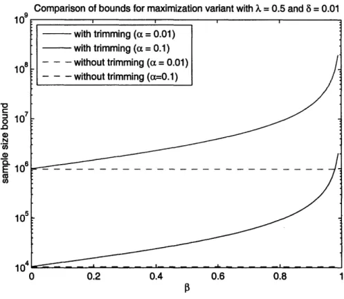
2-5 Comparison of bounds for the case of trimming and without trimming (trimming factor 0=0.05) as a function of the accuracy level a. .... . 57 2-6 Plot of the bounds for for the required number of samples in the
trim-ming case as a function of the trimtrim-ming factor p. ...
58
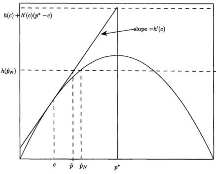
4-1 Illustration of h(c) for the case when 1RN < p**. ... 84 A-1 The sample average of the error of the SAA order quantity as a functionof the critical fractile A. ... 106 A-2 The accuracy level achieved by the sample average expected profit and
the sample average regret of the SAA order quantity as a function of the critical fractile A for various distributions. . ... 107
A-3 The accuracy level achieved by the sample average expected profit and the sample average regret of the SAA order quantity as a function of the mean p of the uniform distribution. .. ... 108 A-4 The accuracy level achieved by the sample average expected profit and
the sample average regret of the SAA order quantity as a function of the mean p of the normal distribution. . ... 109 A-5 The accuracy level achieved by the sample average expected profit and
the sample average regret of the SAA order quantity as a function of the standard deviation a of the normal distribution. ... 110 A-6 The accuracy level achieved by the sample average expected profit and
the sample average regret of the SAA order quantity as a function of the mean 1t of the exponential distribution. . ... 111 A-7 The accuracy level achieved by the sample average expected profit and
the sample average regret of the SAA order quantity as a function of the parameter k of the Pareto distribution. . ... . 112 A-8 The relative error of the regret achieved by the minimax regret
or-der quantity and the SAA oror-der quantity for the uniform and normal
distribution. ... ... .. 113
A-9 The relative error of the regret achieved by the minimax regret order quantity and the SAA order quantity for the exponential and Poisson
distribution. ... ... 114
A-10 The relative error of the regret achieved by the parameter-estimation order quantity and the SAA order quantity for the uniform and Pareto
distribution ... . ... 115
A-11 The relative error of the regret achieved by the parameter-estimation order quantity and the SAA order quantity for the exponential and
Poisson distribution. ... ... 116
A-12 The accuracy level achieved by the sample average expected profit and the sample average regret of the SAA order quantity as a function of
A-13 The accuracy level achieved by the sample average expected profit and the sample average regret of the SAA order quantity as a function of
the zero-price demand a... 118
A-14 The accuracy level achieved by the sample average expected profit and the sample average regret of the SAA order quantity as a function of the price-sensitivity parameter b. . ... . 119 A-15 The accuracy level achieved by the sample average expected profit and
the sample average regret of the SAA order quantity as a function of the mean p of the uniform distribution. . ... . . . 120 A-16 The accuracy level achieved by the sample average expected profit and
the sample average regret of the SAA order quantity as a function of the mean p of the exponential distribution. . ... 121 A-17 The accuracy level achieved by the sample average expected profit and
the sample average regret of the SAA order quantity as a function of the mean p of the normal distribution. . ... 122 A-18 The accuracy level achieved by the sample average expected profit and
the sample average regret of the SAA order quantity as a function of the standard deviation a of the normal distribution. . ... . 123 A-19 The accuracy level achieved by the sample average expected profit and
the sample average regret of the SAA order quantity as a function of the parameter k of the Pareto distribution. . ... 124
List of Tables
3.1 Theoretical and empirical confidence levels for various accuracy lev-els of the solution to the SAA counterpart of the profit-maximizing newsvendor with critical fractile A = 0.5 . ... 63 3.2 Theoretical and empirical confidence levels for various accuracy
lev-els of the solution to the SAA counterpart of the profit-maximizing newsvendor with critical fractile A = 0.9 . ... 64
Chapter 1
Introduction
In this thesis, we address several important variants of the classical newsvendor model, but under the assumption that the explicit demand distribution is not known. Rather, the only information available is a set of independent samples drawn from the true demand distribution. In particular, we consider three variants of the newsvendor model: the classical profit-maximization newsvendor model, the newsvendor model with risk preferences and the price-setting newsvendor model.
The classical profit-maximization model is a problem of matching supply and de-mand where the supply must be chosen before observing the dede-mand. Dede-mand is stochastic and the market parameters (i.e., price) are exogenous. In the classical model, the firm is risk-neutral and chooses an optimal ordering quantity that maxi-mizes its expected profit with respect to the full demand distribution. An extension of the classical model that incorporates risk preferences of a firm is the risk-averse newsvendor model which has been considered by Bertsimas and Thiele [5]. In this variant, the goal is to maximize the expected profit over a natural set of worst-case scenarios of the demand defined by the event that the demand is less than some spec-ified quantile. Another extension is the price-setting newsvendor model. This model apart from ordering decisions also incorporates pricing decisions. Under this model, the demand is stochastic and a function of price, and the firm decides simultaneously on the price and the supply level.
can be found either analytically or numerically via simulation methods. However, in real-life settings, the explicit demand distribution is not known. Typically, partial information on the demand is available from historical data or from simulations. Data-driven approaches can thus be used to solve the model under partial information. It is of interest to analyze the theoretical and empirical performance of these data-driven
approaches.
We discuss a nonparametric approach for solving the classical profit-maximization newsvendor model that makes use of observed samples of the demand without any assumptions on the true demand distribution. Levi, Roundy and Shmoys [24] consider a cost-minimization newsvendor variant and derive bounds on the number of samples required to ensure with high probability a good quality solution to the data-driven approach. We extend the results to the profit-maximization variant, and in fact significantly improve these bounds.
Bertsimas and Thiele [5] introduce a nonparametric data-driven approach based on one-sided trimming to solve the risk-averse newsvendor problem with partial in-formation on the demand. We provide a novel analysis regarding the number of samples required to ensure that the data-driven one-sided trimming method provides
a near-optimal solution with high probability.
For the price-setting newsvendor problem, Zhan and Shen [421 propose a simulation-based approach for a particular (i.e. linear-additive) form of the demand-price relation assuming that the parameters are known. The approach uses observed samples of the random component of the demand with only mild assumptions on its true distri-bution. By imposing additional assumptions on the distribution, we again obtain worst-case bounds on number of samples required for the simulation-based approach to provide a good quality solution with high probability.
Finally, through computational experiments, we verify the empirical performance of these data-driven approaches.
This thesis is structured as follows. In Chapter 2, we consider the classical newsvendor problem under imperfect information. We describe and analyze a non-parametric approach to the classical newsvendor problem. We also describe the
newsvendor problem with risk preferences and establish a connection between ac-curacy and the sample size of the one-sided trimming approach to the risk-averse newsvendor problem. In Chapter 3, we perform numerical experiments to evaluate the performance of the data-driven approach for the classical newsvendor problem under different concrete scenarios. We also compare its performance against other approaches that solve the newsvendor problem with partial information. In Chap-ter 4, we describe the price-setting newsvendor problem and analyze the simulation-based proposed by Zhan and Shen [42]. Finally, in Chapter 5, we conduct numerical experiments to evaluate the performance of the simulation-based approach to the price-setting newsvendor problem under different concrete scenarios.
Chapter 2
Data-Driven Approach to the
Newsvendor Problem with
Exogenous Price
In this chapter, we consider the classical profit-maximizing newsvendor problem with
exogenous price (i.e., price is not under the firm's control), but under the assumption
that the explicit demand distribution is not known. Instead, we assume that the only
information available is a set of independent samples drawn from the true demand
distribution. In this chapter, we discuss and analyze a data-driven approach based
on solving the Sample Average Approximation (SAA) counterpart. Specifically, we
provide a theoretical bound on the number of samples required to achieve a provably
near-optimal solution with high probability.
We consider a firm selling a product over a single sales period. A random demand
for the product occurs during the sales period. The firm needs to decide before the
sales period how many units of the commodity to produce. The actual demand occurs
during the sales period and is satisfied as much as possible with the units produced.
The firm incurs a cost proportional to the production quantity. The firm sells each
unit of product sold for an exogenously determined selling price. Any unmet demand
is assumed to be lost. The objective of the firm is to maximize its expected profit.
especially in revenue management. It can be applied to industries where the firm has no control over the price, but can influence its profit by deciding on a quantity of the product to order. Most industries selling perishable goods fit this criterion since the selling period is too short for the price to be adjusted. The model is also a building block for revenue management problems in the service industry such as airlines and hotels where there is allocation of limited resources to optimize profit.
Under full knowledge of the demand distribution, the classical newsvendor prob-lem has a well-defined solution that balances the expected cost of understocking and the expected cost of overstocking. Specifically, the optimal ordering quantity is a well-specified quantile of the demand distribution that can be computed if one knows the cumulative distribution function of the demand (Porteus [31]). In practice how-ever, the true demand distribution is usually not known. Instead, only partial and imperfect information is available on the demand in the form of demand parameters
(e.g., mean, variance, support) or historical demand data.
The newsvendor model and other inventory control and revenue management mod-els with imperfect demand information have been addressed by many researchers (e.g. Savage [34]; Scarf [36]; Gallego and Moon [15]; Bertsimas and Thiele [6]; Levi, Roundy and Shmoys [24]; Perakis and Roels [28]). When the demand distribution is unknown, one may use either a parametric approach or a nonparametric approach. A paramet-ric approach assumes that the true distribution belongs to a parametparamet-ric family of distributions, but the specific values of the parameters are unknown. On the other hand, a nonparametric approach requires no assumptions regarding the parametric form of the demand distribution.
A popular parametric approach pioneered by Scarf [35] to the newsvendor prob-lem uses a Bayesian procedure to update the belief regarding the uncertainty of the parameter based on observations that are collected over time. More recently, Liyan-age and Shanthikumar [25] introduced operational statistics as an approach which, unlike the Bayesian approach, does not assume any prior knowledge on the parameter values. Under this approach, optimization and estimation are done simultaneously.
informa-tion on the demand distribuinforma-tion in supply chain models. In this approach, instead of
fitting the data to a unique distribution, we allow a family of distributions to which
we assume the true demand distribution belongs. A traditional paradigm, called the
maximin approach consists of maximizing the worst-case profit over the set of
al-lowed distributions. Scarf [36] and Gallego and Moon [15] derive the maximin order
policy over family of distributions having the same mean and variance. The
diffi-culty with this approach is that it can lead to decisions under pessimistic scenarios
about the unknown demand. The robust minimax approach (Savage [34]; Perakis and
Roels [29]) is an alternative approach which somewhat relaxes this inherent
conserva-tiveness by introducing an "uncertainty budget" within which the worst-case scenario
is selected. The constraints are either ellipsoidal (see Ben-Tal and Nemirovski [2])
or polyhedral (Bertsimas and Sim [8]; Bertsimas and Thiele [6]). Other recent works
on the regret robust approach to other revenue management models include Ball and
Queyranne [1], Eren and Maglaras [13] and Perakis and Roels [28]. This approach
minimizes the maximum opportunity cost for not making the optimal decision. The
robust approach works well if the only information available are market demand
para-meters such as the mean or variance. Note that these approaches no longer consider
the original objective of maximizing the expected profit. Moreover, the resulting
solution may be very conservative.
Several nonparametric approaches have been applied to inventory models and the
newsvendor problem with partial demand information. The concave adaptive value
estimation (CAVE) approach (e.g. Godfrey and Powell [17]) successively
approxi-mates the objective cost function with a sequence of piecewise linear functions. The
infinitesimal perturbation approach (IPA) is a sampling based stochastic gradient
es-timation technique that has been used to solve stochastic supply chain models (see
Glasserman and Ho [16]). The bootstrap method (Bookbinder and Lordahl [9]) is
a nonparametric approach that estimates the newsvendor quantile of the demand
distribution. More recently, Huh and Rusmevichientong [20],[19] develop an
adap-tive algorithm for capacity allocation problems and inventory planning problems with
censored demand data.
Another nonparametric approach that utilizes realizations of the demand is the data-driven approach. This approach has the advantage that realizations of the de-mand are easily obtained from dede-mand data of past periods. From a practical stand-point, the data-driven approach is a simple and natural means to provide an accurate estimate of the optimal order quantity. One such data-driven approach that solves stochastic optimization problems by using only samples of the random variable is the Sample Average Approximation (SAA) approach. In the SAA approach the origi-nal objective function, which is the expectation of some random variable, is replaced with the average of the random samples. The SAA approach has been considered for two-stage stochastic optimization models by Kleywegt, Shapiro and Homem-De-Mello [23]. They show that the optimal value of the SAA approach converges to the optimal value of the original problem with probability 1 as the sample size goes to infinity. They also derive bounds on the sample size that ensures with a confidence probability that the difference between the objective value of the SAA solution and the optimal objective value is a certain value. The bounds they derive however, de-pend on the variance and other properties of the objective function which might be
difficult to know if the demand distribution is not known.
Levi, Roundy and Shmoys [24] apply the SAA approach to the cost-minimizing newsvendor problem. Under this variant of the newsvendor model, the firm chooses an order quantity to minimize its expected cost under the presence of an understocking cost b and an overstocking cost h. In this model, it is optimal to order the bb+h quantile of the demand. Levi, Roundy and Shmoys [24] derive a bound on the sample size that ensures a good quality solution to the SAA approach with high probability. In particular, they show that if the sample size is greater than log
(),
wheremin(b,h) b+h I then the solution of the SAA counterpart is at most 1 + a times the
optimal solution under full knowledge of the distribution with probability at least 1 - 6. In contrast to [23], the bound they derive is easy to compute and is free of any assumptions on the demand distribution.
However, applying the bound in [24] for the SAA counterpart of the profit-maximizing variant is not straightforward. In fact, it is usually the case that
approx-imation results for minimization problems do not directly translate to approxapprox-imation results for the equivalent maximization problem. In this chapter, we introduce a new notion of regret, which we define as the expected cost of the uncertainty in the demand. In particular, it is the difference in the expected profit under the scenario where the firm knows the demand beforehand and the profit under the scenario where the demand is uncertain. By introducing this concept, we managed to leverage the bound in [24] and apply it to the profit-maximization newsvendor problem. Moreover, we managed to improve on the bound in [24] and obtain a significantly stronger the-oretical bound that is inversely proportional to w instead of w2.For example, in the cost-minimization newsvendor model, if the service level - is high, as is typically the case in practice, then we significantly improve (in terms of order of magnitude) the bound on the required sample size that ensures that the SAA approach provides an accurate solution.
Finally, we extend the data-driven approach to newsvendor models that incor-porate risk. Bertsimas and Thiele [5] consider a variant of the classical newsvendor problem that incorporates risk preferences of the firm. In the traditional model, the optimal order quantity is determined by maximizing the expected profit with respect to the whole demand distribution. In contrast, they assume that the firm maximizes the expected profit over a natural set of worst-case scenarios of the demand defined by the event that the demand is less than some specified risk parameter. Bertsimas and Thiele [5] propose a data-driven approach to approximate the solution of the risk-averse newsvendor problem. By considering their approach as a variant of the SAA counterpart of the risk-neutral problem with adjusted parameters, we provide a novel analysis regarding the number of samples required to guarantee with a specified confidence level that the regret of the solution to their approach is a near-optimal approximation of the regret under full knowledge of the distribution.
The remainder of this chapter is structured as follows. In Section 2.1, we consider the problem under full knowledge of the demand distribution and review optimality conditions for the solution to this problem. In Section 2.2, we assume imperfect infor-mation about the demand in the form of samples from the true demand distribution.
We introduce the SAA counterpart of the problem that provides us an approximate solution to the newsvendor problem. In Section 2.3, we will address the question of finding a sample size that ensures that the SAA counterpart is a "good" approxima-tion of the original newsvendor problem. Finally, in Secapproxima-tion 2.4, we find a bound on the sample size for the data-driven approach by Bertsimas and Thiele [5] that ensures an accurate solution to the problem with risk preferences.
2.1
The Profit-Maximizing Newsvendor Model
In this section, we consider the classical maximization newsvendor problem. The classical newsvendor model deals with determining an optimal order level to maxi-mize profit under uncertain demand. Under this model, it is assumed that the ex-plicit demand distribution is known. We provide a mathematical formulation of the profit-maximizing newsvendor problem with exogenous price. The optimal solution is characterized by a balance between the expected cost of understocking and expected cost of overstocking. Porteus [31] and Khouja [22] provide excellent summaries of this problem.
2.1.1
Problem Formulation
First we define the following notation, which will be useful throughout the chapter: c unit cost,
p unit selling price,
q order or production quantity, D random demand with mean /p, F(.) cumulative distribution of demand.
We define the monotonically non-increasing, left-continuous function
F(d) = Pr(D > d), (2.1)
A random demand D for a single commodity occurs in a single period. At the beginning of the period, before the demand is observed, the firm decides to order q units of the commodity to satisfy the random demand D. The cost to order a unit of the commodity is c. During the selling period, the actual demand d (the realization of D) is observed. The firm sells the minimum of the demand and the number of units ordered, at a unit selling price p. The profit of the firm is given by
ir(d,
q) = p min(d, q) - cq.Since the actual demand is not known when ordering decisions are made, a sensible objective for the firm is to maximize the expected profit. Thus, the problem is equivalent to solving
max g(q), (2.2)
q>O
where
g(q) = E[ir(D, q)] = p E[min(D, q)] - cq
is the expected profit of the firm for a given order quantity, q. Unless stated otherwise, the expected value is taken with respect to the true demand distribution. We refer to problem (2.2) as the maximization variant of the newsvendor problem.
A standard assumption in the classical newsvendor problem is that the unit price exceeds the unit cost (i.e., p > c). Otherwise, there is no incentive for the firm to order any units of the commodity. Note that, without loss of generality, the salvage cost for each unit of excess inventory is assumed to be equal to zero.
We can think of the cost of uncertainty in the newsvendor model as the differ-ence between the expected profits under the scenario where the demand is known beforehand and when the demand is uncertain. If the expectation of the demand infi-nite, then any ordering cost will incur negative uncertainty cost. Thus, the following assumption is needed for the newsvendor problem to be well defined.
2.1.2
Optimal Solution
In this subsection, we characterize the optimal order quantity of the maximization variant of the newsvendor problem (2.2). Recall that a profit-maximizing firm seeks to find an order quantity that maximizes its expected profit function. That is, the firm wishes to maximize g(q) with respect to q. Note that g(q) is a concave function. Thus, in order to find the order quantity that maximizes g(q), we can utilize standard results in convex optimization. The following properties of a concave function are discussed thoroughly in Bertsekas [7].
Definition 2.1.1 (Bertsekas [7, p. 731]) Let f : R" --+ R be a concave function. A vector v E Rn is a subgradient of f at a point x0o if for any x E Rn, f(x) 5 f(xo) + vT(x - xo). We denote the set of all subgradients of
f
at x0o as the subdifferential,Of(xo).
Theorem 2.1.1 (Bertsekas [7, pp. 731-732]) Let f : 9R -+ - be a concave function. Then x0o is a global maximizer of f if and only if 0 E
Of(xo).
If f : R -- R is a concave function, one may show that the subdifferential at x0o is a nonempty closed interval [fr(xo), fl(xo)], where f'(xo) and fr(xo) are the left-sided and right-sided derivatives at xo.
Since g(q) is a concave function, then we can use the optimality condition for a concave function stated in Theorem 2.1.1. Note that the left-sided and right-sided derivatives of g(q) are given by
g'(q) = p(1 - Pr(D<q)) - c,
gT(q) = p (1 -F(q)) - c.
If the cumulative distribution function of D is continuous, note that g9(q) - gr(q) =
g'(q).
For simplicity, let us define
c
A = 1 - -. (2.3)
which is referred to in the literature (see Porteus [31]) as the critical fractile. The critical fractile A balances the cost of understocking (each unit of lost sale is worth (p - c)) and the cost of overstocking (the cost of each unit of unused supply is c).
Define
q*= inf {q F(q) > A}, (2.4)
where A is given by (2.3).
Since gl(q*) > 0 and gr(q*) < 0, then we know that 0 E 9g(q*). By Theorem 2.1.1, q* is the production quantity that optimizes g(q). Thus, the optimal policy is to order up to the A quantile of demand.
If the cumulative distribution function of the demand is known, then we can ex-plicitly solve for the optimal order quantity, q*. However, in most real-life scenarios, the true demand distribution is not available. Usually, the information that is avail-able comes from historical demand data. In the following section, we will introduce a data-driven approach based on solving the Sample Average Approximation (SAA) counterpart.
2.2
Sample Average Approximation
One common approach for solving stochastic optimization problems is to solve the Sample Average Approximation (SAA) counterpart. In the original problem, the objective function is the expectation of some random function taken with respect to the true underlying probability distribution. In the SAA counterpart, the objective function is the average value over finitely many independent samples that are drawn from the probability distribution. Shapiro [38] provides an excellent overview of the SAA approach to solving stochastic optimization problems.
Under full knowledge of the demand distribution, the optimal ordering quantity q* is the A quantile of the demand distribution. Suppose the demand distribution is unknown and the only information available is a set of independent samples of the demand. We can estimate the expected profit by a function that depends on realizations of the demand. Specifically, for a set of N independent samples of the
demand D, denoted by dl,..., d". We approximate the original objective function by
N
maxg(q) = p min (q,dk) - cq. (2.5)
k=l
The SAA counterpart can be thought of as a modified newsvendor problem defined with respect to the induced empirical distribution where each of the N samples of the demand occurs with the same probability 1
Let QN denote the optimal solution to the SAA counterpart with N samples. Note that
QN
is a random variable that is dependent on the specific N samples of D. Since the SAA counterpart is a modified newsvendor problem defined on the empirical distribution, the A sample quantileN= inf
{qlFN(q) >
A (2.6)is a realization of QN, where -FN(q) is the cumulative distribution function of the empirical distribution. The empirical distribution has the following distribution func-tions: N
FN(q)
Z
1(dk
<
q),
(2.7)
k=1 N FN(q) = - l(dk > q). (2.8) k=1where 1(.) is the respective indicator function which is equal to 1 when the argument is true.
2.3
Relative Error of the Regret of the Optimal
Solution to the SAA Counterpart
The SAA approach relies on samples of the demand to approximate the expected profit function. A natural question to ask is how many samples are required to
ensure with high probability a good quality solution of the SAA counterpart? Levi, Roundy and Shmoys [24] address this question for the cost-minimizing newsvendor problem. We define the cost-minimization variant as follows. Consider the case when a firm wishes to choose an order quantity that minimizes its expected cost. Let q be the order quantity. If the number of units ordered exceeds the actual demand, then a per-unit holding cost, h, is incurred for each unit of excess inventory. On the other hand, if the actual demand exceeds the number of units ordered, then a per-unit lost-sales penalty, b, is incurred for each unsatisfied demand. The goal in this minimization variant is to choose an order quantity that minimizes the expected cost, given these costs. Thus, the problem is to solve
min C(q) = E [h(q - D)+ + b(D - q)+] (2.9) q>0
where x+ = max(x, 0). We refer to problem (2.9) as the minimization variant of the newsvendor problem. Suppose qA is the optimal order quantity of the cost-minimizing newsvendor problem. Then it can easily be shown that q;, is the -L quantile of the
demand distribution [24].
Levi, Roundy and Shmoys [24] apply the SAA approach to solve the cost-minimizing newsvendor problem. The optimal order quantity of the SAA counterpart
Q1
is theb quantile of the implied empirical demand distribution. They establish how the
accuracy of the SAA counterpart relates to the sample size. In particular, they obtain a bound on the number of samples N = N(b, h, a, 6) required to guarantee that, with probability of at least 1 - 6, the optimal solution to the SAA counterpart defined on N samples has an expected cost C(Q() of at most (1 + a)C(q;). The following theorem holds.
Theorem 2.3.1 (Levi et al. [24, Theorem 2.2]) Suppose Assumption 2.1.1 holds. Consider the cost-minimizing newsvendor problem specified by a per-unit holding cost h > 0 and a per-unit backlogging penalty b > 0. Let 0 < a < 1 be a specified accuracy level and 1 - 6 (for 0 < 6 < 1) be a specified confidence level. Suppose that N > -2a 2W log 2
(
6', ), where w = min(b,h) b+h Suppose the SAA counterpart is solvedwith respect to N i.i.d. samples of D. Let
Q7
be the optimal solution to the SAA counterpart. Then, with probability of at least 1- 6, the expected cost ofQ7'
is at most 1 + a times the expected cost of an optimal solution q* to the newsvendor problem. In other words, C(Qm) < (1 + a)C(q ) with probability of at least 1 - 6.To prove Theorem 2.3.1, Levi, Roundy and Shmoys [24] introduced the follow-ing property that relates to the accuracy of a solution as an approximation to the subgradient conditions.
Definition 2.3.1 Let •q be some realization of
Qm
and let a' > 0. We will say that qM is a'-accurate if F(@) ~ -b+h
- a' and F(q•) N-> - a'.In what follows we discuss the steps behind the proof of Theorem 2.3.1 in [24]. In the first step it is shown that if •q is
a'-accurate,
witha'
= min(b,h) then itsexpected cost is at most (1 + a)C(q*). Next, it is shown what is the number of samples N = N(a', 6) required to guarantee that the 6 quantile of the N samples of the random demand is a'-accurate with a confidence probability 1- 6. Theorem 2.3.1 follows by combining these two steps. The following two results outline these steps rigorously.
Corollary. 2.3.2 (Levi, Roundy and Shmoys [24, Corollary 2.1]) For a given accu-racy level a E (0, 1], if q M is a'-accurate for a' = mi(b,h) then the cost of 4m is at most (1 + a) times the optimal cost, i.e., C(4m) < (1 + a)C(qm).
Lemma 2.3.3 (Levi, Roundy and Shmoys [24, Lemma 2.2]) For each a' > 0 and 1, if
the number of samples is N
>
N(a', 6) =
1 log(2),
then Qý,
the b-hquantile of the sample, is a'-accurate with probability of at least 1 - 6.
It is relatively straightforward to see that the definition 2.3.1 of a'-accuracy is related to the deviation between the CDF of the empirical and the true demand distribution, as well as the deviation between the function F of the empirical and the true demand distribution. In particular, the proof of Lemma 2.3.3 is based on the well-known Hoeffding's inequality that is used to bound these deviations.
Theorem 2.3.4 (Hoeffding's Inequality [18]). Let Xl,...,XN be i.i.d. random
variables such that X1 E [, 13] for some a < P. Then, for each e > 0, we have
Pr
(_
k
Xi
-
E[X
1
]
>
<
e-2C•N/(p-a)2
It must be noted that (1 + a)-accurate approximations of the objective function of a minimization problem do not necessarily translate to (1 + a)-accurate approx-imations of the objective function of a maximization problem. In fact, it is usually the case that approximation results for minimization problems cannot be leveraged to the equivalent maximization problems. Thus, applying Theorem 2.3.1 to the profit-maximization newsvendor problem is highly nontrivial.
It is natural to think of an approximation to the newsvendor problem being "good" if the relative error of its expected profit is small. With this criterion however, a possible complication is that the expected profit of the optimal order quantity is not guaranteed to be well above zero.
To circumvent this problem, we introduce the notion of regret. We define the regret as an objective function of a minimization problem equivalent to the profit-maximization newsvendor problem. If we can show that the approximation evaluated at the regret function has a small relative error, then we can say that it is a "good" approximation.
If the firm knows beforehand that it will face a demand of d, then it will order exactly d units to cover the demand. Ordering any more or less units will give the firm marginal costs. Therefore, under the scenario where the demand is known prior to ordering, the firm makes an expected profit of (p - c)pI. The firm cannot achieve a better profit than this if the demand it faces is unknown. We can think of the difference between (p - c)IL and the expected profit if the demand is unknown as the cost of the demand uncertainty. Therefore, the profit-maximizing strategy of the firm also minimizes the cost of uncertainty of the demand.
We define the regret to be the difference between the expected profit when the demand is known and the expected profit under uncertain demand. That is, the regret function is
Note that the regret function is minimized by the optimal solution to the newsvendor problem, q*.
In what follows, we reduce the profit-maximizing newsvendor model into the cost-minimization variant of the newsvendor problem using some suitable transformation. By doing so, we can apply the results derived in Levi, Roundy and Shmoys [24] for the SAA counterpart to the profit-maximizing newsvendor.
Consider the profit-maximizing newsvendor problem (2.2). After rearranging terms, we can rewrite
pE [min(D, q)] = pE [D + min(q - D, 0)] = pE [D - (D -q)+]
= pp-pE [(D-q)+]
where E[D] = p, and
-cq-cE[(D-q)+] +cy = -cE[q+max(D-q,O)-D]
= - cE [(q - D)+].
Thus, the expected profit of the newsvendor problem can be rewritten as
g(q) = p E[min(D,q)] - c q
= p (M -E[(D-q)+]) -cE[(q-D)*] +cE[(D-q)*] -cm = (p- c)p- E [c(q- D)+ + (p- c)(D- q)+].
This implies that the regret p(q) can be expressed as
p(q) = (p - c)m - g(q) = E [c(q - D)+ + (p - c)(D - q)+] . (2.11)
Note that equation (2.11) implies that, for every unit of quantity above the actual demand, a cost of c is incurred. On the other hand, for every unit of demand above the order quantity, a cost of p - c is incurred. Thus, the regret represents the cost of
a mismatch between the demand and supply (see Cachon and Terwiesch [10]). If we introduce the transformation
C(q) = p(q), (2.12)
h = c, (2.13)
b = p-c, (2.14)
then we find that minimizing the regret p(q) of the profit-maximizing newsven-dor is equivalent to the cost-minimization variant considered by Levi, Roundy and Shmoys [24]. Also note that under this transformation, the b quantile is equal to
the A quantile. Thus, it follows that 4N =
@q
and q* = q*.Therefore, we have the following version of Corollary 2.3.2.
Corollary. 2.3.5 For a given accuracy level a E (0, 1], if qN is a'-accurate for a' = yw where w = min(A, 1- A), then the regret of N is at most (1 +a) times the optimal regret, i.e., p(qN) • (1 + a)p(q*).
Next we shall show that the bound in Theorem 2.3.1 can be significantly improved to depend only on 3 instead of 1. We state this result:
Theorem 2.3.6 Suppose Assumption 2.1.1 holds. Consider the profit-maximizing newsvendor problem specified by a unit selling price p > 0 and a unit production cost c > 0 (where p > c). Let 0 < a < 1 be a specified accuracy level and 1 - 6 (for 0 < 6 < 1) be a specified confidence level. Suppose that N > N(w, a, 6)
- (9(1 - w) + 4a) log
()
where w = min(E, 1- !). Suppose the SAA counterpart is solved with respect to N i.i.d. samples of D. Let QN be the optimal solution to the SAA counterpart. Then, with probability of at least 1 - 6, the regret of QN is at most 1 + a times the regret of an optimal solution q* to the newsvendor problem. In other words, p(QN) _ (1 + a)p(q*) with probability of at least 1 - 6.Observe that the bound in Theorem 2.3.6 is inversely proportional to w. We contrast this to the bound in Levi, Roundy and Shmoys [24] which is inversely pro-portional to w2. If w is small, then the ratio between the cost of being understocked
and the cost of being overstocked is either very big or very small. In most industries, w is typically small. Therefore, this result significantly reduces sample size (i.e. in order of magnitude) that is required to ensure that the SAA counterpart provides an accurate approximation of the optimal regret with a certain confidence level.
The idea behind the proof of Theorem 2.3.6 is that we replace and strengthen Lemma 2.3.8. As mentioned previously, the proof of Lemma 2.3.3 makes use of Ho-effding's inequality. HoHo-effding's inequality provides an upper bound on the probability that a sum of random variables deviates from its mean using only information about the support of the random variables. We can think of Hoeffding's inequality providing this bound by assuming the worst possible variance with only the knowledge of the range. However, if additional variance information is available, then a tighter bound can be found by using Bernstein's inequality. Below we state Bernstein's inequality:
Theorem 2.3.7 (Bernstein's Inequality [4]). Let X1,... ,XN be i.i.d. random
vari-ables satisfying Pr(Xi - E[X1]
<
d) = 1. Let C2 = E[Xj2] - E[X1]2. Then for anyS> 0,
1
-NE2
Pr X-E[X] >E < exp 2d.
P Ni= 1 - 3
Note that for a fixed q, we can define X' = X (q) = 1(di < q). Suppose we have N samples of the demand. Therefore, FN(q) = j , Xk. Note that, E[X1 ] = F(q), a2 = F(q)(1 - F(q)), and X1 - E[X1] < 1. Thus, taking d = 1 and applying
Bernstein's inequality, it follows that for each q
Pr (FN(q) - F(q)> E) < exp
(
±
.3 (2.15)2F(q)(1 - F(q))
+2E
Similarly, we can define Z' = ZP(q) = 1(di > q) for a fixed q. For N samples of the demand, we have
FN(q)
=k
Zk. Note that E[Z1]
= F(q), a2 = F(q)( - F and Z' - E[Z1 ] < 1. Taking d = 1, we can apply Bernstein's inequality, to obtainPr
FN(q)
- F(q) > E < exp (q)(1 q)) (2.16)2F(q)(1 - F(q)) + 23
By using Bernstein's inequality, we obtain a stronger version of Lemma 2.3.8:
Lemma 2.3.8 For each a' > 0 and 0 < 6 < 1, if the number of samples is N > N(w, a', 6) = (w(1 - w) +
) log
(),
where w = min (1 - A, A), then QN the Aquantile of the sample is a'-accurate with probability of at least 1 - 6.
Proof. Note that each given sample of size N of the demand, qN is the A quantile of the empirical distribution. Define the event
B = [F(N) < A--a].
Also define the quantile
qi = inf {qF(q) > A-a'}
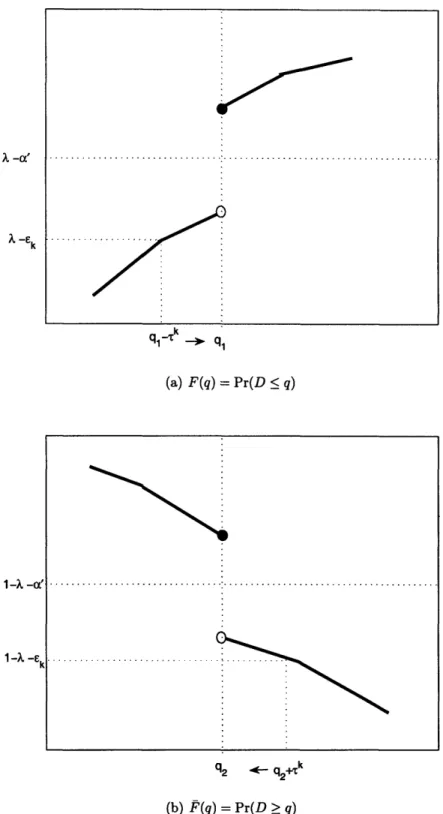
which is illustrated in Figure 2-1(a).
Since F(.) is nondecreasing, then B = [qN < qi]. Consider a monotonically decreasing, nonnegative sequence {Tk}, where Tk I 0. Define the events
Bk= [FN (ql - rk) A] = [N • 1 -_7k]
Note that since FN(ql - Tk) N(ql - rk+1), then it follows that Bk C Bk+1.N< Thus, if B is the limiting event of the sequence of events {Bk}, then Bk T B. Thus, Pr(Bk) T Pr(B). Note also that B C B. This implies that Pr(B) •< Pr(B).
From the definition of ql, note that for every k, there exists Ek > a' such that F(qx - rk) = A - ek < A - a'. Note that
k -a' it-E ql -Tk --> ql (a) F(q)= Pr(D < q) 1
-
-a'. 1- . -E... ... q2 4q2- k (b) F(q) = Pr(D > q)Figure 2-1: Illustration of a cumulative distribution function, F, and distribution function, F, and the quantiles ql and q2.
Thus, we have
Pr(Bk) = Pr(FN(q- Tk)>A)
= Pr(FN(q1 - Tk) - F(qi - Tk) > Ek)
< exp - NE k ))2/2
(F(qi
-
Tk)(1
- F(q, -
k))
+3
where the last inequality follows from (2.15) by Bernstein's inequality. From (2.17), it follows that
Pr(Bk) <
exp
(( = exp ( -NEck2/2-
a')(1
-
A
+
Ek)+
3 1(A--NEk/2-
a')(1
- A)
+
A
-a' +
13Since Ek > a', then
Pr(Bk) < exp - (AA = exp (1A(
Also, since w = min(A, 1 - A), then
Pr f R 1 < ovn -Na'/2
- a')(1 - A) + A
-
a' +
-
A)
-
ý +
2A
- a' ) -w)+
-2w-(
-Na'/2 <exp
1 (1 W 4 " 7W - 3) Thus, by choosing N - w(1 - w) +1) log()we then have Pr(Bk) for all k, which implies that Pr() < " Pr(B) < "
Therefore, .
J
Now define the event
L = [F(N)< < - A -'.
Also define the quantile
q2 = sup
{q
(q) 1 -A-
a'}.
which is illustrated in Figure 2-1(b).
Since F(.) is non-increasing, then L = [4N > q
2]. Define the events
Lk
[
FN(q2
+
Tk)>
1--]
[N> q
2+
Tk]
Note that since FN(q
2+
Tk)<
FN(q2 +
Tk+l),then it follows that Lk
C
Lk+1l
Thus, if L is the limiting event of the sequence of events {Lk}, then Lk
I
L. Thus,
Pr(Lk)
I
Pr(L). Note also that L C L. This implies that Pr(L) < Pr(L).
From the definition of
q2,
note that for every k, there exists sk > a' such that
F(q
2 Tk)1
-
A
-
Ek < 1
-
A
-
a'. Note that
F(q2
+
Tk1)(q2
+ Tk)) <(1 -
-
)(A
+k).
(2.18)
Thus, we have
Pr(Lk)
= Pr(FN(q2 +rTk )l _= Pr(FN(q
2+ k) -
(q
2 + Tk) _> k)Sexp (
- Ne
2/2
F(q2
+
Tk)(1
- F(q2
+
7k)) +
1
From (2.18), it follows that
Pr(Lk) < exp
-Nek2/2-exp(
-Nek/2Thus, based on similar arguments we can conclude that choosing
N >
4
I1w(1
-
w) + )log (
implies that Pr(Lk) < _ for all k. It follows that Pr(L) • Pr(L) < d.
Note that [QN is not a'-accurate] = B U L. Thus, Pr(QN is not a'-accurate) < Pr(B) + Pr(L) < 6. Thus, for
N N(w, a, 6) = w(1 - w) + - log ,
we have Pr(QN is a'-accurate) > 1 - 6.
I
We can now proceed to prove Theorem 2.3.6, which makes use of Bernstein's inequality.
Proof of Theorem 2.3.6. Suppose a' = '. Then, from Lemma 2.3.8, for N > --; w(l-w) + log
S (1 - w) + -4 log(2
aw
a
3
1jg
6
= (9(1 - w)
+ 4a) log
-a2w
it follows that QN is a'-accurate with probability of at least 1 - 6. Since if qN is a'-accurate, it follows by Corollary 2.3.5 that p(qN) < (1 + a)p(q*). This concludes the proof of the theorem. I
newsvendor and the objective function of the cost-minimizing newsvendor are equiv-alent we can extend Theorem 2.3.6 to the cost-minimization variant.
Theorem 2.3.9 Suppose Assumption 2.1.1 holds. Consider the cost-minimizing newsven-dor problem specified by a per-unit holding cost h > 0 and a per-unit backlogging penalty b > 0. Let 0 < a < 1 be a specified accuracy level and 1-6 (for 0 < 6 < 1) be a specified confidence level. Suppose that N > N(w, a, 6) - (9(1 - w) + 4a) log(
),
where w = min(h) Suppose the SAA counterpart is solved with respect to N i.i.d. samples of D. LetQ7'
be the optimal solution to the SAA counterpart. Then, with probability of at least 1 - 6, the expected cost ofQ•
is at most 1 + a times the ex-pected cost of an optimal solution q* to the newsvendor problem. In other words,C(Qg) < (1 + a)C(q*) with probability of at least 1 - 6.
We observe that the Hoeffding sample size bound is of the order of magnitude proportional to 1 log
(
).
On the the other hand, the Bernstein sample size bound is of the order of magnitude proportional to -I log(
).
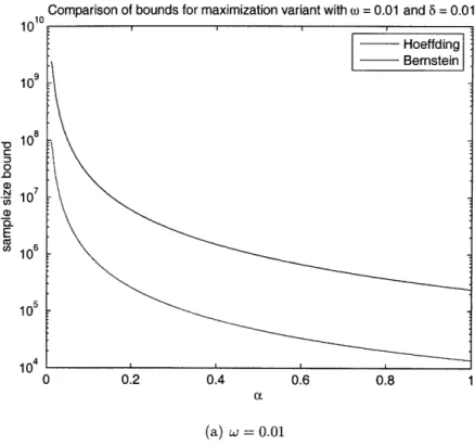
Therefore, for small values of w, we expect that the Bernstein sample size bound is significantly smaller than the Hoeffding bound. Note that if w is small, the optimal order quantity belongs to extreme quantiles of the demand distribution.Figures 2-2 and 2-3 illustrate the difference in the bounds provided by Bernstein and Hoeffding for various levels of w. Notice that if w is close to zero, then there is a drastic improvement on the sample size required by the Bernstein bound. On the other hand, if w is close to 1, then the difference between the two bounds is negligible. Therefore, if w is significantly small, then we can expect a significant improvement in the order of magnitude of the sample size required by the Bernstein bound. On the other hand, for the ranges where the Hoeffding bound is better, the improvement is small.
In the following lemma, we establish conditions on the parameters that would guarantee that Bernstein's inequality provides a tighter bound on the sample size. For each accuracy level, the range of w values for which the Bernstein or Hoeffding
Comparison of bounds for maximization variant with w = 0.01 and 8 = 0.01
0 0.2 0.4 0.6 0.8 1
(a) w = 0.01
Comparison of bounds for maximization variant with 0) = 0.05 and 8 = 0.01
0 0.2 0.4 0.6 0.8 1
(b) w = 0.05
Figure 2-2: Comparison of bounds implied by Hoeffding, and Bernstein for the max-imization variant of the newsvendor problem as a function of the accuracy rate, for w = 0.01, 0.05.
Comparison of bounds for maximization variant with w = 0.2 and 8 = 0.01
0.2 0.4 0.6 0.8 1
(a) w = 0.2
Comparison of bounds for maximization variant with o = 0.4 and 8 = 0.01
j A7
0.2 0.4 0.6 0.8 1
(b) w = 0.4
Figure 2-3: Comparison imization variant of the w = 0.2, 0.4.
of bounds implied by Hoeffding, and Bernstein for the max-newsvendor problem as a function of the accuracy rate, for
106 0 10 10 Q) N (u E 104 10 3 0 10U
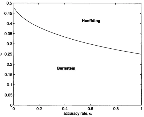
bound gives tighter bounds are plotted in Figure 2-4.
Lemma 2.3.10 For a specified accuracy level a > 0 and a specified confidence level 1 - 6 (for 0 < 6 < 1), the Bernstein bound in Theorem 2.3.9 is smaller than the
Hoeffding bound in Theorem 2.3.1 if and only if w
<
L (9 + 4a - 4a(4a + 18)).
Proof. From Theorems 2.3.1 and 2.3.9, it follows that Bernstein's inequality gives a better bound if and only if
9
9w2 - (9 + 4a)w + -> 0. (2.19)
4-For a fixed a, the left-hand side of (2.19) is a second degree polynomial of w. The discriminant of (2.19) is given by
A
=
(9 + 4a)2 - 92 = 4a (4a + 18), (2.20)which is always nonnegative. Therefore, if we define
Wmin = 9 + 4a - ,
18 9+4•- ,
wmax = 9
+
4a+
,
then the bound provided by Hoeffding's inequality in Theorem 2.3.1 is better than
Bernstein in Theorem 2.3.9 only in the range of w E [wmin, Wmax]. Note however thatA > 16a
2. Thus,
Wmax =
(9 + 4+x/
V)
1 1
>
-(8a
+ 9) > -.18 -2
Since w = min
m,
1
-
, we know that w <•
.
Thus, a necessary and sufficient
3
0 0.2 0.4 0.6 0.8 1
accuracy rate, a
Figure 2-4: Plot of regions of w = min (1 - A, A) for which the Hoeffding or the Bernstein bound is tighter, for various accuracy rates, a. The y-axis is in logarithmic scale.
2.4
The Newsvendor Model with Risk Preferences
The assumption of the newsvendor problem discussed in Section 2.1 is that the firm is risk-neutral. However, under an experimental setting, it has been shown by Schweitzer and Cachon [37] that ordering choices systematically deviate from those that maxi-mize expected profit. The firm will often accept a smaller expected profit if it also yields a smaller risk of returns. Bertsimas and Thiele [5] model this risk-preference by introducing a single scalar risk parameter that allows the firm to adjust the trade-off between risk and return. Under a traditional newsvendor model, a risk-neutral firm chooses an ordering quantity that maximizes its expected profit with respect to all of the demand scenarios. In contrast, under the model they propose in [5], a risk-averse firm will choose to protect itself only against a specified set of worst-case scenarios of the demand. In particular, it will choose an ordering quantity that maximizes the expected profit conditioning on the demand being less than some specified risk para-meter. They call this one-sided trimming of the demand. Moreover, Bertsimas and Thiele [5] propose a data-driven approach based on one-sided trimming to approxi-mate the optimal order quantity under the newsvendor setting with risk preferences. In this section, we provide a novel analysis regarding the quality of the solution of their data-driven approach. The analysis is based on a variant of the SAA approach under the risk-neutral setting, but with appropriately adjusted parameters.
Suppose 3 is a risk parameter, where
/
E (0, 1). Let qp be the 1 - /3 quantile of the random demand D. That is,qP = inf{qlFD(q) > 1 - 0}.
Without loss of generality, we can assume that FD(qp) = 1 - 3. This is because if there is a probability mass on qp and FD(qp) > 1 - P, then we can decrease
/3
until this property is satisfied without increasing the risk.A risk-averse firm will choose a conservative ordering policy that maximizes its expected profit conditional on the event that D < qp. Define the random variable D = [DID < qp]. To avoid confusion, all functions and expectations will be subscripted