HAL Id: tel-00732658
https://tel.archives-ouvertes.fr/tel-00732658
Submitted on 16 Sep 2012
HAL is a multi-disciplinary open access
archive for the deposit and dissemination of
sci-entific research documents, whether they are
pub-lished or not. The documents may come from
teaching and research institutions in France or
abroad, or from public or private research centers.
L’archive ouverte pluridisciplinaire HAL, est
destinée au dépôt et à la diffusion de documents
scientifiques de niveau recherche, publiés ou non,
émanant des établissements d’enseignement et de
recherche français ou étrangers, des laboratoires
publics ou privés.
the human brain at ultra high field : specific absorption
rate control & flip-angle homogenization
Martijn Anton Hendrik Cloos
To cite this version:
Martijn Anton Hendrik Cloos. Parallel transmission for magnetic resonance imaging of the human
brain at ultra high field : specific absorption rate control & flip-angle homogenization. Other
[cond-mat.other]. Université Paris Sud - Paris XI, 2012. English. �NNT : 2012PA112066�. �tel-00732658�
ÉCOLE DOCTORALE : STITS
Laboratoire de : NeuroSpin
DISCIPLINE : Physique
THÈSE DE DOCTORAT
soutenue le 17/04/2012
par
Martijn Anton Hendrik CLOOS
Parallel Transmission for Magnetic
Resonance Imaging of the Human Brain at
Ultra High Field
Specific Absorption Rate Control & Flip-Angle Homogenization
Directeur de thèse : Denis Le Bihan Dr. MD. (Directeur de NeuroSpin)
Composition du jury :
Président du jury : Luc Darrasse Dr. (Directeur de l’IR4M au CNRS)
Rapporteurs: Cornelis van den Berg Dr. Ir. (Directeur de recherche à l’Hôpital de l’Université d’Utrecht) Maxim Zaitsev Dr. (Directeur de recherche à l’Hôpital de l’Université de Freiburg) Examinateur : Hans-Peter Fautz Dr. (Ingénieur chercheur à Siemens Healthcare)
Encadrant : Alexis Amadon Dr. (Ingénieur chercheur à NeuroSpin)
This thesis is submitted in partial fulfillment of the requirements for the Degree of Doctor of Philosophy at University Paris-Sud XI. The results presented herein are based on the author’s scientific endeavors performed between February 2009 and January 2012 at NeuroSpin. In the framework of the Franco-German Iseult-INUMAC project, and in anticipation of the whole body 11.7-Tesla magnetic resonance imaging setup, this work focuses on the development of parallel-transmission strategies to maximize the performance of current and future ultra-high field systems. Apart from aspiring to the realization of the above-mentioned goals, the author hopes this writing will assist scientists new to the field of parallel-transmission and that it will help in the continuation of this work at NeuroSpin.
Aknowledgements
I would like to express my appreciation to all those who gave me the possibility to complete this thesis. I thank Denis Le Bihan, Frank Lethimonnier, and Cyril Poupon for orchestrating the opportunity to work and learn in a great environment such as Neurospin, not only providing the best of tools and excellent colleagues to interact with, but also the freedom to explore my own ideas.
I am grateful to Alexis Amadon and Nicolas Boulant for their continuous support throughout all my scientific endeavors presented in this work. Their attitude towards work was most inspiring and I fondly recall the many discussions we had, the scope of which vastly exceeds the field of MRI. Over the years I learnt to admire Alexis’ relaxed attitude and patience, as well as Nicolas’ dedication to understand every concept down to the smallest detail. In addition, I would like to thank them both for proofreading my manuscripts including this thesis.
It has been a pleasure interacting with all members at NeuroSpin. Among them, in particular, I thank: Bachir Jarraya (for introducing me to NeuroSpin), Christopher Wiggins (for his efforts to maintain and improve the 7-Tesla system, in addition to inspiring me with his creative thinking), Eric Giacomini and Marie-France Hang (for their support, always at the ready to help troubleshooting and repairing electronics even under the time pressure of a waiting subject), Karl Edler (for the invigorating discussions, and explaining numerous concepts particular to RF-engineering), the new PhD students Aurelien Massire and Alfredo Lopez (who will be continuing the group effort to enhance the multi-transmit capabilities available to the lab).
In addition, I would like to thank Antoine Dael and Michel Luong for allowing me to benefit from the resources available at Institute de Recherche sur les Fondamentales de l’ Univers (IRFU). I particularly enjoyed the many discussions about RF-coil design and electromagnetic simulations.
I am thankful to all my colleagues at IRFU with whom I had the pleasure to work. In particular, I would like to thank my fellow PhD student Guillaume Ferrand who dedicated most of his time to the development of the transmit-array coils used throughout this work.
The technical support from the Siemens Healthcare team was especially appreciated. For this I thank: Franz Schmitt, Ulrich Fontius, Hans-Peter Fautz, Philippe Rouffiat, Luc Renou, and Alexandre Vignaud.
Finally, and most importantly, I would like to thank: my brother Peter and sisters Kitty and Jacqueline (whom I admire for setting an example of what could be achieved by hard work and dedicated study), my nephews and nieces (who had to tolerate my near complete absence throughout most of their years), and my parents Anton and Joke, for their unconditional love and support.
Martijn A. H. Cloos Gometz-la-Ville, France January 2012
Contents 5
Résumé (Extended French Summary) 7
General Introduction 17
Scientific goals addressed in this work . . . 18
Overview of this thesis . . . 18
1 Background 19 1.1 Nuclear Magnetic Resonance . . . 19
1.2 Magnetic Resonance Imaging . . . 21
1.3 Specific Absorption Rate. . . 26
1.4 Ultra High Field MRI . . . 27
2 Multi Dimensional RF-Pulses & Parallel Transmission 31 2.1 A k-space analysis of small-tip-angle excitations. . . 31
2.2 Transmit-Arrays . . . 32
2.3 Transmit-Sense . . . 33
3 Experimental Setup 39 3.1 Introduction. . . 39
3.2 Gradient & Shim Coils . . . 39
3.3 Radio-Frequency Chain . . . 39
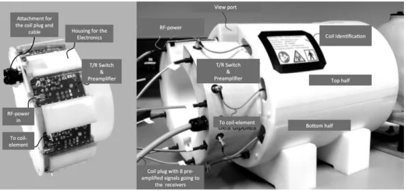
3.4 Transmit-Array Coil . . . 40
3.5 Computational Resources . . . 43
4 Specific Absorbtion Rate Assessment 45 4.1 Introduction. . . 46
4.2 Part I: Validation of Electromagnetic Simulations . . . 46
4.3 Part II: Online SAR Assessment Based on Time-Averaged Power Measurements. . . 51
5 Local SAR Reduction in Parallel Excitation Based on Channel-dependent Tikhonov Parameters. 57 5.1 Introduction. . . 58 5.2 Theory. . . 59 5.3 Methods . . . 59 5.4 Results. . . 62 5.5 Discussion . . . 65
6 kT-Points: Short Three-Dimensional Tailored RF Pulses for Flip-Angle Homogenization
Over an Extended Volume 67
6.1 Introduction. . . 68
6.2 Methods . . . 69
6.3 Results. . . 72
6.4 Discussion . . . 75
6.5 Conclusions . . . 77
7 Non-Selective Excitations with an Arbitrary Flip-Angle 79 7.1 Introduction. . . 80
7.2 Limitations of the (Extended) Small Tip Angle Approximation . . . 80
7.3 The Optimal Control Approach . . . 81
7.4 Adaptation to kT-points (with initial magnetization Mz= M0) . . . 84
7.5 Joint k-space optimization . . . 87
7.6 LTA pulse design: B+ 1 versus B0 . . . 90
7.7 Summary and Recommendations . . . 93
8 Parallel-Transmission-Enabled Magnetization-Prepared Rapid Gradient-Echo T1-Weighted Imaging of the Human Brain at 7 Tesla 95 8.1 Introduction. . . 96
8.2 Methods . . . 97
8.3 Results. . . 99
8.4 Discussion . . . 107
8.5 Conclusions . . . 109
9 A Minimalistic approach to Transmit-SENSE 111 9.1 Introduction. . . 112
9.2 Methods . . . 112
9.3 Results. . . 115
9.4 Discussion . . . 118
10 Summary & Recommendations 121
Bibliography 123
Les hauts champs magnétiques constituent une solution prometteuse
dans la poursuite d’une résolution toujours plus fine des images IRM.
Alors que la montée du champ statique améliore progressivement le
signal RMN (
Ocali and Atalar
,
1998
), elle augmente simultanément
la fréquence de Larmor des protons. Si on considère les systèmes
clin-iques à 3 Tesla, la longueur d’onde RadioFréquence (RF) est déjà
com-parable aux dimensions transverses du corps humain. En conséquence,
lors d’investigations sur les grands organes tels que l’abdomen ou les
cuisses, des zones d’ombre et des pertes de contraste faussent l’image
(
Bernstein et al.
,
2006
). En passant à 7 Tesla, les disparités de
ré-partition spatiale du champ RF sont si fortes que les artefacts de
contraste se développent aussi dans des régions plus petites telles que
le cerveau humain. Dans la perspective des premiers systèmes à 11.7
Tesla actuellement en cours de réalisation à NeuroSpin et au NIH, il
de-vient crucial de fournir des solutions pour atténuer les non-uniformités
de l’excitation des spins. A défaut de quoi, de tels systèmes à très haut
Pour relever ce défi, un système de transmission parallèle (pTx) à
8 canaux a été installé auprès de notre imageur à 7 Tesla. Alors
que la plupart des systèmes IRM cliniques n’utilisent qu’un seul canal
d’émission, l’extension pTx permet de jouer différentes formes
d’impulsions RF de concert sur plusieurs canaux. Si cette méthode
offre une grande souplesse dans la conception d’impulsions RF, elle
autorise également une pléthore de distributions d’énergie RF dans
le corps exposé (
Angelone et al.
,
2006
). Les dépôts d’énergie (Taux
d’Absorption Spécifique ou TAS) locaux et globaux devant être
lim-ités afin d’assurer la sécurité des patients (
IEC
,
2010
), il s’agit de
rechercher les formes d’impulsions RF qui permettront d’exciter le
motif désiré sans introduire de « points chauds ».
Les degrés de liberté supplémentaires fournis par l’extension pTx
peu-vent être mis à profit pour orienter la solution RF vers des distributions
d’énergie favorables. Dans ce travail de thèse, cette considération est
démontrée par l’optimisation itérative d’un ensemble de paramètres
les points chauds (
Cloos et al.
,
2010c
). On montre que si cette
ap-proche intuitive est robuste et gérable sur le plan computationnel, elle
impose en revanche une légère dégradation de la fidélité d’excitation
en général. Des méthodes récentes plus élaborées ont été publiées
permettant à la solution RF d’être optimisée vis à vis du TAS, tout
en conservant un niveau de fidélité fixe (
Brunner and Pruessmann
,
2010
;
Lee et al.
,
2010
). Cependant, ces méthodes sont encore
lim-itées à l’approximation des petits angles de bascule de l’aimantation
(
Pauly and Nishimura
,
1989
). Compte tenu de la robustesse et de la
flexibilité offerte par l’approche du contrôle optimal (
Xu et al.
,
2008
),
les contraintes de TAS local et global pourraient être complètement
intégrées à la conception des impulsions RF même si des Angles de
Bascule (AB) élevés sont ciblés.
Au cours de cette thèse, la gestion du TAS local dans la
concep-tion d’impulsions RF a été principalement un exercice théorique pour
illustrer la flexibilité de l’approche pTx. En effet, jusqu’à présent,
rité RF installés, la phase et l’amplitude transmises n’étant pas
surveil-lées en temps réel sur chaque canal, ce qui oblige à considérer la pire
des interférences de champ électrique en chaque instant et en chaque
voxel. Même si une approche pratique de l’évaluation en ligne du
TAS ainsi surestimé a été mise en œuvre, cette méthode
conserva-trice ne permet pas d’exploiter les véritables et souhaitables
inter-férences destructives du champ E. Par conséquent, l’optimisation du
vrai TAS local ne fournit que des avantages limités dans ce cadre de
travail bridé. Cependant, des systèmes de surveillance de TAS plus
sophistiqués finiront par rendre possible les bénéfices de la conception
d’impulsions sous contrainte de TAS local (
Graesslin
,
2008
;
Gagoski
et al.
,
2009
). Notre approche conservatrice a néanmoins permis de
valider de nouvelles stratégies de conception d’impulsions in-vivo.
La conception d’impulsions RF non-sélectives de type « k
T-points »,
introduite dans ce travail pour homogénéiser l’AB sur des volumes
étendus, est largement testé dans le contexte de la pTx en imagerie
est de limiter la trajectoire de l’espace-k de transmission (parcourue
avec les gradients) à un petit groupe de points autour du centre de cet
espace. De cette façon, comme les inhomogénéités RF sont dominées
par de basses fréquences spatiales, la limitation des excursions dans
l’espace-k garantit qu’aucune énergie n’est gaspillée à des fréquences
spatiales élevées d’un faible intérêt pour l’uniformisation de l’AB. De
plus le temps requis pour couvrir les quelques k
T-points est minimisé,
permettant une faible durée des impulsions simultanées résultantes.
En définitive, le véritable test de la stratégie des k
T-points est
démon-tré par sa capacité à regagner un excellent contraste entre les tissus
cérébraux au cours de séquences 3D traditionnelles comme la
MP-RAGE (
Mugler and Brookeman
,
1990
). En généralisant la conception
d’impulsions RF à des impulsions à grand AB (inversions) grâce à
l’approche du contrôle optimal, les impulsions adiabatiques
gourman-des en TAS peuvent être remplacées par gourman-des impulsions basées sur
les k
T-points plus efficaces et moins énergivores, restorant le contraste
Ainsi ces inversions, rendues possibles par la pTx, améliorent
simul-tanément la qualité d’image, le TAS déposé, et ce avec une durée
d’impulsion réduite. Les effets de susceptibilité magnétique, qui
aug-mentent avec le champ statique, peuvent toutefois représenter un défi
aux impulsions d’inversion basées sur les k
T-points. Bien qu’on
mon-tre que ces effets peuvent êmon-tre mitigés si on prend en considération
les régions touchées dans la conception des impulsions, la qualité du
résultat final dépend grandement de la précision avec laquelle la
ré-gion d’intérêt (ROI) est démarquée. En ce qui concerne les
applica-tions en neuro-imagerie, des logiciels dédiés sont disponibles pour
ex-traire le volume du cerveau à partir d’images de qualité. Cependant,
quand on définit la ROI pour la conception d’impulsions, de telles
images ne sont pas encore disponibles. Ainsi, de tels programmes
doivent s’accommoder d’images faiblement contrastées avec une
réso-lution grossière, pour lesquels ils ne sont pas optimisés. Malgré ces
processus de démarcation de ROI, cependant que des améliorations de
robustesse sont encore désirables.
Dans le travail présenté ici, seules des séquences de type Echos de
Gradients sont considérées. Pour étendre la portée des k
T-points aux
séquences de type Spin-Echo, l’algorithme de conception devrait être
généralisé pour inclure les impulsions refocalisantes. Des premiers
jalons ont été posés dans ce sens, de sorte à pouvoir incorporer de
telles impulsions dans des séquences 3D comme la SPACE (
Mugler
et al.
,
2000
).
Si on observe plus en détail notre conception d’impulsions RF à grand
AB, l’approche de contrôle optimal commence avec une solution
ini-tiale basée sur l’approximation des petits angles. Cependant ceci
im-pose des limitations sévères sur la solution optimisée : le minimum
local de la fonction de coût trouvé n’est pas garanti proche du
min-imum global. Par ailleurs, l’inclusion de la trajectoire de l’espace-k
comme sous-ensemble de paramètres au sein de l’optimisation fait de
tuitivement, il semble qu’en améliorant la conception d’impulsions à
grand AB, le dépôt d’énergie pourrait être encore plus réduit.
Finalement, l’implémentation de la pTx elle-même est reconsidérée
dans cette thèse. Bien que nous ayons pu montrer d’excellents
résul-tats avec une extension à 8 canaux, les coûts et l’expérience technique
nécessaires pour exploiter un tel système posent problème pour un
us-age en routine clinique. Par conséquent plusieurs configurations
sim-plifiées sont envisagées par le biais de la simulation, pour évaluer le
potentiel d’une solution hardware à moindre coût avec un nombre
ré-duit de canaux de transmission. De premiers résultats montrent que,
au moins dans le régime des petits angles de bascule, deux canaux
parallèles (ou mêmes séquentiels) sont suffisants pour homogénéiser
l’AB dans le cerveau humain à 7T. Pour le moment, ces résultats sont
basés sur des cartes de B
+1
mesurées in-vivo avec notre système pTx à
8 canaux. Une des étapes suivantes est de réaliser le hardware
capa-ble de piloter une antenne à N éléments de transmission en utilisant
l’applicabilité de cette approche dans un environnement clinique, ce
concept devrait être évalué sur d’autres parties du corps humain et en
considérant tous les AB possibles. En particulier, pour chaque
appli-cation clinique particulière, les limitations en termes de TAS devraient
être investiguées pour déterminer si un système à 2 canaux est
suff-isant ou si davantage de voies sont requises au regard de la fidélité
d’excitation désirée.
Medical imaging concerns a wide variety of methods dedicated to aid the diagnostic process and further the understanding of pathological conditions. From the perspective of both patient comfort and clinical perfor-mance, in particular when considering delicate anatomical structures with limited regenerative capabilities such as the brain, non-invasive techniques are often preferable. Although neuroplasticity facilitates some structural reorganization to mitigate the impact of lesions (Cao et al., 1994; Buonomano and Merzenich,
1998), recent studies suggest that the vast majority of neurons in the human neocortex are created at a prenatal stage and persists throughout most of each individual’s life without replacement (Nowakowski,
2006).
Over the years, several tomography methods have been developed to provide clinically relevant brain images (Abraham, 2011). Among the most well known three-dimensional imaging techniques to date are: Com-puted Tomography (CT), Positron Emission Tomography (PET) and Magnetic Resonance Imaging (MRI). Although each of the aforementioned techniques has its merits, the first two of them both involve ionizing radiation and offer either limited soft tissue contrast or a relatively coarse resolution. On the contrary, MRI allows images to be resolved down to a sub-millimeter voxel size, while facilitating multiple contrast mech-anisms that can be exploited to differentiate between tissues or indicate various pathological conditions. In addition, functional MRI (fMRI) provides cognitive neuro-scientists with a window into the human mind. Considering the microscopic scale of the laminar and columnar structures in the cortex, there is a strong desire to perform measurements with high spatial and temporal resolution. Although planar multielectrode arrays (Strumwasser, 1958) and later linear multicontact electrodes (Barna et al., 1981) allow neural ac-tivation to be measured among neighboring columnar structures or different cortical layers, these invasive techniques are hampered by technical and ethical constraints. Apart from their limited spatial coverage, their tendency to result in glial scar formation limits their clinical applications and precludes them as in-vestigational devices for neuroscience concerning the healthy human brain (Cheung, 2007). What is more, none of these techniques offers the opportunity to provide the anatomical reference necessary to account for inter-subject morphological variability.
Magnetic resonance imaging, on the other hand, facilitates both the acquisition of functional data and the anatomical reference requisite for the averaging or comparison between multiple subjects (Friston et al.,
1995;Ardekani et al.,2005). Furthermore, highly-resolved structural brain imaging provides excellent tissue delineation, which has already provided profound insights into the ageing brain (Gur et al.,1991) and the progression of neurodegenerative diseases such as Alzheimer (Silbert et al., 2003) and Huntington’s disease (Thieben et al., 2002). Moreover, recent findings support the notion that various pathological conditions result in a regional-dependent deterioration of the cortical ribbon (Dickerson et al.,2009;Kirk et al.,2009). These findings have initiated a demand for high-quality highly-resolved cross-sectional and longitudinal studies focusing on isolated regions, such as the hippocampus (Breyer et al.,2010).
In pursuit of a MRI-based technique to satisfy the above-mentioned needs, ever-higher main magnetic field strengths are explored. In the 11 years since the introduction of the first 7-Tesla MRI system suitable for human imaging, close to fifty such ultra-high-field (UHF) systems, including several 9.4-Tesla systems, have been installed around the world. Combined with recent advances in phased-array-coil technology and sequence development, these UHF systems start to probe spatial resolutions comparable to those of the cytoarchitectonic structures in the brain (Yacoub et al., 2008; Von Economo and Koskinas, 1927). This allows cognitive neuroscientists to investigate the cortical activation with better spatial precision aiding them in their understanding of the processing and computations carried out by individual cortical columns (Grinvald et al.,2000).
However, already at 3-Tesla the radio frequency (RF) wavelength corresponding to the proton Larmor fre-quency becomes comparable to the dimensions of some imaged human body parts. This results in zones of shade and losses of contrast distributed across the images of large organs such as the abdomen or thighs (Bernstein et al., 2006). When migrating to 7-Tesla, dielectric resonances and RF interferences cause in-homogeneous excitation profiles to develop in the human brain (Yang et al., 2002; Van de Moortele et al.,
2005). Consequently, a sub-optimal signal-to-noise ratio is obtained and a strong bias introduced on the desired contrast, hampering tissue delineation with high confidence. With the first 11.7 Tesla systems now in active development at NeuroSpin and NIH, it becomes increasingly urgent to provide adequate solutions to mitigate these excitation non-uniformities so that these systems can reach their full potential.
Scientific goals addressed in this work
Although there are many technical challenges associated with UHF-MRI, this study focuses on the mitigation of excitation non-uniformities and restoring the desired contrast. Considering the origin of these artifacts (Yang et al.,2002), parallel transmission (pTx) is one of the most promising solutions available to eradicate these undesired effects. Originally proposed byKatscher et al.(2003) andZhu(2004), pTx utilizes multiple independently driven coil-elements to facilitate relatively short excitation pulses with the flexibility to obtain nearly any excitation pattern. However, there are certain risks inherent in this approach, stemming mainly from the potential occurrence of a highly localized energy deposition in the exposed volume. Therefore, special care must be taken to prevent tissue ablation. In spite of the fact that the relevant parameter is the RF induced temperature rise, for simplicity the specific absorption rate (SAR) is often considered instead. This measure of the energy deposition may then be constrained according to standardized guidelines (IEC,
2010) to provide adequate safety with respect to temperature (Massire et al.,2012).
While various interesting applications benefit from the enhanced degrees of freedom introduced by the pTx-approach (Setsompop et al.,2008a;Schneider et al.,2010;Katscher et al.,2010), the objective of this thesis is the development and demonstration of pTx-based techniques to provide substantial advances towards:
• High quality volumetric human brain imaging in UHF-MRI. • Specific absorption rate assessment and control.
Overview of this thesis
First the fundamental concepts of MRI are introduced in chapter 1, concluding with the advantages and challenges encountered at UHF. Subsequently, the concepts and techniques particular to the pTx approach are detailed in chapter 2, followed by an overview of the experimental setup (chapter3) used throughout the succeeding chapters. Because SAR management is essential to perform in-vivo experiments, we present in chapter 4an progression of SAR evaluation methods that allowed along the course of this thesis to gain latitude in RF pulse design and in MRI exams. The rest of this manuscript is devoted to radio-frequency pulse design. After presenting an original approach to iteratively minimize the local SAR by penalizing different transmit-pathways (chapter 5), a new strategy named “kT-points” for non-selective excitations
achieving excellent flip angle homogenization over the whole brain is demonstrated in chapter6. Encouraged by the small-tip-angle results and low energy excitations, its application to the large flip-angle regime is investigated by combining it with optimal control theory (chapter7). Ultimately, and via the progress made in SAR assessment, the method was tested in the MP-RAGE (Mugler and Brookeman, 1990), one of the most commonly used T1-weighting 3D sequences. The results of in-vivo experiments at 7 Tesla presented in
chapter8prove the viability of the technique as well as good mitigation of the RF and B0-field inhomogeneity
artifacts for this sequence. Finally in chapter9, simplifications in the global design of the pTx-implementation are studied to investigate more cost-effective solutions and more manageable SAR scenarios. Chapter 10
concludes this thesis with a summary of the most substantial scientific contributions and a brief outlook on possible future developments.
1.1
Nuclear Magnetic Resonance
Most particles have, besides classical properties such as mass and charge, an intrinsic property referred to as spin1. This quantum mechanical property endows each of the nucleons with a spin value of1/
2. Although
nuclei can be comprised of multiple nucleons, it turns out that the simplest configuration, the Hydrogen proton, is the most abundant spin1/2nucleus in organic tissues.
When immersed in a static magnetic field (B0) oriented along the z-axis, the Hamiltonian matrix
corre-sponding to the resulting potential energy is:
H = −γB20~σz= −γB0 ~ 2 ✓ 1 0 0 −1 ◆ (1.1) where γ is the gyromagnetic ratio (γ
2π = 42.6 10
6Hz T−1 ), ~ is Planck’s constant divided by 2π, and σ z is
Pauli’s spin matrix matching the selected direction of the magnetic field (Griffiths,1994). The corresponding eigenstates are: χ− with energy : E−= −γB0~ 2 χ+ with energy : E+= +γB0 ~ 2 (1.2) where χ− is the lower energy state co-aligned with the main magnetic field, and χ+ the anti-aligned state.
Consequently, this system could interact with a (virtual) photon of energy γB0~, corresponding to a frequency
of:
ν = E−− E+
2π~ =
γB0
2π , (1.3)
which is commonly referred as the proton Larmor frequency2.
Bloch Equations
Thus far, only a single particle was considered. All biological tissues contain many nuclei of which, in terms of body mass percentage, Hydrogen is the third most abundant in the human body (Zumdahl and Zumdahl,1999)3. The canonical ensemble of such spin1/2nuclei, when at thermal equilibrium immersed in
the above-mentioned static magnetic field, yields the following density of magnetization (Schroeder,1999) : M0eˆz=
ργ~
2 tanh (βE+) ˆez (1.4)
where ρ is the proton spin-density, β def= (kT )−1 is defined as the reciprocal of the Boltzmann’s
con-stant times the temperature in Kelvin4. When perturbed by an RF-field, the magnetization vector M = {Mx(t), My(t), Mz(t)}T obays the Bloch equation:
∂ ∂tM= −γB ⇥ M − 0 @ 1/T2 0 0 0 1/T2 0 0 0 1−M0/Mz T1 1 A M (1.5) 1
The interpretation of spin is by no means trivial; for those who are interested the author recommends a most intriguing article byOhanian(1986).
2
Strictly speaking, real photons do not constitute the dominant energy quanta considered in the context of MRI. It has been suggested that the virtual photons often considered in quantum field theory are more fitting. More background regarding these considerations can be found in (Hoult and Bhakar,1997).
3
Oxygen is first followed by Carbon, both of which, in their natural abundant form, have an effective spin of 0.
4
Most textbooks on NMR emphasize on the first order Taylor expansion: M0eˆz≈ργ
2~2
where B = {Bx(t), By(t), Bz(t)}T is the magnetic field which may depend on time and whose static main component remains oriented along the z-axis, T1 is the longitudinal relaxation time, and T2 the transverse
relaxation time (Bloch, 1946; Wangsness and Bloch, 1953). Instead of describing the magnetization from the perspective of an observer in the laboratory frame of reference, it is often more convenient to consider the transverse and longitudinal magnetization in the frame rotating at the Larmor frequency Ω = γB0. To
this end, the transformation matrix: Λ(Ωt) = SR(Ωt) = 0 @ 11 −i 0i 0 0 0 1 1 A 0
@ cos (Ωt)sin (Ωt) − sin (Ωt) 0cos (Ωt) 0
0 0 1
1
A (1.6)
can be used to carry the observer into a more convenient frame of reference. Defining ˜M = Λ(Ωt)M = '
MT(t) , MT(t) , Mz(t) T
(where MT(t) = Mx˜(t)+iMy˜(t), MT(t) = Mx˜(t)−iMy˜(t), and Mx˜(t) & My˜(t)
are the Cartesian magnetization components in the rotating frame), B˜ = Λ(Ωt)B
def
= nB+1 (t) , B1+(t) , B0+ ∆B0
oT
(where, after neglecting the off-resonance components (Hoult, 2000b)5, 2B1+(t) ⇡ Bx˜(t) + iBy˜(t) and Bx˜(t) & B˜y(t) are the Cartesian magnetic field components in the
rotat-ing frame, and ∆B0 accounts for localized deviations from the static magnetic field B0 ), and exploiting
]
[B]⇥ = Λ (Ωt) [B]⇥Λ−1(Ωt)( where [B]⇥ is a matrix such that [B]⇥M= B ⇥ M (Jaynes, 1955)), allows Eq. 1.5to be rewritten as:
∂ ∂tM˜ = −iγ 0 B @ MT(t) ∆B0− MzB1+(t) 0 MT(t)B + 1(t)−MT(t)B + 1(t) 2 1 C A | {z } ”Conventional description” + iγ 0 @ 0 MT(t) ∆B0− Mz(t) B+1 (t) 0 1 A | {z } ”Conjugate description” − 0 @ MT(t)/T2 MT(t)/T2 Mz(t)−M0 T1 1 A | {z } Relaxation . (1.7)
According to these definitions, the first two rows of equation 1.7 both describe the time-evolution of the transverse magnetization. Therefore, traditionaly, the ”Conjugate description” is disregarded in favor of a more concise expression6. Consequently, the co-rotating component of the magnetic field (B+
1) constitutes
that component of the transmit-field suitable to introduce a transverse component (MT) in to the
magne-tization vector. In the context of NMR, the flip-angle (FA or θ) is often adopted to express the result of a B1+ excitation: θ = γB+1
´T
0 f (t) dt, where T is the duration and f(t) is the pulse shape. If the initial state
of the magnetization is M0eˆz, and Mz is the longitudinal component after the excitation, then:
θ = arccos ✓ Mz kMk ◆ . (1.8)
T
1Relaxation
The longitudinal relaxation time T1 is a tissue-specific characteristic constant related to the time required
for the substance in question to (re-)establish its net thermal equilibrium magnetization. This can be seen when considering the immersion of the object into the main magnetic field at t = 0:
∂
∂tMz= −
Mz− M0
T1
, (1.9)
which has the solution:
Mz(t) = M0
⇣
1 − e−t/T1⌘
. (1.10)
During this process, energy is transferred to the spin-lattice as the population of the eigenstates is changed (Eq. 1.2). This characteristic time constant is inversely proportional to the efficiency at which energy can be dissipated to other nuclei in the lattice.
5
Hence the factor 1/2 in: B1+(t) ≈B˜x(t)+iBy˜(t)
2 . 6
Note that B1+should not be confused with B−
1 which is related to the receive sensitivity, i.e., it contains no additional
T
2Relaxation
The transverse relaxation time T2 is a measure of how long the resonating protons remain coherent, i.e.
in phase, following an excitation. Considering a simplified model where only the transverse component is considered: ∂ ∂tMT = − MT T2 , (1.11)
the following solution is found:
MT(t) = MT(0) e−
t/T2
, (1.12)
where MT(0) is the transverse component at t = 0. The resulting decay in transverse magnetization is
due to magnetic interactions occuring between protons. For example, neighboring protons bound to macro-molecules locally change the magnetic field sensed by the free protons. These local field non-uniformities cause the free protons, which constitute the dominant component in the MR signal, to precess at slightly different frequencies. Thus, following an excitation pulse, the protons lose coherence and the net transverse magnetization is gradually lost.
The NMR signal
The previous sections briefly explained how an ensemble of protons immersed in a magnetic field may be excited, and the mechanisms that allow it to relax back to equilibrium. However, in order to exploit this behavior in the framework of NMR, a measurable signal needs to be extracted. To this end, let us consider a Hertzian loop placed close to the sample and prependicular to the transverse plane. Following an ideal 90◦ excitation, the magnetic moment precesses in the xy-plane (at the Larmor frequency). The rotating
magnetic field of the nuclear magnetization induces an electromotive force (EMF) in the loop, much like a bicycle dynamo (Hoult and Bhakar,1997). Since the induced EMF is proportional to the field produced by the oscillating magnetic moment, a suitable analog-to-digital converter (ADC) may be used to observe the time evolution of the system and facilitate subsequent computerized post-processing. Because the current induced in the Hertzian loop (or a more optimized receive-coil) is directly proportional to the transverse magnetization, the loss of coherence due to T⇤
2 relaxation will result in the recording of an attenuating
signal7. This measurement corresponds to what is referred to as the free induction decay (FID) (Hahn,
1950a).
1.2
Magnetic Resonance Imaging
Historic introduction
Originally only published in a PhD thesis, the first transitional steps from NMR to MRI were pioneered by
Carr (1952). This was later extended byLauterbur, P.C. (1973) to produce the first 2D images, followed by the first cross-sectional image of a living mouse (Lauterbur, P.C., 1974). These experiments were still performed using a standard NMR spectrometer with an added field gradient, thus introducing the concept of frequency encoding. In the absence of a magnetic field gradient, the Fourier transform of the FID results in a peak corresponding to the Larmor frequency of the sample (Fig. 1.1a). When a linear gradient is applied, multiple frequencies are introduced into the FID dependent on the location of the source. Consequently, the Fourier transform now corresponds to the spatial distribution of the sample along the direction of the field gradient (Fig. 1.1b). Although this 1D technique was a milestone in the development of MRI, this first implementation was far from practical. Considering the fixed nature of the field gradient in these experiments, the object under investigation had to be physically rotated to resolve a two-dimensional image. Much faster imaging techniques involving multiple linear field gradients were pioneered by Kumar et al.
(1975);Mansfield and Maudsley (1976);Mansfield(1977). These techniques resemble more closely to what is now common practice, rather than the projection technique originally used by Lauterbur, P.C. (1974). Current clinical MRI systems provide time variable linear magnetic-field gradients in three orthogonal di-rections (Fig. 1.2) to allow 2D- and 3D-Fourier-transform based spatial encoding techniques.
7
The measured attenuation corresponds to the time constant T⇤
2, which incorporates the loss of coherence due to T2
Figure 1.1: Frequency encoding in MRI. a: Three compartments filled with water immersed in a static magnetic field B0 result in a FID whose spectrum shows the Larmor frequencies present in the sample, e.g., a single proton peak in this case. b: Three compartments filled with water immersed in a linear field gradient on top of a static magnetic field B0 result in a FID whose spectrum is the projection of the sample along
the direction of the linear field gradient.
Figure 1.2: Schematic overview of the basic coil configuration in current MRI systems. 1: The main magnet responsible for the static magnetic field in the z-direction (B0). Nowadays this typically entails a
superconducting magnet cooled with liquid helium (Minkoff et al.,1977). 2: Gradient coils used to produce linear field gradients along the x and y direction through the subject (in a limited region of interest). 3: Gradient coils used to produce linear field gradients along the z-axis. 4: Head coil used for RF excitation and NMR signal reception. Many clinical systems are also equipped with a larger RF transmission coil for whole body applications (not shown), comparable in size to the gradient coil diameter. 5: Subject. 6: Patient table.
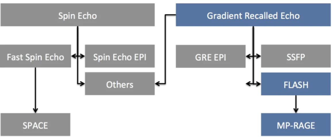
Figure 1.3: Schematic overview of the basic pulse sequences in MRI. Spin Echo (Hahn, 1950b), Fast Spin Echo (Feinberg et al.,1985b), Echo Planar imaging (EPI (Mansfield,1977)), SPACE (Mugler et al.,2000), Gradient Recalled Echo (GRE), Steady-State Free precession (SSFP (Oppelt,1986))), Fast Low Angle Shot (FLASH, (Haase et al., 1986)), Magnetization-Prepared RApid Gradient Echo (MP-RAGE, (Mugler and Brookeman, 1990)), Others (Bernstein et al., 2004; Haacke et al.,1999).
Current Imaging Sequences
Over the years, numerous imaging methods have been introduced, commonly referred to as acquisition sequences. Loosely speaking, two classes of sequences exist, the Gradient-Recalled-Echo (GRE) and the Spin-Echo (SE) branches (Fig. 1.3). Stepping over many important advances in the field8, only those sequences most relevant to the work presented in this thesis will be considered in more detail (Fig. 1.3, Blue). First the GRE is explained in the context of a volumetric acquisition. Then the FLASH sequence is presented in the framework of slice selective excitation. Finally the Magnetization-Prepared RApid Gradient Echo (MP-RAGE) sequence, one of the most commonly used methods to obtain T1-weighted images of the
whole brain, is summarized.
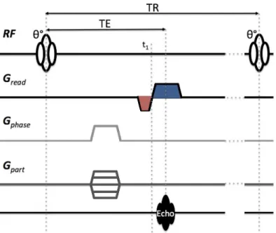
Gradient Echo and 3D imaging
Rather than adopting a fixed field-gradient for frequency encoding, it is often more convenient to consider a field echo. This may be accomplished using two gradient lobes (Fig. 1.4, red & blue). First the prephasing lobe (Fig. 1.4, red) dephases the transverse mechanization such that the subsequent readout lobe with opposite polarity (Fig. 1.4, blue) refocuses the spins to produce the desired echo.
Mathematically, this can be seen as follows: after an excitation, the prephasing gradient introduces a spatial dependence (r) to the precession frequency:
ω (r, t) = γ (B0+ Gpre(t) · r) (1.13)
where Gpre(t) is the gradient waveform during prephasing. Therefore, in the rotating frame of reference,
the relative phase accumulated during the prephasing gradient is: φpre(r, t) = γ
ˆ t
0
Gpre(t) · r dt . (1.14)
Neglecting relaxation effects and assuming a spin density distribution ρ(r), the following expression for the signal just after the prephasing gradient (t = t1) is obtained:
S (t1) = γ sin (θ)
ˆ 1
−1
ρ (r) e−i2πkpre(r) d3r (1.15)
8
For a more complete overview of the different imaging techniques, the reader is directed to one of the numerous textbooks such as (Bernstein et al.,2004;Haacke et al.,1999).
Figure 1.4: Schematic overview of the basic gradient recalled echo sequence. (The prephasing gradients, including phase an partition gradient lobes, may be played at the same time to allow shorter echo times.) where kpre(r)
def
= 1
2πφ(r, t1)is the k-space offset, and θ is the flip angle produced by the excitation. In order
to obtain the desired echo centered on the readout gradient lobe Gread(t), the following conditions need to
be satisfied: ˆ T E t1 Gread(t) · r dt = ˆ t1 0 Gpre(t) · r dt (1.16)
where TE is the time of echo commonly specified relative to the center of the excitation (Fig. 4). Consid-ering a GRE-based sequence, the prephase and imaging gradient lobes may be concatenated into one single continuous gradient waveform (Fig. 1.4).
To illustrate more clearly the Fourier relation between the signal and spatial distribution of the spin density, consider the following substitution:
ˆ
ρ (r) = ρ (r) e−2πikpre(r) . (1.17)
Assuming that the gradient is constant during the readout, we can rewrite the signal corresponding to the echo as:
SEcho(t) = γ sin (θ)
ˆ 1
−1
ˆ
ρ(r)e−γiGread·rtd3r, (1.18)
which simply constitutes a one-dimensional Fourier-transform of the spin density. However, so far, only a projection of the image along the read direction of Greadcan be obtained, whereas the other two directions are
just integrated. In theory it is possible to reconstruct the entire volume by acquiring multiple projections along different directions. More commonly, the full k-space is acquired with the aid of phase encoding gradients (Fig. 1.4, gray). Including these phase encoding gradient lobes we find:
SEcho(t, u, v) = γ sin (θ)
ˆ 1
−1
ρ(r)e−2πikpha(r)ue−2πikpart(r)ve−2πikpre(r)e−γiGread·rtd3r (1.19)
where u and v are repetition-dependent scaling factors of the maximum k-space excursions (kpha, kpart)
orthogonal to one another and the read direction (Gread). Iterating this strategy with a time of repetition
TR, allows k-space to be sampled uniformly and the spin density distribution ρ (r) to be recovered via the 3D Fourier transform. However, when implemented on a physical scanner, the temporal signal has to be discretized (sampling), and images have to be reconstructed adopting the discrete Fourier transform. Moreover, additional system limitations such as gradient amplitude, gradient slew-rate, and ADC bandwidth have to be taken into account when building an acquisition sequence (Bernstein et al.,2004;Haacke et al.,
Figure 1.5: Schematic overview of the basic FLASH sequence. Fast Low Angle Shot and 2D imaging
The basic GRE sequence described in the previous section assumes the initial magnetization prior to any RF pulse is longitudinal in all voxels. This is true if TR is very long compared to the T2 of the sample.
When the TR becomes comparable or shorter than T2, unwanted stimulated echoes may arise9, corrupting
the final image. This poses a problem for most clinical applications as the total scan time would become too long. To allow high-quality images with a short TR, some modifications to the basic GRE sequence are necessary (Fig. 1.5).
In order to circumvent unwanted stimulated echoes, the spoiler gradient (Fig. 1.5, blue) combined with incremental quadratic RF phase shifts are introduced (Haacke et al.,1999;Bernstein et al.,2004). The idea behind the spoiler gradient is to dephase the spins inside every voxel so that no transverse magnetization is left when restarting RF transmission. Considering a voxel of size ∆r, the minimum necessary gradient envelope is:
γ ˆ
Gspoil(t) · ∆r = 2π . (1.20)
In addition to the spoiler, re-winder gradient lobes are generally introduced (Fig. 1.5, green). These additional lobes are the exact opposite of the phase encoding gradients, restoring the spin coherence in the phase encode directions10.
While the spoilers destroy the spin-coherence at the end of the TR, the longitudinal component of the magnetization remains untouched by them. After several repetitions, this leads to a steady state where T1
relaxation and excitation effects stabilize. Then the following steady state signal equation applies: S (T R, T E , θ) / sin (θ) ρ (r)
3
1 − e−T R/T14
1 − cos (θ) e−T R/T1e
−T R/T ∗2 , (1.21)
which allows the Ernst angle corresponding to the maximum signal for a given TR to be calculated via: θE = arccos
⇣
e−T R/T1⌘ . (1.22)
Thus, for very short TR, the maximum signal will be reached for a small FA.
Although this sequence can be used to obtain volumetric images, as described in the previous section, the example depicted in Figure 1.5illustrates the principles of a 2D image acquisition. The rationale is to limit
9
Stimulated echoes can occur due to the refocusing of magnetization initialized by RF exposure in earlier repetitions, i.e., magnetization created more than n × T R + T E (n ∈ N ) ago. These echoes do not necessarily result in an artifact, some sequences use this to their advantage (Oppelt,1986;Mugler et al.,2000).
10
Figure 1.6: Schematic overview of one TRm of the MP-RAGE sequence. Orange: Magnetization preparation (MP) element including a non-selective inversion followed by a spoiler. Green: FLASH-based readout for a single k-space partition. TI: Time of Inversion, defined from the center of the inversion pulse to the center of the k-space partition in the FLASH train. TRm: the time between consecutive inversion pulses.
the excitation to a single slice through the volume, such that the integrated signal in the direction orthogonal to the slice is limited to the slice profile itself. To this end, a gradient of amplitude G is applied during the RF pulse (Fig. 1.5, red) to introduce a spatial linear dependency in the Larmor frequency distribution (Eq. 1.13). Combined with an RF-pulse of limited bandwidth (BW), a single slice with a finite thickness is excited. However, during this slice selection gradient, the transverse component of the spins is dephased along the slice profile. Therefore, a second gradient lobe with opposite polarity and half the time integral is concatenated after the RF pulse to restore coherence. The slice selection eliminates the necessity for partition encoding and allows the image to be reconstructed with a 2D Fourier transform. Nevertheless, the principle of slice-selective excitation can also be paired with volumetric imaging techniques to acquire a 3D slab through the exposed sample.
Magnetization-Prepared Rapid Gradient Echo
The magnetization-prepared rapid gradient echo sequence (Mugler and Brookeman, 1990), referred to as “MP-RAGE”, is among the most commonly employed 3D sequences to obtain T1-weighted anatomical
im-ages of the brain (Fig. 1.6). To this end, an inversion pulse is used (Fig. 1.6, orange) followed by a FLASH train (Fig. 1.6, green) acquiring one partition plane in k-space per repetition time TRm. Careful adjustment of the delay TI between the inversion and the acquisition block, as well as of the usual imaging parameters (θ, T R, T E), allows excellent contrast between gray matter, white matter, and cerebrospinal fluid (Deichmann et al.,2000;Mugler and Brookeman,1990).
1.3
Specific Absorption Rate
During an MRI exam, radio frequency waves are transmitted to acquire images of a subject. These RF waves deposit energy into the subject, resulting in an increase of temperature that could potentially lead to tissue damage. Therefore committees provide guidelines indicating the maximum allowed energy deposition in human subjects (IEC, 2010). These guidelines refer to the energy deposition as the specific absorption rate (SAR), given by :
SAR (r) = 1 T σ (r) 2ρ (r) ˆ T 0 kE (r, t)k 2 2 dt . (1.23)
This depends on the conductivity σ (r), the density ρ (r), the electric field distribution E (r, t) inside the subject, and the time of integration T during which instantaneous energy deposition is averaged.
The aforementioned guidelines refer to a set of 4 limits considering the maximum allowed energy deposition in the human head. These limits pertain to the global SAR, i.e. the SAR averaged over the entire head, and the local SAR, defined as the SAR averaged over any closed 10-g volume of tissue. The 4 limits provided by the guidelines consider both the T=10-second average and T=6-minute average. The following provides a summary of the SAR limits as defined for diagnostic experiments exposing the human head to an RF field:
• Guideline local SAR #1 • Guideline local SAR #2 • Guideline global SAR #1 • Guideline global SAR #2
30 W/kg per 10-s window of integration, averaged over any closed 10-g volume.
10 W/kg per 6-min window of integration, averaged over any closed 10-g volume.
9.6 W/kg per 10-s window of integration, averaged over the entire head. 3.2 W/kg per 6-min window of integration, averaged over the entire head.
In the case of human subjects, the exact fields and anatomical details are often unknown. As a result, the SAR cannot be determined with absolute accuracy for each individual. The conventional method for SAR assessment revolves around simulations based on subject models to estimate the global and peak local SAR. In order to provide secure operation, suitable 10-s and 6-min average power limits are derived for the RF transmitter to ensure compliance with the SAR guidelines.
1.4
Ultra High Field MRI
So far, the impact of the main magnetic field strength has not been considered in detail. However, both the signal-to-noise ratio (SNR) and contrast-to-noise ratio (CNR) are dependent on the field strength. In general the MR signal is proportional to:
SN R3D / M0B1−∆x∆y∆z
q
NphaseNparNreadNavrg
BW Sseq(T R, T E, θ)
SN R2D / M0B1−∆x∆y∆z
q
NphaseNreadNavrg
BW Sseq(T R, T E, θ)
(1.24) where M0 is the thermal equilibrium magnetization, B1− the receive sensitivity (RF magnetic field per unit
current in the receive coil), ∆x∆y∆z are the spatial dimensions of the voxels, Nphase the number of phase
encoding steps, Npart the number of partition encoding steps, Nread the number of samples in the readout,
Navrg the number of averages, BW is the readout bandwidth, and Sseq(T R, T E, θ) is a factor dependent
on the other sequence parameters11. Therefore, once receive coils and sequence parameters are adjusted to their optimal performance, the only options left to improve the MR signal are to increase M0 or decrease
the resolution. When high(er) resolution images are desired, the only remaining possibility is to increase magnetization. Looking back at equation 1.4, the net magnetization can be increased in two ways. Either the temperature of the object under investigation can be reduced, or the magnetic field can be increased12. Considering living biological tissues, significantly decreasing the temperature is not possible, leaving only the magnetic field strength as a free parameter.
Advantages
Apart from the direct improvement in SNR due to to an increased M0, pushing up the main magnetic field
strength brings other advantages. Most notably are the enhanced T⇤
2 contrast, and performance boost when
adopting parallel imaging methods (Sodickson and Manning,1997;Pruessmann et al.,1999;Griswold et al.,
2002).
11
In the case of a FLASH-based acquisition scheme, Sseq(T R, T E, θ) would be Eq. 1.21. 12
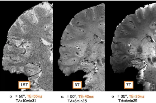
Figure 1.7: Comparison of the contrast-to-noise ratios, comparing gray matter and white matter, obtained at different field strengths on a coronal slice through the brain. All images were acquired with a T⇤
2-weighted
sequence and quadrature head coil. Comparing T⇤
2-weighted images obtained at different field strengths, a substantial improvement in CNR
can be obtained when migrating from 1.5 to 7 Tesla (Fig. 1.7). This increased T⇤
2 contrast is not only
beneficial for structural brain imaging. Considering BOLD-based fMRI for example, the physiological noise contributions (veinous blood) are expected to decrease with increased resolutions while the BOLD signal increases with field strength (Triantafyllou et al.,2005).
In general, it is desirable to constrain the acquisition time to a minimum, not only because of patient comfort and cost efficiency, but also to minimize motion artifacts. As the acquisition time becomes longer, it becomes increasingly difficult for the subject to refrain from moving. Furthermore, even small artifacts due to involuntary movements such as swallowing and breathing can be problematic when considering ultra-high-resolution structural imaging. Moreover, in the context of probing the microscopic scale of the laminar and columnar structures in the cortex, even brain movement due to variations in the cerebral spinal fluid pressure (Maier et al.,1994;Alperin et al.,1996) is a potential source of artifacts.
Parallel imaging (Sodickson and Manning, 1997; Pruessmann et al., 1999; Griswold et al., 2002) is one of the most potent tools available to decrease the acquisition time while maintaining contrast and resolution. This technique exploits the different sensitivity profiles from multiple receive elements (Roemer et al.,1990) to reconstruct an under-sampled image. The key principle behind these methods is the approximate or-thogonality between the different receive sensitivities. With increased field strength, therefore shortened RF wavelengths, the receive profiles corresponding to each of the coil elements become more distinct. Conse-quently, higher acceleration factors can be reached with only limited image quality degradation (Ohliger and Sodickson, 2006).
Challenges
Alongside the opportunities provided by UHF-MRI, several challenges arise. As the external field (B0)
increases in strength, so does the induced magnetization (M = χmH). Consequently, in those boundary
areas where the difference between susceptibility constants (χm) is large, such as the air-tissue interface,
substantial fluctuations are introduced into the static field observed by the spins. Due to the dependence on the external field, these non-uniformities become more pronounced in UHF-MRI. Although the bulk of these effects can be compensated with the aid of first and second-order shim coils, residual variations typically remain near intracranial cavities. These undesired disparities in the main field not only result in signal loss due to intravoxel dephasing, but also in geometrical distortions originating from the bias introduced in the frequency encoding. Looking back at the comparison shown in Figure1.7, the appearance of an increasingly
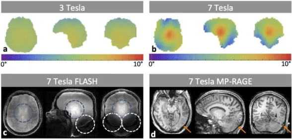
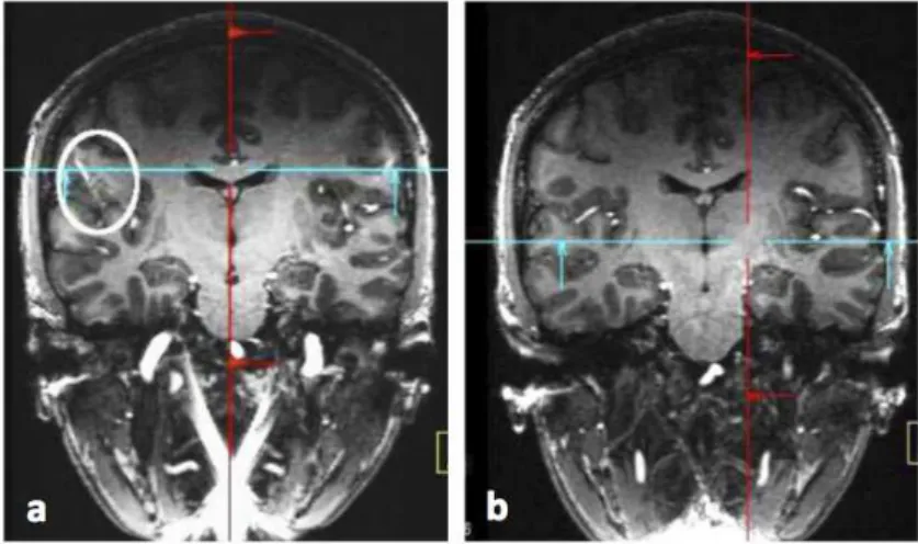
Figure 1.8: Comparison of the excitation uniformity obtained at 3 and 7 Tesla. a: Map of the flip-angle distribution obtained at 3 Tesla (Siemens Magnetom Tim Trio). b: Map the flip-agle distribution obtained at 7 Tesla (Siemens Magnetom, equipped with a home-built RF-coil). c: Image acquired with a FLASH sequence at 7 Tesla (equipped with a quadrature head coil). Blue rings indicate what is commonly referred to as the central brightening effect, whereas the white rings indicate the areas of signal loss. d: Image acquired with the MP-RAGE sequence at 7 Tesla (home-built RF-coil). Orange arrows indicate the approximate area where the contrast between gray and white matter is lost.
large cavity can be seen at the bottom of the temporal lobe. Although there may be some subject variability involved, to first order, this deviation is due to increased magnetic susceptibility effects introduced by the inner-ear proximity. Interestingly, the thriving potential of parallel imaging at UHF can in some cases be adopted to mitigate these geometrical distortions and signal losses (Weiger et al.,2002).
Apart from the increased sensitivity to magnetic field susceptibilities, UHF-MRI is hampered by an increased level of excitation non-uniformity (Fig. 1.8a & b). Although these effects are a hot topic with respect to current endeavors in UHF-MRI, Bottomley and Andrew in 1978 already predicted their impact on MRI. Looking back at the signal equation of the FLASH sequence (Eq. 1.21), it becomes apparent that a spatial variation of the FA will introduce unwanted contrast variations (Fig. 1.8c). Although this is just one example, various techniques, such as the MP-RAGE and SPACE sequence, are even more sensitive to these variations (Fig. 1.8d).
Besides the increased non-uniformity of the excitation field,Bottomley and Andrew(1978) also predicted an increased energy deposition. Considering the idealized case of a homogeneous spherical phantom centered in a quadrature coil, the following relation between absorbed power (W ) and angular-frequency (ω = γB0)
is found (Hoult and Lauterbur, P.C.,1979;Hoult,2000a): W = 2πω
2B+2 1 a5
15 (1.25)
where a is the radius of the sphere. Targeting a certain FA, for a fixed pulse duration the B+
1-field necessary
to yield it is independent of the main magnetic field strength B0. Although there are some correction
terms for the above-presented equation at high frequencies (Hoult,2000a), it clearly illustrates the quadratic relation between global SAR and B0. Moreover, depending on the setup at hand, the maximum local-SAR
to global-SAR ratio may increase as a result of the reduced wavelength and enhanced interference effects. Consequently, certain SAR-demanding imaging protocols commonly adopted at low field strength need to be reconsidered before application at UHF.
2.1
A k-space analysis of small-tip-angle excitations
Much like the slice-selective excitation introduced in the previous chapter, tailored pairs of RF and gradient waveforms may be employed to selectively excite nearly any excitation pattern. Drawing an analogy to the Fourier encoding used in the imaging processes, the concept of k-space can also be extended to the domain of multi-dimensional RF pulse design (Pauly and Nishimura,1989). This may be observed by studying the small-tip-angle (STA) approximation, which assumes that the longitudinal magnetization remains constant during RF exposure (Pauly and Nishimura, 1989). Indeed, when targeting a small flip-angle (FA , θ) and assuming an initial magnetization co-aligned with the static magnetic field, the transverse magnetization (MT) is proportional to sin(θ) ⇡ θ, whereas Mz remains approximately constant. Consequently, when
targeting a FA < 30◦ while neglecting both off-resonance and relaxation effects, the cumbersome non-linear
Bloch equation (1.7) can be linearized with the following approximation: ∂ ∂tMT(r) = −iγ 3 G(t) · r MT(r) − B1+(t)M0 4 (2.1) where G(t) and B+
1(t) are the time dependent gradient and RF waveforms, respectively. Solving this
differential equation for the final magnetization at time T results in: MT(r) = iγM0
ˆ T
0
B1+(t) e−ir·k(t)dt (2.2)
where, similar to the spatial frequency covered during image encoding (1.14), k(t) is defined as −γ ´tTG(s) ds.
Hence the “k-space interpretation” is found, where k(t) constitutes a trajectory through k-space correspond-ing to a set of pre-defined gradient waveforms (Pauly and Nishimura, 1989). Then MT(r) is the Fourier
Transform of the RF waveform as long as the latter is played while covering the whole k-space. Given a predefined trajectory, Equation 2.2 immediately suggests a multitude of spatially selective excitations to complement the earlier introduced slice-selective excitations. Considering the target MT(r) distribution
shown in Fig 2.1a, the RF-pulse corresponding to this excitation is simply the inverse Fourier transform of MT(r)(Fig2.1b) as it follows the Cartesian trajectory in Fig. 2.1c. This implies the RF-waveform is played
in concert with the gradients, resulting in an excitation with the desired characteristics (Fig. 2.1d). Albeit a powerful tool for spatial selection, most potential applications involving multidimensional RF pulses are hampered by hardware limitations. In particular, gradient slew-rate and amplitude constrain the minimal pulse duration due to the wide spatial-spectral range necessary to facilitate an arbitrary excitation profile. Although a judiciously chosen k-space design may be more favorable (Sersa and Macura, 1998), highly
Figure 2.1: Schematic overview of the different steps involved in the design of a single-channel Fourier-based small-tip-angle 2D pulse. a: The desired target magnetization. b: The RF-waveform corresponding to the Fourier-transform of target excitation pattern. c: Echo-planar (EP) k-space trajectory super-imposed in green on top of the Fourier-transform of the target magnetization. d: Final image after application of the designed RF + gradient waveforms in a suitable imaging sequence.
selective excitations generally still result in unacceptably long pulse durations. These may not only exceed the repetition time desired in many ultra-fast sequences, but also deteriorate image quality due to off-resonance, relaxation, and magnetization transfer effects during the pulse.
2.2
Transmit-Arrays
As mentioned in the previous chapter, the RF-inhomogeneity increases with field strength, progressively introducing a stronger bias in the acquired images. To mitigate these effects, transmit-arrays consisting of multiple independent coil-elements were introduced (Duensing et al., 1998;Ibrahim et al., 2001a; Adriany et al.,2005). In contrast to the phased arrays used for reception (Roemer et al., 1990), most modern MRI systems are not equipped with transmit capability. Those investigational devices fitted with a multi-transmit extension are typically limited to 8 independent channels, whereas the latest clinical MRI systems already offer up to 128 receive channels (Magnetom Skyra, Siemens Medical Systems, Erlangen Germany).
Circularly polarized eigenmodes
Cylindrically symmetric transmit-coils, such as the popular birdcage (Jin, 1998) and TEM resonator de-signs (Röschmann,1987;Vaughan et al.,1994), are driven in their circularly polarized (CP)-mode. At field strengths well below 3 Tesla, the wavelength corresponding to the proton Larmor frequency is sufficiently large to justify the near-field approximation, at least in the human head. Under these conditions, conven-tional single-transmit-channel MRI systems employ a resonant coupled network of coil rungs to produce the aforementioned CP-mode (Jin,1998). Similarly, cylindrically symmetric transmit-array coils can synthesize this mode by simply adjusting the relative phase between the transmit-elements according to their azimuthal angle (Adriany et al.,2005;Van de Moortele et al.,2005). However, when migrating to higher field strengths, the near-field approximation becomes less appropriate, causing the RF uniformity deteriorate.
The transmit-array system is not limited to the above-mentioned CP-mode. In addition, a N-channel design supports N − 1 more orthogonal CP-eigenmodes(Alagappan et al., 2007), each of which may be obtained by shifting the relative phase between the coil-elements by n 2 [2; N] times the azimuthal angle. Although driving the transmit-array coil by its CP-eigenmodes has its merits (Alagappan et al.,2007;Setsompop et al.,
2008a), the full set spans the same basis as the individually driven coil-elements (Fig. 2.2).
Figure 2.2: Top row: Transmit sensitivity profiles measured at 7 Tesla with the cylindrically symmetric transmit-array-coil shown on the left. Measurements were performed in a 16-cm diameter spherical water phantom. Bottom row: CP eigenmodes synthesized from the main CP mode (at the left), which was found by adjusting the phases of the transmit channels such that their propagation coincides in a constructive interference in the center of the phantom.
RF-shimming
At UHF, none of the CP-eigenmodes demonstrates a homogenous RF-field. Some improvement can be obtained by adjusting the relative phases and amplitudes between the coil-elements (or eigenmodes). When pushed to the extreme, .i.e., using a large number of channels, this method, referred to as RF-shimming, can substantially reduce the RF non-uniformity (Mao et al., 2006). In practice, at 7 Tesla, RF-shimming with a typical 8-channel multi-transmit configuration does not allow the desired level of FA uniformity to be reached throughout the entire human brain (Setsompop et al., 2008a;Cloos et al.,2012). However, recent advances in the field of transmit-array coil design could yield more flexible solutions(Kozlov and Turner,
2011).
B1-mapping
Before an optimized RF-shim configuration can be deduced, the spatially-dependent transmit sensitivities (B+
1,n(r)) have to be estimated. These transmit-sensitivities quantify the amplitude and relative phase of the
co-rotating RF-field produced by each coil-element. Because, on resonance, this field is proportional to the FA (1.21), the B+
1,n-maps can be deduced from a dedicated MRI measurement. To this end, numerous techniques
have been proposed (Hornak et al., 1988; Akoka et al., 1993; Stollberger and Wach, 1996; Cunningham et al.,2006;Yarnykh,2007). Although B1-mapping sequence development is still an active field of research, the actual flip-angle imaging (AFI) sequence (Yarnykh, 2007), including various improvements proposed by
Amadon and Boulant(2008),Boulant et al.(2010a) andNehrke(2009), is currently among the most popular methods. Due to its steady-state implementation, short repetition times are feasible without the need for a SAR intensive reset pulse. Nevertheless, the AFI sequence applied to transmit-arrays is still relatively time-consuming and SAR-demanding. Considering that these calibrations have to be repeated for each subject before clinically relevant measurements can be started, various faster yet less accurate methods have been proposed (Van De Moortele et al.,2007;Fautz et al.,2008;Chung et al.,2010;Amadon et al.,2010; Cloos et al., 2011a;Amadon et al., 2012).
In a transmit-array, regions far away from the transmitting element under investigation are usually dominated by noise. To counteract this problem,Brunner and Pruessmann (2008) & Nehrke and Bornert(2010) pro-posed the matrix-based field mapping approach. This procedure combines the transmit-channels in different linear combinations, allowing the transmit-sensitivities corresponding to the individual transmit-channels to be retrieved after post-processing. To this end, typically the CP-mode is considered as a “reference”, which is perturbed by cyclically adding π to the phase on each one of the channels. The advantage of this method is that the peak power per channel can be reduced while simultaneously obtaining a more favorable signal-to-noise distribution1.
2.3
Transmit-Sense
Similar to the way parallel imaging allows the acquisition process to be accelerated, parallel-transmission (pTx) can be employed to reduce the duration of multi-dimensional RF pulses. The imaging SENSE method (Pruessmann et al., 1999) takes advantage of the distinct receive-sensitivity profiles of the coil-elements to reconstruct an un-aliased image from a reduced k-space acquisition (Fig. 2.3). In the same manner, Transmit-SENSE (Katscher et al., 2003;Zhu, 2004) allows a desired target excitation to be reached with a reduced k-space sampling during RF transmission (Fig. 2.4). Consequently, significantly shorter excitations can be designed while maintaining the desired excitation fidelity (Katscher et al.,2003;Zhu,2004;Grissom et al.,2006). This enables multidimensional RF-pulses to be included in fast sequences with short repetition times, while simultaneously reducing the impact of relaxation and off-resonance effects during the RF pulse. Based on the principles proposed byPauly and Nishimura(1989), multidimensional RF pulse design was first formulated in the frequency domain (Katscher et al.,2003), and later in the spatial domain considering EP trajectories only (Zhu,2004). Currently, the most popular method is the spatial domain method proposed by
Grissom et al.(2006), which permits k-space trajectories of arbitrary shape and accounts for the measured off-resonance effects. This method is summarized in the Theory section of chapter5where we simultaneously introduce some minor modifications to improve the controllability of the RF power deposition.
1
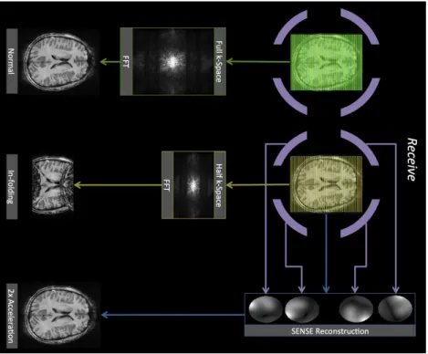
Figure 2.3: Schematic overview of 3 imaging strategies, each one indicated with arrows of a different color. Green: the standard reconstruction method (sum of squares) sampling the full k-space. Yellow: sum-of-squares reconstruction applied to a 2x under-sampled acquisition, resulting in an aliased image. Blue: parallel imaging (SENSE), using the receive sensitivities (purple) corresponding to the different coil-elements, applied to a 2x under-sampled acquisition.
Figure 2.4: Schematic overview of 3 transmission strategies, each one indicated with arrows of a different color. Green: the standard single-channel-tailored RF-excitation as described in section 1 of this chapter. Yellow: the effect of under-sampling k-space by a factor 2 during transmission. Purple: adopting parallel transmission, taking into account the transmit-sensitivity of each coil-element, to produce the same target magnetization while under-sampling k-space by a factor 2.