Boundary condition effects on vibrating cantilever beams

(1)

Boundary Condition Effects On Vibrating Cantilever Beams By

Jonathan David Monti Sc.B. Mechanical Engineering United States Naval Academy, 2012

Submitted to the Department of Mechanical Engineering in Partial Fulfillment of the Requirements for the Degree of

Master of Science in Mechanical Engineering at the

Massachusetts Institute of Technology September 2014

Signature of

Certified by

Author

Signature redacted

ent of Mechanical Engineering August 8, 2014

Signature redacted&

_.

_...

Martin L. Culpepper Professor of Mechanical Engineering Thesis Supervisor

Signature redacted

Accepted by... ... David E. Hardt Professor of Mechanical Engineering Graduate Officer

MAsSACHUSETTS WNTUTE

OF TECHNOLOGY

OCT 6

20]

(2)

(3)

Boundary Condition Effects On Vibrating Cantilever Beams By

Jonathan David Monti

Submitted to the Department of Mechanical Engineering on August 8, 2014 in Partial Fulfillment of the Requirements for the Degree of Master of Science in

Mechanical Engineering

ABSTRACT

Compliant mechanisms continue to see increased used in many areas of modem engineering. Their low cost, ease of production and manufacturing, and precision of motion have made them attractive solutions to many controlled motion systems such as nanopositioners or linear platforms. However, in some applications the stiffness requirements for the devices to function properly and the stiffness requirements for devices to survive outside effects such at vibration or impulse create a conflict which cannot be rectified with traditional engineering approaches. By utilizing boundary controls which acted only when a flexure reached a certain deflection, the original purpose of the device could be preserved while also reducing or eliminating the risk of failure from plastic deformation or brittle failure. By starting with the most basic of compliant mechanisms, the cantilever beam, and utilizing Buckingham Pi theory the dynamic behavior of the vibrating beams could be quantified and the associated variables used to tailor the design of a flexure and boundary control system. This research details the primary correlation between variables in a flexure system during natural frequency excitation and provides the mathematics necessary to implement boundary controls to prevent flexure failure. With this new information, cantilever style flexures can now be designed to operate in environments which previously would have put them at risk of catastrophic failure, and can allow for three to four times the increased range performance of a compliant mechanism in these environments without risk of failure. Furthermore, this research lays the foundation for the study of more complex flexures and multi degree-of-freedom systems.

Thesis Supervisor: Martin L. Culpepper

(4)

(5)

ACKNOWLEDGEMENTS

I would like to first and foremost thank the Lord for giving me the capacity, capability, and desire to pursue my various courses of study over the last seven years. Through him all things are possible, Philippians 4:13.

I would like to thank my mother and father, Steve and Suzanne Monti for the immeasurable amount of support they have given me throughout my life, and especially during the last seven years. I would like to thank my step mom, Liz Leoni-Monti, and my siblings, Steve, Chris, Karisa, Dante, and Giselle for the unique support each one provided. To my sister Christina I want to extend a special thank you for being my sidekick, best date, partner-in-crime, and energy drink delivery lady; LU SB ATRC. To my best friend Caleb, thank you.

I would like to thank the many professors and service men and women who I had the honor of spending four years by the Severn with. Professors Angela Moran, James D'Archangelo, and Ben Heineike deserve special thanks for the incredible amount of patience they displayed as my undergraduate instructors and for their dedication to my future and the futures of so many students before and after me. I would like to thank Captain MacDougall (USMC) who eight years showed humility and servant-leadership by dedicating time and energy outside his assigned duties to help a junior enlisted Marine start down an amazing path.

I would like to thank Professor Marty Culpepper for accepting me into his lab and mentoring me over the last few years; it has been a wonderful experience.

Lastly, I would like to thank Mr. Joe Scozzafava, Mr. Tom Macdonald, Mr. John Kuconis, and the Lincoln Lab team for their support, direction, and patience as I worked through this research. To the many unnamed people who supported me, helped me, listened to me gripe, or just let me sleep on their couch/floor/wherever after long nights of study, thank you!

(6)

FIGURES

Figure 1.1: Full System Diagram ... ₁₄

Figure 1.2: n5- 7i Correlation... ₁₄

Figure 1.3: LLCD System Graphic... ₁₅

Figure 1.4: Minotaur Payload Random Vibration During Flight ... 16

Figure 1.5: Large PAA N anopositioner... ₁₈

Figure 1.6: Large PAA Failure Points ... 19

Figure 1.7: Endless D esign Loop ... ₁₉

Figure 1.8: PCV N on-Linear M otion... ₂₁

Figure 1.9: A FM Variable Stiffness... ₂₁

Figure 2.1: Exam ple N anopositioners... ₂₃

Figure 2.2: Basic Com pliant Stage Diagram ... 24

Figure 2.3: Basic Stage FBD ... 24

Figure 2.4: Beam Geom etry Diagram ... ₂₅

Figure 2.5: Parallel (A), Serial (B), Hybrid (C) Flexure System s [18]... 26

Figure 2.6: Voice Coil Actuator... 26

Figure 2.7: Piezoelectric Actuator Types... 27

Figure 2.8: Piezo Geom etry Diagram ... 27

Figure 2.9: Contradicting Requirem ents... 29

Figure 2.10: Commercially Available Piezo Volumes, Deflections, and Force Outputs ... 30

Figure 2.11: Basic Cantilever Beam ... ₃₁

Figure 3.1: Stress in a Cantilever Beam ... ₃₃

Figure 3.2: Stress-Strain Curves... ₃₄

Figure 3.3: Com m on Com pliant M aterial Applications ... 35

Figure 3.4: Autom otive Strut A ssem bly ... ₃₆

Figure 3.5: Oil Dam per by ISOTECH ... ₃₆

Figure 3.6: Shock Excitations... ₃₇

(10)

Figure 3.8: Cantilever Beam Velocity Profile ... 40

Figure 3.9: Boundary Condition Styles ... 41

Figure 4.1: 4 Boundary Control Cases... 42

Figure 4.2: Superposition Method Illustration... 43

Figure 4.3: Cantilever Beam with Boundary Control... 43

Figure 4.4: Superposition Boundary Control Superposition Cases ... 44

Figure 4.5: Full Diagram of Cantilever Beam with Boundary Control ... 44

Figure 4.6: Cantilever Beam with Tip Mass... 47

Figure 4.7: Cantilever Beam with Tip Mass Exposed to Boundary Conditions... 48

Figure 4.8: W eighted Stiffness Zones... 49

Figure 4.9: Macro vs Micro Scale Stiffness... 50

Figure 4.10: Switch Bounce... 50

Figure 5.1: Complete System Diagram... 52

Figure 6.1: Linear Actuation Stage... 58

Figure 6.2: Stacked Piezo Performance ... 59

Figure 6.3: Phases of Linear Motion... 60

Figure 6.4: Linear Platform Dimensions ... 62

Figure 6.5: Physical Vibration Platform ... 63

Figure 6.6: Piezo Actuator Integration... 63

Figure 6.7: Piezo and Compliant Stage Assembly ... 64

Figure 6.8: Beam Test Sample Design ... 65

Figure 6.9: Physical Beam and Mass Test Samples ... 66

Figure 6.10: Boundary Control System ... 67

Figure 6.11: Line and Point Contact... 67

Figure 6.12: Boundary Control Induced Torque... 68

Figure 6.13: Test Setup Measurement Points ... 69

Figure 6.14: Physical Measurement Probe Setup ... 70

Figure 6.15: Platform Motion over Frequency Spectrum ... 71

Figure 8.1: System Variables and Pi Terms... 81

Figure 8.2: Higher Frequency Mode Locks...82

(11)

Figure 8.4: M etastable Region... 84

Figure 8.5: 5 vs 2 ... 85

Figure 8.6: Boundary Contact W aveform Types... 87

Figure 8.7:-E5 vs 6G ... ... 88

Figure 8.8: 5 vs 1... 89

Figure 8.9: Y vs Y offset... ₈₉

Figure 9.1: Practical Application Diagram...91

Figure 9.2: -7 Operating Line ... ... 92

Figure 9.3: Range of kc and 8G V alues ... 93

Figure 9.4: U seable k, and 6G Values... ₉₄

(12)

TABLES

Table 1.1: Nanopositioner Design Requirements ... 17

Table 1.2: Nanopositioner Performance ... 18

Table 5.1: System Variables ... 53

Table 5.2: Pi Term Formulation... 55

Table 6.1: Vibration Platform Specifications ... 58

Table 6.2: Measurement Point Variables... 69

Table 7.1: Static Cantilever Beam Properties ... 72

Table 7.2: Variable Mass Values ... 72

(13)

CHAPTER

1 INTRODUCTION

1.1 Introduction

The purpose of this research is to lay the foundation for implementing boundary control features in compliant mechanisms to prevent catastrophic failure due to vibrational forces. Current design methods do not include a tool to develop compliant mechanisms which will have boundary condition interaction over only a portion of their flexing range. The flexing range is defined as the range of motion which a mechanism can bend throughout without causing plastic deformation or catastrophic failure. This research focused on creating a way to predict the performance of a vibrating cantilever beam that contacts a boundary condition during its range of motion. This thesis seeks to create design guidelines for boundary conditions in compliant mechanisms, specifically cantilever beams, to allow them to maintain desired functions while mitigating survivability issues by introducing suitable boundary conditions. This will be accomplished by utilizing the Buckingham Pi method and a large set of test data. The implementation of boundary controls, which only interact with the mechanism when it reaches a point beyond its functional range, will allow designers to ensure a failure does not occur while preserving the desired static design performance. This research lays a foundation by analyzing a cantilever beam system exposed to vibration and provides a path for continued research into more complex compliant structures.

1.2 Background

1.2.1 Introduction to Final Product

Figure 1.1 is a basic graphic of the physical system and illustrates exactly how it functions as well as what the pertinent variables are in the test setup. A cantilever beam driven at

(14)

a frequency cOD, with _an _t

amplitude 6D, will cause the cantilever beam of length L

with mass m to bend and _6oWO

deflect, specifically _{at the} _L resonant frequency. If left

unchecked this motion would eventually cause the failure in the beam either through plastic deformation or complete failure in a brittle

material. Utilizing 6

D I

Buckingham Pi Theory and _{Figure 1.1: Full System Diagram} test data, we sought to determine what the exact effect of 6G, Lb, and La would be,

and how to utilize the variables in the system to prevent a catastrophic failure. Following the Pi term derivation we discovered one major correlation which led to the creation of an operating line between two Pi terms (Figure 1.2: 7r5- ni Correlation). This allowed variables

in a system to be properly adjusted to maintain original performance and also prevent the device from failing if exposed to random vibration.

If5 VS 1 8 6 - -- - - - -5j 0 ---- ------ 0 50 100 150 200 250 71

(15)

1.2.2 Specific Motivation for Research

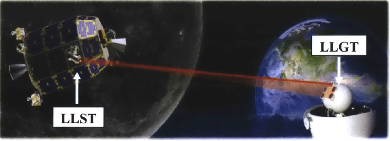
The Lunar Laser Communication Demonstration (LLCD) is a collaborative effort between NASA and MIT Lincoln Laboratory which sought to develop the first fully functional spaced based laser communications system [1]. The purpose of this project was to develop a communications system designed around lasers instead of the traditional RF technology. As designed the LLCD can transmit data at rates of up to 622 Mbps download and 20 Mbps upload. The system is comprised of two major components; the Lunar Lasercomm Space Terminal, and the Lunar Lasercomm Ground Terminal (Figure 1.3) [2].

LLGT

LLST

Figure 1.3: LLCD System Graphic

The Lunar Lasercomm Space Terminal (LLST) which sits aboard the LADEE spacecraft and has three sub modules; the optical module, modem module, and controller electronics module. The second component, the Lunar Lasercomm Ground Terminal (LLGT) consists of eight transreceivers and receiver telescopes and is built on a mobile platform allowing for deployment at various locations [2]. The nanopositioner, which motivated this research, is a subcomponent of the optical module on the LLST and is responsible for the Point-Ahead capability of the system by utilizing piezo-electric crystals on a compliant stage [3]. Due to relative motions of the LLST and the LLGT this nanopositioner must direct the outgoing beam with a Point-Ahead Angle (PAA). The greater the range of the PAA the greater the relative speed can be between the platforms while maintaining communications capabilities [4]. A greater PAA capability increases the overall capability of the platform by both increasing coverage area and

(16)

decreasing amount of LLST's required, or by allowing the same number of satellites to create redundancy coverage.

1.2.3 Current Technology

In order to increase the performance of each optical module, a PAA 4-6 times greater than the current capability was desired. This was not possible with the original nanopositioner due to its development around stacked piezo actuators. These actuators provide for high force outputs at the cost of total range (-kN blocking force, ~15gm free deflection, manufacturer dependent) [5]. Even using amplification arms, the stacked piezos would not be able to compensate for the limited deflection ranges they provided. The use of stacked piezos was motivated by the need for the nanopositioner to have a high natural frequency to avoid catastrophic failure during launch. The LADEE spacecraft is launched via the United States Air Force's Minotaur V rocket. Technical documents released by the U.S. Air Force indicate the random vibration frequency envelope and spectral energy density can reach range from 2-2000Hz and 0.002-.012g2/Hz respectively with 3.5344gRMS as seen in Figure 1.4 [6].

le-1

'ir

-le-2 C) a. 1e-31 ) 1 Oc 1000 Frequency (Hz) 100C 1@4025_069 Breakpoints Frequency PSD (Hz) (g2/Hz) 20 0.002 60 0.004 300 0.004 800 0.012 1000 0.012 2000 0.002 3.5344 gRMS 60 Sec Duration

(17)

The random vibration frequencies and spectral energy density mandate the nanopositioner platform must have a certain stiffness and natural frequency in order to survive the 60 second launch window, beyond which vibration is negligible (Figure 1.4). For this reason, stacked piezos with low range and high force output had previously been utilized, which greatly limits the PAA.

1.2.4 Large PAA Nanopositioner

In order to get the desired increase in PAA while abiding by the geometric constraints of the original system, stacked piezo actuators had to be replaced with bending piezo actuators. These bending piezos would allow for PAA's 4-6 times higher than the current solution, at the cost of overall stiffness. Table 1.1 lists the requirements and constraints put forth for new the nanopositioner design.

Table 1.1: Nanopositioner Design Requirements

Nanopositioner Property Required Units

Translation X +1- 50 m Translation Y +1- 50 gm Length (Z) <22.8 mm Width (X) <20 mm Height (Y) <17 mm Natural Frequency >1000 Hz

Drive Voltage -50-200 Volts

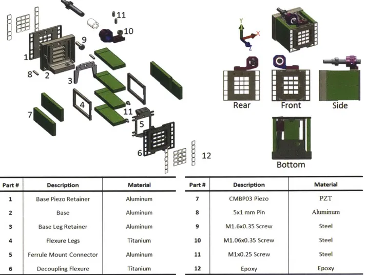
With these design requirements in mind the nanopositioner in Figure 1.5 was designed utilizing CMBPO3 Bending Piezo Actuators manufactured by Noliac. These bending piezos are capable of +/-85pm free deflections and have a blocking force of 5.5N [6], which was the largest range and blocking force available from an off-the-shelf plate bender with suitable geometry. With these piezos at the heart of the design, the nanopositioner was capable of meeting or exceeding all design requirements from Table 1.1 as can be seen in Table 1.2.

(18)

1Q 1

L

Y Rear Front 12

Part # Description Material

1 Base Piezo Retainer Aluminum

2 Base Aluminum

3 Base Leg Retainer Aluminum 4 Flexure Legs Titanium

5 Ferrule Mount Connector Aluminum

6 Decoupling Flexure Titanium

slwe

Bottom

Part # Description Material

7 CMBPO3 Piezo PZT

8 5x1 mm Pin Aluminum

9 M1.6x0.35 Screw Steel

10 M1.06xO.35 Screw Steel

11 M1xO.25 Screw Steel

12 Epoxy Epoxy

Figure 1.5: Large PAA Nanopositioner

Table 1.2: Nanopositioner Performance

Nanopositioner Property As Designed Units

Translation X +/- 57 gm Translation Y +/- 58 pm Length (Z) <21.7 mm Width (X) <20 mm Height (Y) <17 mm Natural Frequency 2095 Hz

Drive Voltage 0-200 Volts

87

P1

b

1

(19)

Although the large PAA nanopositioner meets or exceeds all desired properties, vibration platform testing must still be performed to ensure survivability in a launch scenario. Early FEA indicates the platform has a factor of safety just over 1, with failure occurring at the

base of the piezos in the corners as indicated in Figure

Failure Points

1.6. With a factor of safety just over 1 and any failure in

these piezos causing not only a major performance setback within the system but even larger problems due

to fragmented piezo material free floating throughout the Figure 1.6: Large PAA Failure Points

optic system, a more robust and effective survivability setup was preferred. This was the fundemental motive which drove the research conducted in this thesis.

1.3 The Endless Design Loop

Failure7 Occurs Need to Make Desig Less Space Limited By Larger Constraint DReg esiLo

Design

LooF

Needed Stiffness Below Failure Need Stiffer Mechanis Ne edGreater Force/Range Output From Actuators Need More Space

Force/Range output

Figure 1.7: Endless Design Loop

The primary

problem with current philosophy, especially in regards this area of design, is that if the stiffness needed for functionality is considerably lower than the stiffness needed for survivability it creates an endless loop (see Figure 1.7).

There are ways to break out of this loop; use higher force actuators, higher strength materials, etc. However, these break

(20)

point items are highly researched and movement is now incremental. It is unlikely that next year a company will introduce a piezo with all the same dimensions and characteristics of current ones only with double the force output. Same goes for the materials used in construction.

1.4 The Larger Picture

Although the motive behind this research was a specific application, increased survivability during rocket launch, the research has applications beyond this single area. Intelligently designed boundary control could be used not only for catastrophic failure mitigation, but stiffness zone designing, and controlled stiffness increases (to be discussed in further detail later). In the specific satellite situation discussed, proper implementation of the boundary condition controls could result in a satellite network performing anywhere from 4 to 6 times more effectively than currently designed. This means the total network cost for a full coverage satellite network could be reduced by 4 to 6 times, or there could multiple layers of redundancy in a lasercomm network. With a single Minotaur series rocket costing $50 million to procure and launch (each Minotaur rocket can carry up to seven satellites) [8], and the average cost of a satellite at nearly $100 million [9], the cost savings to this program alone could be in the billions (initial LLCD launch was lunar based, still yet to be determined how orbital satellite network would be arranged or how many of the current generation of LLST's would be required). This is the larger impact cost. In a more direct sense, the previous nanopositioner was in development for nearly half a decade by a team of engineers at Lincoln Lab. Boundary control research will give designers a clearer understanding of compliant mechanism design subjected to random vibrations.

Compliant mechanisms have become increasingly popular, especially in the area of precision control. As stated previously, compliant mechanisms are the choice platform for long range communications laser positioning. However, the larger application of compliant mechanisms includes surgical tools [10], precision machining [11], and automotive and aerospace applications [12], to name a few. Compliant mechanism are growing in popularity largely due to their reduction in production cost (many are designed and built as single piece structures without the need for assembly or multiple stages of production) and increase in performance due to the single unit design. The performance benefits come from reduced size

(21)

and weight, reduced wear [12], and little or no assembly means no friction, or error due to imprecise parts fit/alignment. All compliant mechanisms are built with a balance between overall stiffness needed for the device application, and stiffness required to ensure part reliability and survivability. This research seeks to give compliant mechanism designers a new tool to apply to a design which will preserve the stiffness required for application, while addressing the stiffness required to ensure reliability and survivability.

1.5 Prior Art

Very little work has been done previously in this area of research. Nearly all work containing similarities has to do with AFM or PCV research. The closest research content to what is contained in this thesis was conducted by Clemens T. Mueller-Falcke and has to do with variable stiffness in AFM cantilever beams (Figure

1.9 [13]). His research focused on utilizing external Figure 1.9: AFM Variable Stiffness

beams which would be electrostatically charged causing them to bond to the original beam, thus changing the stiffness of the beam. This research does directly apply to the issues being discussed in this thesis since the adjustments were made deliberately and at determined times and was used as an active system. Upon activation the system would merely take on a set new stiffness value, but still move and function as a cantilever beam (essentially the same as changing the geometry). This process would not apply to case being address in this since a passive step-function stiffness increase is required at a predetermined deflection. The other major research into this field was conducted by David Freeman. He characterized deflection in Pressure Control

F F Valves contacting an external

boundary, but his research deals with valve plates with large

Figure 1.8: PCV Non-Linear Motion deformations into the non-linear region of motion, and that research is only concerned with static deformations (Figure 1.8 [14]). In most engineering practices, designing a deflecting part such that it will contact another body and continue deflecting would generally be avoided due to the friction, contact stress, shock etc. This could explain the limited amount of research in this area.

(22)

1.6 Preview of Thesis Contents

This thesis will:

* Lay the foundation for the research

o Introduce the fundamentals of flexure design

o Introduce the basic concept of boundary condition control fundamentals of boundary condition control and explain current boundary condition control styles

o Discuss the benefits of boundary condition control

" Discuss the math behind the proposed boundary condition controls o Basic beam bending math

o Static beam bending with contact on a rigid body o Beam dynamics and math limitations

" Introduce Buckingham Pi method " Discuss vibrating beam test theory

o Scope o Assumptions

" Detail vibrating beam test setup o Vibration test bench design

o Beam sample design and test fixture design o Test theory assumptions

" Discuss test process and data handling " Analyze Buckingham Pi associations " Complete a practical application example " Introduce future work

(23)

CHAPTER

2 Fundamentals of Flexure Design and Motivation for Specific Research

2.1 Compliant Systems Nanopositioner Design

2.1.1 Compliant Stage

Most compliant mechanism based positioner designs consist of a compliant stage and an actuator. The compliant stage is then broken up into 3 distinct zones; ground, flexures, and stage (Figure 2.2). Figure 2.1 shows three examples of modem piezo driven nanopositioners (for intellectual property reasons, exact design schematics not available); 1. nPXY60-258 by nPoint Inc. [13], 2. P-612.2 Compact XY Positioner by Physik Instrumente [16], 3. PZ 250 CAP WL by Piezosystems Jena [17] .Indicated in the figure are the ground portions (solid black line) and actuated stage portions (dotted line) of each positioner, with the piezo and exact flexure system being enclosed within the shell of the device.

Figure 2.1: Example Nanopositioners

Ground indicates the portion of the device which is considered to be stationary, often locked or screwed to a bench or larger machine. The flexures are responsible for allowing, restricting, or directing the motion of the stage. The stage is where the object to be manipulated

(24)

would be secured, and the actuator (in the above cases a piezo), is responsible for supplying the force to move the stage into place. Figure 2.2 is a simplified diagram of what this would look like in a basic cantilever compliant mechanism.

TFoi~e

\ N \ \~' >~ N \ ~> N

7

Figure 2.2: Basic Compliant Stage Diagram

The force and deflection values are mathematically tied together. In order to increase the stage deflection the force must be increased, assuming the max deflection of the actuator has not been reached, or the flexure stiffness must be decreased. In the case of the compliant stage in Figure 2.2 the governing mathematics are fairly

basic and straightforward. If the compliant stage

_{X +}

above is simplified into a single degree of )

freedom system, as can be seen in the free body diagram in Figure 2.3, and the deflections are

large enough that internal stresses can be ignored

Act

(simplified beam equations instead of

Timoshenko beam equations), then relating the

actuator force (FAct) with the static deflection

F

requires it to be balanced with the spring force

exerted by the flexure (Fsp,). _{Figure 2.3: Basic Stage FBD}

FAct = Fspr

I

bty

(25)

And

Fspr = Ksprx

with x being the magnitude of deflection in the stage, then

FAct = Ksprx

The stiffness Kspr has previously been determined to be

Kspr =

3EI/L

3 _and

_I

₌

_bh

3

_/12

with E, and L being the modulus of elasticity of the specific material used and the length of the beam respectively. I is the moment of inertia for the beam and consists of the beam dimensions both in line with the direction of motion, h, and perpendicular to the motion and the length, b, Figure 2.4.

lhirectio

01 *0 X

b

Figure 2.4: Beam Geometry Diagram

Therefore, the governing equation which relates the force output of the actuator to the stage's deflection in the X direction is

(26)

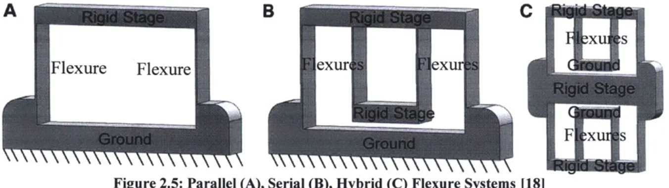
This is one of the most basic forms of a compliant mechanic being used as a positioning stage, and as such the mathematics are fairly straightforward as well. There are many more configurations of flexures that can be used to direct actuator motion in a specific axis. Figure 2.5 [16] shows three examples of flexure systems without an actuator, each with increasing complexity, and each with a different purpose.

C

Figure 2.5: Parallel (A), Serial (B), Hybrid (C) Flexure Systems [181

There is much literature detailing how to develop flexure systems, the math which governs specific configurations, and the expected performance and capability that can achieved with various flexure structures. These more complex systems will not be discussed in this thesis unless pertinent to the content of the chapter.

2.1.2 Nanopositioner Actuation Solutions

Although the design of most positioning stages is fairly straightforward, problems begin to arise when the requirements for a stage become contradictory. This is the case in the previously discussed Large PAA nanopositioner. Due the size constraints on the device, piezoelectric and voice coil actuators (Figure 2.6 [20]) are the only two widely available actuators which are suitable for this application. For voice coils the governing equations are

Figure 2.6: Voice Coil Actuator

F

=

kBLIN

Where F =force, k-constant, B=magnetic flux density, I=current, L=length of conductor, and N=number of conductors [19]. All things being constant this means that the force output on a

(27)

voice coil is directly proportional to the length of the conductor. Therefore, as the package size decreases the force output of the voice coil decreases as well, this causes a problem when designing for space-limited applications.

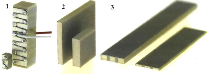
The second primary actuator used is the piezoelectric actuator. These break into many different types; stacked (1), plate (2), and bender (3), to name a few (Figure 2.7).

2

3

Figure 2.7: Piezoelectric Actuator Types

For piezoelectric actuators the general force equation for zero deflection (blocked force) is

Fmax

= kTALO

where k1=piezo actuator stiffness, and ALo=max displacement without external restraint [21], and

kT-axial =

AEIL

kT-transverse =

3EI/L

3 and Force Output A Force Output

A =

wt

I

=

bh

3

/12

where E=modulus of elasticity for the specific material, and L, w, t, b, and h are illustrated

in Figure 2.8. Ground

Axial Actuator

NGround Transverse Actuator

(28)

Once again, as was the case with the voice coils, as the package size decreases the output force also decreases (depending on which element of the geometry is being reduced).This is without even taking into account the specifications for needed stroke length.

With the two primary actuation methods being governed by physics which limit force output based upon package size, designers are forced to develop a stage which can achieve the desired performance while staying at or below the force output threshold for the specific actuator chosen.

2.2 _{Contradicting Requirements for Compliant Stages in}

Harsh Environments

For many nanopositioner applications the environment will be well controlled with respect to vibration and in some cases will have unique requirements demanded of the device. The requirements may include waterproofing, electrical shielding, thermal insulating, or any one of a number of other requirements. For the most part these requirements can be met by a skilled engineer developing an intelligent design. Most requirements are ancillary and can be designed within or around the original device. In some instances the original device may need to be modified. However, none of these requirements are such that they must absolutely interfere with the device's operation to complete their purpose. In rare cases, these nanopositioners will be put into environments where there will be high levels of random vibration. In order for these positioners to survive the harsh environments they must be capable of withstanding the vibrational forces exerted on them. This is the where the contradiction arises.

In order to keep an object from failing in a high vibration environment, the designer has two options; make it more compliant, or make it stiffer. In the first case, make it more compliant, the designer assumes that the deflection in the device is such that rather than trying to fight it, it is wiser to allow the device to move freely. The designer can adjust the design of the device such that the maximum deflection felt by the positioner is less than the deflection required to reach the maximum allowable stress in any area of the device. The problem with

(29)

option is that most compliant stages require actuators which are fairly rigid, and the option to simply make them more compliant does not exist. For instance, if a designer chooses to modify the geometry of a bending piezo actuator he or she does so at the cost of performance (either free stroke or blocked force). In the second case, the designer can choose to increase the stiffness of the device. This is most easily done by adjusting the geometries of the flexure elements, or

changing the material used in the positioner. However, changing the material is unlikely since the original material was chosen for its specific properties, likely its low modulus of elasticity and high yield stress. That leaves the designers one viable option; adjust the geometry of the flexures to make it stiffer.

In many cases in order to ensure the device will survive the vibration environment the designer must ensure the natural frequency of the device is above the range of vibration frequencies it will be exposed to. Any time a device is exposed to a vibrating frequency equal to its natural frequency the energy in the device builds and will manifest itself as large deformations within the device. Natural frequency is governed by the equation

fn = Ik/M (radians) or A

k/r

(Hertz)

21r

Wheref,=natural frequency (radians/hertz respectively), k=equivalent stiffness, and m=tip mass.

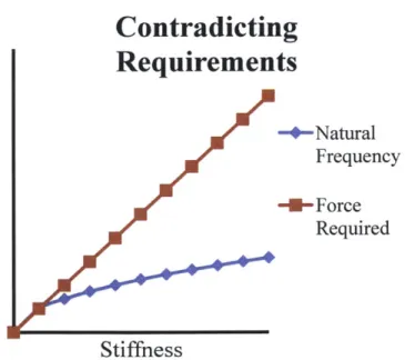
Stiffness must be increased or tip mass decreased in order to raise the natural frequency. This works assuming the designer can then adjust the actuation device to cope with the new stiffness values. In some cases this may not be possible due to power, geometry, cost, or a number of other limiting factors. If the designer is unable to adjust the actuation device, he or she is at an impasse. Figure 2.9 shows how the contradiction manifests itself in regards to stiffness, force required (to maintain the same max

Contradicting

Requirements

-4-Natural Frequency -U-Force Required Stiffness

Figure 2.9: Contradicting Requirements

(30)

deflection), and natural frequency (assuming tip mass is constant) in a basic cantilever beam. The contradiction is the same in other more complex compliant mechanisms as well since fundamentally natural frequency is tied to stiffness and stiffness dictates force required. As can be seen in Figure 2.9, as stiffness increases the force required increases linearly and proportionally, however, natural frequency increases by the square root of the increase in stiffness. What this means for the designer is that any attempt to increase the natural frequency brings with it a severe increase in the force required. As previously discussed in Section 2.1.2 any increase in force required brings with it the mandate that the geometric size of the actuator must also be increased. For instance, if the designer attempts to raise the natural frequency of a device by a factor of 2, the force required increases by factor of 4, and the resulting changes in volume and deflection of commercially available piezos to meet this force requirement are

illustrated in Figure 2.10 [22][23] [24].

Blocked Force vs Volume Blocked Force vs FreeDeflection

1000 3000 C" 80 0 * E 2500 E 2000 E 600 .50 m a BA -1500 4' 400 jl 2 * .1000 . ... 20B 500... .. 0 0 B 0 2 Force (N) 4 6 0 2 Force (N) 4 6

Figure 2.10: Commercially Available'Piezo Volumes, Deflections, and Force Outputs

In case A, if the designer needs to double the blocked force and maintain a free deflection of ~500pm for the positioner to work properly then the volume of the piezo increases from 156mm3 to 450mm3. Even more significant is that due to the nature of piezoelectrics the volumetric increase will likely be the result of a large change in one aspect of the geometry rather than a proportional increase in all geometries. For case A the length and width remained relatively constant (max change of <20%), but the thickness increased nearly threefold from 0.65mm to 1.8mm. Conversely, in case B if the designer needs to maintain the piezo's volume while increasing the output force from 1.2N to 4N the loss to free deflection is nearly 60%, dropping from 390gm to 160gm. These two examples illustrate the fact that if the designer has to

(31)

decrease the vibrational sensitivity of a positioning stage in a space-limited application they are left with an impossible situation (see Figure 1.7: Endless Design Loop).

2.3 Finding a Mechanism to Interrupt the Endless Cycle

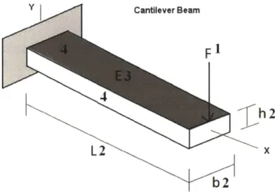
In order to break the endless design loop, we need to look at every unique element in the design phase and determine which one may still be manipulated. Figure 2.11 shows the basic cantilever beam with all major properties listed (ones that directly impact the problem needing to be addressed). Cantilever Beam

F'

4 h 2 L 2 x

b2

Figure 2.11: Basic Cantilever Beam

As previously discussed, (F, 1) force is fixed or limited due to geometric constraints, the size of the beam (L, b, h (2)) is limited by both geometric constraints as well as stiffness limitations from the force output of the actuator, (E, 3) modulus of elasticity has likely already been determined based on stage application and is also constrained by force limitations. This leaves no viable option within the system to effect change. However, one area we haven't considered is the surface areas of the flexure (4). In most flexures this surface is a smooth, flat surface, making it ideal for interaction with another body in order to limit its overall deflection. Having this surface area interact with another body at some point beyond its normal flexing range will cause a change in stiffness which can be used to prevent plastic deformation or catastrophic failure.

(32)

2.4 The Idea of Boundary Control

By using a boundary control mechanism which does not contact the stage during normal operation the stiffness of the device can be changed without interfering with its standard functions. A boundary control could be any body that interacts with the deflecting portions of the stage in such a way as to alter the behavior of the system. Generally speaking, it is unwise to have rigid bodies contacting in a compliant stage. This interaction leads to friction, contact stresses, and shock loading. None of these are desirable characteristics in a compliant stage, and should generally be avoided. But if a boundary control can be implemented in such a way as to prevent ultimate failure of the stage, then the tradeoff to a designer is worthwhile.

(33)

CHAPTER

3 Boundary Condition Fundamentals

3.1 Previous Boundary Condition Use

3.1.1 Nonuse

The nonuse of a boundary condition in the applications discussed would result in a failure of the flexures or actuators either by plastic deformation, buckling, or brittle failure. When talking about the flexures themselves, plastic deformation will be the likely manner in which a beam fails. In regards to a piezo actuator, brittle failure is likely to occur due to its material properties.

Due to the design nature of the flexures in a compliant stage plastic deformation will occur at the very base first (Figure 3.1). The equation for the stress in a deflecting beam is

Mc bh3 P

=

- and I ..

1 12

where u'=stress, M=moment at specific point, c=distance from neutral axis, I=area moment of

inertia, (I defined in 2.1.1). For a uniform geometry C cantilever beam the max stress is found in the very

base of the beam, this is where the moment is L highest. The equation to determine the max stress

from the beam in Figure 3.1 is

PLc

(34)

Looking at the stress-strain curves for

two commonly used flexure and actuator - -

--materials (aluminum and PZT) (Figure 3.2)

[25] [27], we see that the yield stress for a UyAL...'275 Mpa

generic piezoceramic is far lower than the

- -6061-T6

yield stress for a flexure. This makes the -Piezoceramic

bending piezo stress the point which must be design around. Without any boundary

condition interaction a compliant mechanism Uypzr ....'5 Mpa subject to a vibration force with enough

energy will cause fracturing at the base of the Figure 3.2: _{Figre .2:Stress-Strain Curves}E

bending piezo. The assumption of this

research is that the vibrational forces the positioning stage will be subject to will cause the max stress in the base of the piezo actuator to be greater than the established yield stress for the specific piezo material used.

3.1.2 Soft Stops

A soft stop is probably the most commonly used means to prevent a bending element from reaching its yield stress. By inserting a material with a low stiffness the deflecting beam has some interaction with the soft stop which absorbs energy and limits the overall motion the beam can be subjected to. Soft stops can be broken down into two major categories; compliant materials and damping.

3.1.2.1 Compliant Material

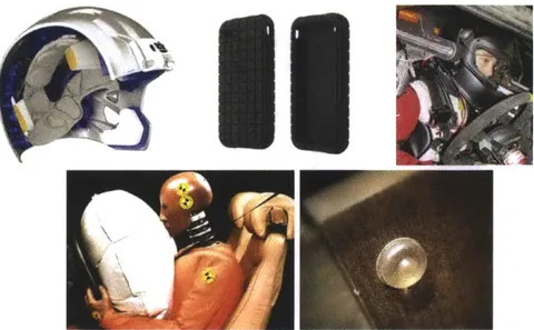
A compliant material is any material which has a specifically selected stiffness such that when an object interacts with it there is a period where the compliant material exerts a reactive force to prevent the further motion of the original object. Compliant materials are also used to reduce the shock loading felt by a deflecting object or any object in motion. This concept is used in many every day applications. Common applications include airbags, race car head restraints,

(35)

football helmets, rubber stops on cabinets, and protective cell phone cases (Figure 3.3) [27][28][29][30][3 1].

Figure 3.3: Common Compliant Material Applications

The major issue with using compliant materials (rubbers, plastics, etc.) is the outgassing that occurs throughout the object's lifetime. Outgassing is the release of internally held gasses in rubbers, polycarbonates, and many other synthetic materials [32]. The effects of outgassing are amplified in the research specific case by the vacuum present in the space bound platforms. In sealed or controlled applications this outgassing can introduce particles to the atmosphere which are harmful to the overall performance of the system.

3.1.2.2 Damping

Unlike soft stops, which act upon an object with as set reactive force consistent with its stiffness properties, damping is the process which resists motion based upon its velocity at a given time. For instance water can be used a damping mechanism. If a person were to slip their hand into water slowly palm down, the hand would easily cut through the water and sink. However, if a person were to slap their hand against the water with a high velocity the water would exert a reactionary force on the hand to slow its speed; this is damping. A common example of a damping is the strut assembly in a motor vehicle. The strut assembly is comprised

(36)

of two major parts (Figure 3.4). First is the coil spring which acts as a compliant material and deforms when a load is placed on it. The problem with having only a coil spring is that when a vehicle hits a bump the force exerted on the spring is greater than the force which the spring can sustain. This is where the damping system begins to act. The shock absorber is the internal tube portion of the strut

ce Wg and acts to resist fast motions, like those induced when

hitting a pothole. In general, damping is the preferred sUa method of reducing and limiting the effects of shock on a

svrw r.osystem. Because the natural frequencies of most systems Sreti rRack Sk are relatively high (above single digit frequencies) the

velocity of the oscillating mass is also high. This property makes it an ideal setup to introduce damping. However,

Tie the issue with damping is that most damping materials and

systems include a Figure 3.4: Automotive Strut Assembly viscous element (Figure 3.5) [33]. This means they require a housing mechanism or some way to control the damping substance. Since the designer is already working in a space limited capacity this poses a geometric problem. Also, because of the viscous nature of the damping substance, long term use and containment of the substance brings with it a whole new set of design complications.

Figure 3.5: Oil Damper by ISOTECH

3.1.3 Hard Stop

Another commonly used method of preventing a bending element from reaching its yield stress is a basic hard stop. This is a solid material stop which essentially takes the beam element's stiffness to infinity upon contact. If a person opens a self-closing door at a business, this door has some stiffness associated with its operation. If the person continues to open the door until the handle on the other side smacks into a wall, this would be considered a hard stop. The problem with utilizing a hard stop is that it induces shock loading in the system. If a door is

(37)

slammed open into a wall, the door will begin the visibly vibrate after bouncing violently off the wall. Similarly, a deflecting stage will collide with a hard stop and induce further vibration and shock loading from the contact. Shock load is the common term for the force applied to an object which causes sudden acceleration or deceleration. A common way of analyzing the shock imparted on a system is the velocity change method. The shock transmitted when one rigid body collides with another is governs by the equation

_ V(27rfn)

Typical ShoCK Excitations

and the deflection caused by the shock is

A

d =V

27rfn _t

where G,-transmitted shock, V=velocity V

and is derived from Figure 3.6 [35] (specified for gravitationally controlled systems, can be modified for other

accelerating forces), g=acceleration due to V V2 gravity (or any acceleration inducing Vem mechanism), andf,=natural frequency of

the system.

F

Shock loading is influenced by three factors; mass of the system, the

speed of the system just prior to impact, X

and the rate of change of the acceleration

in the system [36]. The rate of change of =

the accelerations is related to the stopping Trm.oAst4

distance of the system as seen by the basic motion equation

NOt _d(t) ecto d(t)dt v t V2 ---V1 -V V =V2gh(inekastic impact) V 2 V2gh (elesic mpact) Shock Free-Fa Impact

igure 3.6: Shock Excitations

..ration Rcta4.a. A.a.on

:04on Vnwd4n Accewbon

AV = V

0

+ at

Where A V=change in object velocity, V=velocity of the system prior to impact, a=acceleration, t=time

(38)

To see a practical example of the forces induced in shock loading Figure 3.7 illustrates a 0.001kg aluminum ball on a negligible stiffness cantilever beam with 0.001m radius about to contact a grounded aluminum plate at 1m/s. To determine the stopping distance we need to know how far the ball travels following its initial contact with the wall. To get a general idea of this distance, we will use the equation for Hertzian contact deformation [37]

E=70Gpa Vo=lm/s -- *

Figure 3.7: Shock Loading Example

6 1 2F

2(Re 2Ee)

and

Re 1 1 1

R₁ R₂

where 6=deformed deflection, Re=equivalent radius, R₁₂=radii of object 1 and 2 respectively, F=force of ball in motion, Ee=equivalent modulus of elasticity.

Combining the Hertzian contact equation with the basic displacement equation

x =

Vt+ at2

2 (11)

where x=center displaced distance of the ball (deflection), V=velocity upon impact, a=acceleration, t=time for ball to reach a zero velocity, results in the equation

1 2

Vt+1 a

2 1 (1 -3 3F -3

V

2t+-at

=

02 \JRek 2Ee) (III)

Using Newton's second law we can replace force with mass and acceleration, and we know that acceleration is merely the rate of change of velocity

F

=

ma (IV) and dv dv __)

a (V) this case s

(39)

substituting (IV) and (V) into (III) results in 2 1/ d\

-V

1ldv 2 1 3 3m-VOt + )- (VI) 2 (=dt2) Re 2Ee

leaving t as the single unknown variable.

Using all the givens from the original problem:

Variable Value Units

V 1 m/s

Vf 0 m/s

Re 0.001 m

m 0.001 kg

Ee 7x1010 N/m2

we find that t=0.0136ms, which can use to calculate the acceleration of the object using

AV = at

And we know A V=-lm/s, and t=13.6ns, thus a=-73000m/s2 _{which can be plugged back into}

equation (IV) to solve for F=73N imparted on the ball during the collision. As a comparison this same ball sitting in the palm of your hand would only exert a force of 9.8mN, and the same collision at a one third reduction in velocity would reduce F to 48N. Furthermore, if the At value could be increased by a third, the force imparted could be reduced by one third as well. Because a pure contact has such small At it is not unreasonable to assume that it could be increased by a factor of 100 or more with a boundary contact which would allow motion to occur at a higher stiffness value beyond contact. These types of forces and loads should be avoided whenever possible, especially in compliant stages using piezo actuators due to the brittle nature of piezoceramic materials. For a further look at contact pressures and stresses see "Precision Machine Design" by Alexander Slocum [37].

In most cases a hard stop is used at the point of highest deflection. In the case of a cantilever beam, this would be the free end of the beam. The problem with this application is that the free end of a cantilever beam is also the point of highest velocity. Since the maximum

(40)

Free End deflection of any point on a cantilever beam is

100 - - 100 _{proportional to the velocity at that same point, it would}

90- - 72.9 _{follow that the further you get from the base of the beam}

80- - 51.2 _{the higher the velocity at that point. Since deflection is a} 70- - 34.3 _{properly of the length of the beam cubed, the velocity at}

60- -- 21.6

% Beam % Tip a given point on the beam increases by that factor as

Length 50- - 12.5 Velocity _{well. Figure 3.8 illustrates the velocity of a beam at}

40- - 6.4

various points as a percent of max tip velocity. If the

30 - - 2.7

20-- -. 8 hard stop were to be moved one third the way down the

10- - 0.1 beam, the induced shock would be reduced by over

-_ 70%. Furthermore, if the hard stop is moved down the

beam towards the fixed end, there will be a mass above

Fixed Base

Figure 3.8: Cantilever Beam Velocity Profile _{the hard stop which will continue its motion after}

contact has occurred with the hard stop. This means that stopping time is greatly reduced, thus reducing the force exerted on the beam from the hard stop.

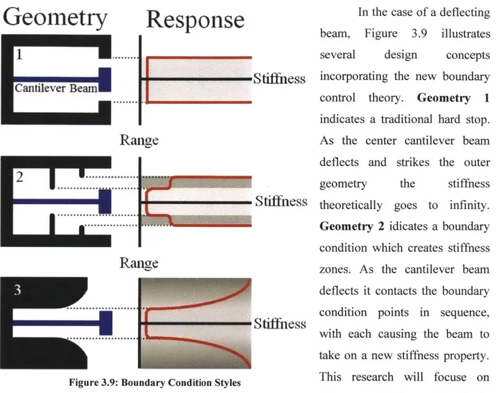
3.1.4 Boundary Condition Control: The Space Between Hard Stop and No Stop As was discussed in the previous sections, if a designer is at a point where a compliant mechanism will fail due to vibrational forces a "no stop" is not an option. Conversely, a hard stop would impart extremely high forces on to the deflecting stage. However, if a hard stop is moved away from the point of maximum deflection on a beam or stage, this greatly reduces the shock loading as well as increasing the stiffness of the device thus resisting further motion. We will call this implementation of a hard stop a boundary control, and illuminate the effects and proper use of this new concept.

(41)

Geometry

Response

In the case of a deflecting beam, Figure 3.9 illustrates

1

... several design concepts

Stiffness

incorporating the new boundary

Cantilever Beam control theory. Geometry I

indicates a traditional hard stop.

Range

As the center cantilever beam deflects and strikes the outer

... ... geometry the stiffness

Stiffness

_{theoretically goes to infinity.}

... _{Geometry 2 idicates a boundary}

condition which creates stiffness

Range

_{zones. As the cantilever beam}

deflects it contacts the boundary

... _{condition points in sequence,}

... with each causing the beam to

take on a new stiffness property.

Figure 3.9: Boundary Condition Styles This research will focuse on

Geometry 2 using only a single stiffness zone change. Geometry 3 is a rolling boundary condition in which beam stiffness is directly related to its exact deformed position at any time after contact. Using Geometries 2 and 3, a designer could not only prevent a catastrophic failure, but design in specific stiffness zones.

(42)

CHAPTER

4 Boundary Condition Math

4.1 Static Behavior

4.1.1 4 Static Cases

We must analyze 4

different cases In order to 1. Standard Cantilever CF

X CaseO explore the mathematics behind

the static operation of a boundary

1. Effect of varying contact point in "X" control. Figure 4.1 illustrates the1

four cases which when analyzed j

-make up the full extent of static 2. Effect of varying contact point in "Y" Case 2 boundary control mathematics.

For the content in this thesis, all

3. Effect of slope boundary condition

external forces are treated as Case 3

purely perpendicular. _{Case 0}

indicates a standard cantilever Figure 4.1: 4 Boundary Control Cases

beam with linear deflection. Case 1 occurs when the deflecting beam in Case 0 is combined with a support at some point along the length of the beam. Case 2 is a support that is not initially in contact with the deflecting beam; as such its mathematical equivalent is a combination of Case 0 (prior to contact) and Case 1 (after contact). Case 3 is a combination of all three with the X-Y contact point being a product of the total tip deflection, for this research we will not address this style of boundary condition and will instead focus primarily on Case 2.

Boundary condition effects on vibrating cantilever beams

Signature redacted

Signature redacted&

.

...

Signature redacted

OCT 6

20]

ABSTRACT

ACKNOWLEDGEMENTS

CONTENTS

FIGURES

TABLES

CHAPTER

1

INTRODUCTION

1.1 Introduction

1.2 Background

LLGT

LLST

1.2.3 Current Technology

'ir

1.2.4 Large PAA Nanopositioner

L

1

Failure Points

1.3 The Endless Design Loop

Design

LooF

1.4 The Larger Picture

1.5 Prior Art

1.6 Preview of Thesis Contents

CHAPTER

2

Fundamentals of Flexure Design and Motivation for Specific Research

2.1 Compliant Systems Nanopositioner Design

2.1.1 Compliant Stage

TFoi~e

7

X +

Act

F

I

Kspr =

3EI/L

I

bh

/12

lhirectio

b

C

2.1.2 Nanopositioner Actuation Solutions

F

=

kBLIN

2

3

Fmax

= kTALO

AEIL

3EI/L

A =

wt

I

=

bh

/12

2.2

Contradicting Requirements for Compliant Stages in

Harsh Environments

k/r

Contradicting

Requirements

2.3 Finding a Mechanism to Interrupt the Endless Cycle

F'

b2

2.4 The Idea of Boundary Control

CHAPTER

3

Boundary Condition Fundamentals

_.

_...

_{X +}

_I

_bh

_/12

_{Contradicting Requirements for Compliant Stages in}