An analysis of quadrotor flight in the urban canopy layer

An Analysis of Quadrotor Flight in the Urban

Canopy Layer

by

John Ware

Submitted to the Department of Aeronautics and Astronautics

in partial fulfillment of the requirements for the degree of

Master of Science in Aeronautics and Astronautics

at the

MASSACHUSETTS INSTITUTE OF TECHNOLOGY

June 2016 'Se

\>er 2.o\ 3

Massachusetts Institute of Technology 2016. All rights reserved.

//

/

Signature redacted

A uthor

...

...

Iepartment of Aeronautics and Astronautics

May 19, 2016

Signature redacted

C ertified by

...

...

...

-I

Nicholas Roy

Associate Professor

Thesis Supervisor

Signature redacted

Paulo C. Lozano

M S INSTTUTE

Chair, Graduate Program Committee

T HNOLOGY.

An Analysis of Quadrotor Flight in the Urban Canopy Layer

by

John Ware

Submitted to the Department of Aeronautics and Astronautics on May 19, 2016, in partial fulfillment of the

requirements for the degree of

Master of Science in Aeronautics and Astronautics

Abstract

This thesis presents two distinct bodies of work concerning quadrotor flight in urban wind fields. The first attempts to characterize a quadrotor's ability to exploit urban wind fields for improved flight performance. A computational fluid dynamics model is used to obtain a wind field estimate given a 3D model of the environment and a prevailing wind estimate. Minimum-energy trajectories are then found through the environment using an empirically derived power consumption model for a specific quadrotor platform. It is shown in simulation that a minimum-energy planner aware of the wind field outperforms a naive, wind-unaware planner over metrics such as total energy consumption, time to goal, and failure rate. The second component of the work focuses on the development of an onboard wind sensor for quadrotors. Although it is not yet clear how to integrate these measurements into a global wind field estimate or use them in a planner, it is intuitive that on-board measurements could inform the local wind field estimate or validate the global one. Accordingly, an effort was made to integrate an existing microelectromechanical flow sensor into a quadrotor platform. Initial results from full-scale tests in the Wright Brothers wind tunnel at MIT demonstrate the the sensor's performance in flight and hover conditions.

Thesis Supervisor: Nicholas Roy Title: Associate Professor

4

Acknowledgments

Thanks to my wife and family for supporting me through this. Living with an MIT student isn't always the easiest thing. Thanks also to all of the members of the RRG for being great collaborators and thinkers. Research can be an isolating endeavor and having the support of those around you makes all the difference. Above all, thanks to Nick for giving me this opportunity, celebrating the successes with me, and working through the challenges.

Dad, you are dearly missed and I can only hope that you can somehow share my

Contents

1.3 W ind Field Estimation . . . . 20

1.4 Minimum-Energy Trajectory Planning . . . . 24

1.5 Overview . . . . 25

2 Related Work 27 2.1 W ind Field Estimation . . . . 27

2.1.1 Local Measurements . . . . 28

2.1.2 Simulation . . . . 33

2.2 Minimum-Energy Planning . . . . 41

2.3 W ind Measurement . . . . 42

3 Onboard Wind Measurement 49 3.1 W ind Measurement Techniques . . . . 49

3.2 Operating Principle . . . . 51

3.3 Calibration and Validation . . . . 52

4.1 Simulation Environment . . . . 59

4.2 Prevailing Wind Conditions . . . . 60

4.2.1 Mixing and Reference Heights . . . . 61

4.2.2 Proximity to Obstacles . . . . 62

4.2.3 Speed and Heading Distributions . . . . 63

4.3 QUIC ... .. ... ... ... .. 65

4.3.1 QUIC-URB . . . . 65

4.3.2 QUIC-CFD . . . . 67

5 Planning Over MIT Campus with Steady Wind Fields 73 5.1 Problem Formulation ... 73

5.2 Power Consumption Model. ... ... 75

5.3 Planning ... ... 81

5.4 Results ... ... 83

6 Conclusions 89 A Wind Field Simulation Best Practices 91 A .1 Sources of Error . . . . 91

A.2 Simplification of Physical Complexity . . . . 92

A.2.1 Reynolds-Averaged Navier-Stokes (RANS) . . . . 94

A.2.2 Reynolds Stress Model (RSM) . . . . 94

A.2.3 Large Eddy Simulation (LES) . . . . 95

A.3 Geometric Representation . . . . 96

A .4 Dom ain Size . . . . 97

A.5 Boundary Conditions . . . . 98

A .5.1 Inflow . . . . 98

A.5.2 Wall Boundary Conditions . . . . 100

A.5.3 Top Boundary Conditions . . . . 101

A.5.4 Lateral Boundary Conditions . . . . 101

A.5.5 Outflow Boundary Conditions . . . . 101 8

A.6 Initial Conditions . . . 101

A.7 Numerical Approximation ... ... 102

A.8 Spatial Discretization . . . 102

A.9 Temporal Discretization . . . 103

List of Figures

1-1 Scales of urban wind fields . . . . 17

1-2 Wind Features. ... ... 18

1-3 Example Urban Wind Field . . . . 20

1-4 Urban Flow Features . . . . 21

2-1 Wind profile estimation from Langelaan . . . . 29

2-2 Thermal soaring from Allen. . . . . 30

2-3 Wind field estimation with a Gaussian Process from Lawrance et al. . 31 2-4 Fixed wind trajectories from Lawrance et al. . . . . 32

2-5 Dynamic wind field estimation from Chakrabarty and Langelaan . . . 34

2-6 Wind field simulation from Galway et al. . . . . 35

2-7 Wind field library from Galway et al. . . . . 36

2-8 Wind field simulations from White et al. . . . . 38

2-9 Wind field simulation from Raza and Etele . . . . 39

2-10 Flight trajectory from Cybyk et al. . . . . 40

2-11 Flight trajectories from Chakrabarty et al. . . . . 42

2-12 Trajectory and vehicle from Muller et al. . . . . 46

2-13 Sensor layout from Yeo et al . . . . 47

2-14 Trajectory from Yeo et al. . . . . 48

3-1 Wind sensor from Piotto et al. . . . . 52

3-2 Benchtop wind tunnel results from Bruschi et al . . . . 53

3-3 Wright Brothers wind tunnel vehicle and sensor configuration . . . . 54

3-5 3-6 3-7 4-1 4-2 4-3 4-4 4-5 4-6 4-7 4-8 5-1 5-2 5-3 5-4 5-5 5-6 5-7 5-8 5-9 5-10 A-1

Quadrotor in Wright Brothers wind tunnel Power consumption curve for quadrotor Power consumption curve for quadrotor MIT campus 3D model for QUIC-CFD

MIT wind field from QUIC-CFD . . . . .

Planner energy consumption over MIT campus with QUIC-CFD . . Planner failure rates over MIT campus with QUIC-CFD . . . . Naive planner failure locations over MIT campus with QUIC-CFD Results from sample trajectory over MIT campus with QUIC-CFD Sample trajectory over MIT campus with QUIC-CFD . . . .

12

Wind sensor speed and heading results . . . . Wind sensor pitch sample curve . . . . Wind sensor pitch test speed and heading results

MIT campus satellite image . . . . Green building weather station . . . . Polar prevailing wind distributions . . . .

QUIC 3D sample model . . . .

QUIC-URB sample wind field . . . .

QUIC-CFD sample wind field . . . .

In situ measurement locations over MIT campus .

In situ measurement results comparison . . . . .

56 57 57 60 63 64 66 68 69 70 72 . . . . 78 . . . . 79 . . . . 80 . . . . 82 . . . . 83 84 85 86 86 87 100

List of Tables

3.1 Wind sensor pitch test configurations . . . .

4.1 Measured and Model Wind Speed and Heading . . . .

56 71

Chapter 1

Introduction

1.1

Motivation

More than ever before, human civilization has become condensed into modern, dense, and complex urban developments. A relatively recent socio-economic shift has brought the fraction of the world's population living in urban areas to 54% with an annual

growth rate of 1.84%

12].

unmanned aerial vehicle (UAV) market, the constant improvements in UAV capabil-ities, ever increasing energy density of batteries, and gradual loosening of regulations makes the eventual operation of UAVs in urban environments seem all but certain. This trend has not been overlooked by companies such as Google and Amazon who seek to establish UAV delivery services in the consumer market [1, 3]. Others continue to push applications such as law enforcement, reconnaissance, surveillance, aerial pho-tography, inspection, mapping, and first response. Although only a small number of companies have obtained permission to proceed with product development in these ap-plications, the consumer UAV market is experiencing explosive growth. This growth has continued despite FAA regulations put in place to mitigate the slew of safety and regulatory challenges brought by this new technology, and UAV manufacturers have continued to evolve their products to improve flight performance and reduce costs.

While UAVs have traditionally been large fixed-wing or single-rotor vehicles, the vehicles that have come to dominate the commercial market and are the most likely

candidates for urban flight are smaller, multi-rotor Micro Air Vehicles (MAVs). As demonstrated by Orr et al. [80], Kathari et al. [56], and Galway et al. [41], the re-duced mass and dimensions of MAVs make them more susceptible to the external forces imposed on them by the wind. Their size also limits their payload and thus constrains the amount of energy available for a given flight. These challenges are just a few of those introduced by the unique structure and terrain of urban environments, but reinforce the importance of considering the wind field during navigation. Despite the clear need to estimate and incorporate complex urban wind fields into trajectory planning, it has remained an open problem. The primary contribution of this work is to begin to address these challenges by analyzing the potential benefits of obtaining high-fidelity wind field estimates over any urban environment and explicitly consider their impact on a quadrotor's flight performance over a set of minimum-energy tra-jectories.

1.2

Wind Fields

Wind field characteristics vary significantly with respect to the horizontal and vertical environmental scale under consideration. To capture this notion, meteorologists have defined three horizontal scales and a series of vertical boundary layers. The horizontal scales are the microscale, local scale, and mesoscale. Each of these scales, seen in 1-la, has characteristic wind fields associated with it and either plays an important role in defining the urban wind fields we seek to exploit or motivates the approaches taken in related work. Similarly, the vertical boundary layers range between the urban canopy layer (UCL) and the troposphere and primarily aid in the definition of the mean horizontal velocity profile. The mean horizontal velocity profile is defined as the spatially and temporally averaged horizontal wind velocity as a function of altitude and provides an approximation of the wind speeds a UAV might encounter at a given altitude for a particular environment. As discussed later, the mean horizontal velocity profile can also be used to define the boundary conditions for a computational fluid dynamics (CFD) simulation. This section presents a brief summary of the relevant

Height

Z

. Inernial

* nsublayer

- ~ -.-- ;-. .SLiftaCe

b) Local scate A A tMscrostaw Zr ae

111W id I RN S

Y 'J CLI

'1 ___ ZdI

A T 0 Mean horizontal velocity. u

(a) Environmental Scales (b) Horizontal Velocity Profile

Figure 1-1: Illustrations of the horizontal and vertical environmental scales that define the urban boundary layers and the resulting mean horizontal velocity profile. Note that the horizontal velocity profile shown in figure 1-1b is averaged both temporally and spatially averaged in order to remove the effects of turbulence generated by the environment. Figures used with permission from Oke [79].

environmental scales, boundary layers, mean horizontal velocity profile, and their relevance to our problem.

1.2.1 Mesoscale

The mesoscale, seen in figure 1-la, is defined on the order of tens of kilometers and tends to capture large scale shifts in weather patterns and the meteorological effects of entire cities. The mesoscale's relevant vertical scales are defined within the troposphere by nested boundary layers called the free atmosphere and the planetary boundary layer (PBL). In the free atmosphere, geostrophic winds, resulting from the balance of the Coriolis effect and pressure gradients, act on synoptic scales of a kilometer or more and tend to have very little temporal or spatial variation. At a lower altitude, the PBL defines the highest extent of the terrain's effect on the flow through frictional drag, solar heating, and evaporative effects.

Because of its irregularity, commercial passenger jets and full-scale UAVs, such as the Northrop Grumman Global Hawk, spend the majority of their flight time in the regions of the atmosphere far above the extent of the PBL. Due to their reliance on the lift provided by flow features created by the terrain, manned and unmanned

0t

(a) Ridge Lift 133] (b) Lee Wave 1321 (c) Thermal 134]

Figure 1-2: Illustrations of three common wind features used in avian and fixed-wing soaring to extend flight duration and range while conserving energy.

gliders must operate at lower altitudes within the PBL at the local scale.

1.2.2 Local Scale

The local scale, seen in figure 1-la, is defined between one and several kilometers and considers the effects of topography, but mostly excludes effects due to specific environmental features or structures. Within the PBL, the terrain's effect on the flow increases with decreasing altitude and disturbs the uniform wind fields found at higher altitudes. The surface layer, also seen in figure 1-a, is the region below which the effect of specific terrain features can be identified, and tends to have a height of several hundred meters. Within this layer, phenomena such as Lee waves, thermals, ridge lift, and gusts begin to appear. An example of each of these features can be seen in figure 1-2.

Ridge lift is a region of vertical flow caused when air is forced upwards as it moves over rising terrain. Lee waves are standing waves that are usually started by a region of ridge lift, but continue to propagate over a significant distance. Thermals are a region of rising air created by uneven heating of the surface. Although these features are not directly relevant to urban flight, they are the focus of much of the soaring literature discussed later, and corollaries exist within urban wind fields.

Critical for determining the prevailing wind conditions that drive the flow within an urban environment, the inertial and roughness sublayers are defined within the local scale and compose the surface layer. The upper boundary of the roughness sublayer (RSL) is defined by the highest extent of significant vertical mixing in the

flow. Above this is the inertial sublayer, where the flow is considered to have mixed and the effects of individual terrain features cannot be detected.

As shown in figure 1-1b, the mean horizontal velocity has a maximum value defined at the upper boundary of the surface layer and is usually called the free stream velocity. From this value, the mean horizontal velocity logarithmically decreases with decreasing altitude throughout the majority of the inertial sublayer and over part of the roughness sublayer. This straightforward relationship makes it common practice to take prevailing wind measurements at a given altitude and extrapolate to obtain the full velocity profile. However, the inherent complexity of the wind fields generated

by the structures increases the risk of inaccurate measurements as the measurement

altitude approaches the mean structure height.

1.2.3

Microscale

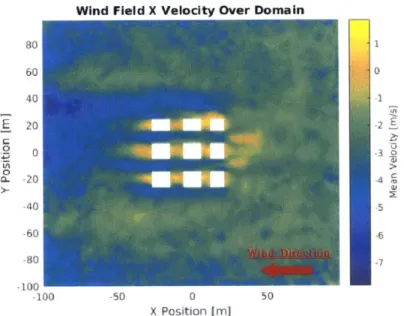
The microscale, seen in figure 1-la, considers the effect of individual objects and structures and is defined between one meter and several hundred meters. Its vertical extent is entirely contained within the roughness sublayer, and includes the urban canopy layer (UCL). The UCL extends up to the mean feature height and because urban environments are dominated by the structures within them, the mean feature height tends to also be the mean structure height. However, as the name suggests, the concept originated with the study of wind flow within forest canopies. The flow within the urban canopy layer is driven by the flow in the upper sublayers, but is strongly governed by its dense structure. Just as the terrain's interaction with the flow creates complex features at higher altitudes, the urban canopy layer contains many flow features that can have a significant effect on flight performance. The most straightforward example of a flow feature exploitable by a UAV is the tendency for the wind to be directed down an aligned urban canyon and over a perpendicular one. Examples of both of these effects can be seen in figure 1-3. As shown, the x component of the wind velocity within the urban canyons is relatively smooth and continuous, while there is a significant reduction in magnitude directly behind the structures at this altitude.

Wind Field X Velocity Over Domain 80 60 E 0 In 0 -60 -80 -100 100 -50 0 50 X Position rnmj

Figure 1-3: Example wind field estimate generated by a computational fluid dynamics

solver with the prevailing wind flowing from the right to the left. Note the lower wind velocities found in the wake regions of the buildings and the accelerated flow down the aligned canyons.

Although those examples are intuitive, the urban environment also contains more complex features such as the frontal vortexes and trailing wake regions found near single buildings, as described by Blocken et al. 1141 and shown in figure 1-4a. As discussed by Ioydysh et al. 1501 and shown in figure 1-4b. other wind features can be found in the vortexes created by the interaction of the flow around several. closely packed structures. Kittiyoungkun 1551 provides further discussion on the range of wind features found in the urban environment and their relevance to UAV flight. As all of these flow features demonstrate. the complex flow within the urban canopy layer is a challenge to estimate and care must be taken when selecting from the wide range of wind field estimation techniques.

1.3

Wind Field Estimation

Although there are many common wind field estimation techniques, no single ap-proach is well suited to all applications and environments and very few are able to capture the complexity found within urban wind fields. This section contains a brief

HORIZONTAL

VORTEX

IIrk

INTERMITTENT

CORER VORTICES

(a) Single Structure Flow Features [141 (b) Structure Group Flow Features [50]

Figure 1-4: Illustrations of the flow features found around a single structure and structure group. Note that the scales of each of these features varies with structure dimensions and some may cease to exist for certain configurations. Figures used with permission from authors.

summary of several common wind field estimation methods and their applicability to urban environments.

The simplest approach to wind field estimation is to assume a uniform wind ve-locity with intermittent gusts. The 1-cosine gust model derives from the Military

Specification MIL-F-8785C and is applied to each velocity component individually.

The inputs are the gust amplitude in meters per second, gust length in meters, and start time. Although this might be useful for testing a vehicle or structure's response to a smoothed step-input, it, does nothing to encode a wind field's natural spatial or temporal variation. A more sophisticated approach is found in the Dryden and von Karman turbulence models. Both of these use characteristic length scales and intensities to define the power spectral densities over the linear and angular compo-nents of the wind velocity. The output is a static vector field with a degree of spatial variation corresponding to the input parameters. Although these are commonly used to assess an aircraft's response to turbulent wind fields, the temporal variation is only created by the aircraft's movement through the environment and does not exist for a stationary vehicle. Although the von-Karman model is the preferred continuous gust model of both the Federal Aviation Administration and Department of Defense, neither it nor the other methods discussed thus far are applicable to low altitude wind

fields because they have no way of incorporating the terrain's effect on the flow. An alternative approach to capturing the interaction between the flow and terrain is to forgo simple models and rely solely on a set of wind measurements throughout the domain.

Meteorology was one of the earliest fields to investigate wind field estimation us-ing Krigus-ing, also called Gaussian process regression. Gaussian process regression, discussed more thoroughly by Rasmussen et al. [86], takes a series of measurements as inputs and uses a function to define the covariance between any two points. This covariance function, or kernal function, often has a set of hyperparameters that are estimated given a set of training data. The resulting kernel function defines a distri-bution over functions that generates a continuous function over the space that can be queried with a test point to get the corresponding mean and covariance estimate. This technique has much to offer when a large number of measurements are evenly distributed throughout the domain and the resulting regression is well supported over the area of interest. While these assumptions are true for wind field estimation using data from satellite scatterometry, where mesoscale wind velocities are inferred from changes in reflected radiation from the earth's surface, they do not hold in urban en-vironments due to the sparsity of measurements provided by existing weather stations or any quickly deployable system. A further complication is that the kernel functions used by the regression assume a spatial smoothness that is violated by any obstacles in the domain. These discontinuities cause the wind field estimate to incorrectly pre-dict a strong correlation between wind velocities on either side of an obstacle, when the physical separation clearly breaks any physical constraints. This failure mode constrains the approach to only being used far from obstacles that interfere with the flow behavior. More recently, Lawrance et al. [61, 62] used a variant of this approach with a time history of wind measurements along a vehicle's flight path. Their ap-proach relies on a spatio-temporal kernel to provide variable sampling density over the map and sparsification of the training set for online estimation. Despite these clever features, this approach suffers from the same drawbacks inherent in spatially smooth kernel functions in environments with obstacles.

While the complexity of the urban environment and its wind fields defeats these approaches, the dense and static structures actually provide some predictability given known prevailing wind conditions. A naive approach would be to use the publi-cally available measurements from weather stations as inputs to a simple regression. Unfortunately, the complex geometry of a typical urban environment would require weather stations at nearly every street corner to properly capture the resulting flow fields. Because weather stations tend to be distributed at the scale of neighborhoods, they cannot sufficiently capture the flow fields within the urban canyons, but are suf-ficiently dense to provide an accurate estimate of the local prevailing wind conditions in the upper sublayers. Combining these estimates with a model for the horizontal ve-locity profile and a map of the structures in the environment defines both the domain and input conditions for a computational fluid dynamics solver that can simulate the interaction of the flow with the environment. Although computationally taxing, the accuracy of this approach and its prior use in urban planning, structural engineering, and studies of fixed-wing flight performance in urban environments motivates its use for this application.

In general, CFD solvers use one of three main turbulence models to solve the Navier-Stokes equations. In order of increasing sophistication, realism, and solution complexity, these are Reynolds-averaged Navier-Stokes (RANS), large-eddy simula-tion (LES), and direct numerical simulasimula-tion (DNS). RANS provides a time-averaged or steady solution and therefore generates a static wind field estimate. Due to its relative computational simplicity, RANS is the standard in the engineering industry,

and the k - c model is the most frequently used version. This two parameter

turbu-lence model resolves the two transport equations for the turbulent kinetic energy, k, and the turbulent dissipation rate, c. Despite the popularity of RANS models, they incorrectly assume that the turbulent behavior is equivalent at all scales. Because this is not true, LES directly solves for the flow in the larger, transient, and geometry dependent eddies, but resolves the more universal and isotropic smaller scale eddies with an approximate subgrid-scale model. Since LES is used in an unsteady simula-tion, it provides a time series of wind fields by explicitly computing the time evolution

of the flow. DNS, the most computationally intensive method, directly solves for the flow at all scales. Currently, this is only feasible for very small domains and will not be considered here. Further details on CFD simulation, turbulence models, and the significant of the various approaches will be discussed later.

1.4

Minimum-Energy Trajectory Planning

As established in the literature and discussed in greater depth later, a natural way to drive the exploitation of a wind field is to consider the amount of energy being expended by the agent as it navigates through the environment. For a vehicle without wing lift, it is natural that traveling upwind should have a higher action cost than traveling downwind due to the increased form drag. A winged vehicle adds some additional complexity because the vehicle's lift must be considered along with its airspeed. A vehicle's airspeed is defined as the wind speed minus the vehicle's ground speed. The study of this problem, minimum-energy trajectories for winged vehicles, is generally called soaring and is an important reference for the work presented here.

A common practice among birds as well as manned and unmanned gliders, soaring

is the act of extracting energy from the wind field in order to improve some aspect of flight performance. In the earliest known description [5], Lord Rayleigh stated that when a bird does not work its wings while maintaining altitude, we must conclude that either the wind is not horizontal, or the wind is not uniform. These two alterna-tives are now known as static and dynamic soaring, respectively. Specifically, static soaring is the extraction of energy, usually in the form of potential energy, from a relatively uniform wind feature that provides lift through the vertical component of the wind velocity. Dynamic soaring is the extraction of energy from large gradients in the wind field such as those created by waves or hills and frequently exploited by albatrosses [95]. Both types share the common objective of extending flight range or duration. Despite its frequent use in nature as well as manned, fixed-wing flight, the effective use of soaring has yet to be demonstrated in complex wind fields such as those found in urban environments. Although the fixed surfaces of a quadrotor cannot

generate much lift, the minimum-energy trajectory planning approaches developed in the soaring literature offer an appropriate foundation for the work presented here.

1.5

Overview

This document begins with Chapter 2 by discussing related work in wind field esti-mation for UAV flight, trajectory planning for fixed-wing UAV soaring, and past ap-proaches to on-board wind velocity measurement. The remainder of the work presents results from two distinct efforts to enable quadrotors to efficiently and safely navigate the complex wind fields found in urban environments. The first component focuses on wind field estimation and begins in Chapter 3 with the design, development, and testing of a low-cost wind sensor for two-dimensional wind velocity measurement on-board a quadrotor. This leads into Chapter 4 with a discussion of urban wind field simulation using a CFD solver. Chapter 5 presents the second component which analyzes a quadrotor's ability to exploit urban wind fields for improved flight perfor-mance. This includes a formal planning problem statement, the development of an empirically derived power consumption model, and discusses the simulation results of minimum-energy trajectory planning over portions of the MIT campus with known wind fields. Finally, Chapter 6 closes with conclusions.

Chapter 2

Related Work

The related work presented here draws from the research areas of fixed-wing UAV soaring, analyses of UAV flight performance in urban wind fields, and on-board wind estimation. Although a few of these efforts have focused on single and multi-rotor UAVs, the majority of the supporting literature comes from research on fixed-wing platforms. For clarity, the relevant components of each work have been arranged into the sections on wind field estimation, trajectory planning, and on-board wind estimation.

2.1

Wind Field Estimation

A prerequisite for exploiting a wind field is having an accurate estimate of that wind

field. The simplest approach, demonstrated by Ceccarelli et al. [22] and Osborne et al. [81], is to assume that it is both static and uniform. Although this might be a decent approximation for an instantaneous snapshot of a synoptic wind field at high altitude, it ignores the dynamic nature of weather patterns and could become arbi-trarily wrong as the prevailing wind shifts. Providing an incremental improvement,

Rysdyk et al. [94] and Langelaan et al.

158]

pre-vailing wind vector with additive Gaussian noise. A series of air and ground speed measurements are then used to estimate each component of the prevailing wind veloc-ity. Although this approach allows for slowly evolving, uniform wind fields, it forces

the user to choose between robustness and accuracy in the complex wind fields found at lower altitudes where the terrain's influence on the wind field creates spatial and temporal variation. Despite its drawbacks, the method of using a history of local measurements to build a global wind field estimate is one frequently taken in the soaring literature.

2.1.1

Local Measurements

Using a set of local measurements can be a flexible and powerful approach to wind field estimation, but imposes strong constraints on the quality and distribution of those measurements. As might be expected, given an expressive representation and a sufficient number of wind measurements appropriately distributed throughout the domain, the global estimate obtained from the measurement set could closely ap-proximate the true wind field. However, an overly sparse or poorly distributed set of samples over the domain could artificially and erroneously bias the resulting estimate. One example of using a history of local measurements to estimate the global wind

field was presented by Langelaan et al.

[59],

parameteri-zation of the wind velocity over altitude. Given wind velocity measurements from a Pitot tube mounted on a small, powered glider, a Kalman filter was used to estimate the polynomial coefficients of the horizontal wind speed profile. By repeatedly flying vertical loops, the estimate of the velocity profile was updated with the new mea-surements and propagated with a constant motion model between time steps. The evolving velocity profile can be seen in figure 2-1. A similar approach was taken by

Sydney et al.

[1001

spatially varying wind field while estimating the values of a parametric wind model using a recursive Bayesian filter. Although these techniques allow both temporal and spatial variation in the wind field, they solve both of these problems in overly simpli-fied ways such that the generated estimates are not expressive enough to be used in more general environments.

Working with a powered motor-glider, Allen [7] used a history of wind speed and

lift rate measurements to estimate thermal location, size, and strength. Each of these

jj 0400

/

I 3 4

Figure 2-1: Langelaan et al.

[59]

parameters was found by using gradient descent to fit a spatial. squared exponential model of the wind velocity over the weighted history of measurements. A total of

23 thermals were detected and utilized over the course of 17 flights with an average

altitude gain of 173 m. The flight, path data from one of these flights can be seen in figure 2-2. Although this approach allowed for the successful discovery and tracking of thermals, it achieved this success by placing strong assumptions on the form of the wind field and then only flying near these wind features. In order to be successful outside of this narrow application, the method must allow for wind fields of a more general form.

In [61., 62]. Lawrance et al. presented a wind field estimation technique that relies on Gaussian process regression over a history of local measurements and demonstrated its ability to build an accurate estimate of a static wind field with a single, stationary thermal. This nonparametric approach is powerful because it can use a set of wind measurements over the map to build a continuous estimate of an arbitrary wind field. Accordingly. this method captures spatial variation quite well, but does not

-700 5.0 Aircraft path 4.5 Estimated thermal center -800 4. Start . Finish -900 3.0 2.5 PX in -1000 20 1.5 -1100 1.0 0.5 -1200 0 -0.5 -1300 -1.0 -100 0 1 A 200 300 40 300 -.

Figure 2-2: A figure from Allen

I7I

elegantly handle temporal variation. For example, a temporal drift in a static wind field would require heavy resampling to get an accurate estimate of the shifted., but otherwise unchanged, wind field. Another drawback of this approach is its cubic complexity with respect to the number of measurements over every optimization step while learning the hyperparameters that define the covariance kernel function. Given the innate need to collect online measurements, the size of the measurement history must be carefully managed and places an upper bound on the resulting estimate's maximum domain size and resolution. An example of a wind field estimate from this approach can be seen in figure 2-3. This estimate is from a simulation of a glider exploring a 400 m x 200 in x 100 in domain with no initial knowledge of the wind field. Accordingly, there is an initial period while the domain is being explored before the estimate closely approximates the true wind field. Note that the domain size is relatively small relative to the scales of high altitude wind features being exploited in

typical fixed-wind soaring.

Also note that the simulation in figure 2-3 exaggerates the Gaussian process's ability to estimate complex spatial variation by including the sinusoidal wind feature across the domain. In general., it is challenging to infer the state of the wind field at a distance from the current measurement location, but including the rarely found,

30

O 0.2 0 0 4 0 C

200.7 -10

40024m

'0 ~ .~ $ '100 00 3 00

Om 10 2000

Figure 2-3: An illustration from Lawrance et al. [61] of the ground truth, shown on the left. and final mean estiniate, shown on the right, of the wind field in a domain with a Lee wave and thermal. The cone's size and orientation represent the wind speed and direction. respectively, and are color coded by the variance in (m/s)2. The

red crosses indicate the vehicle fiight path through the environment. Figures used

with perinssion from authors.

periodic Lee wave somewhat artificially enables local measurements to be accurately

propagated over one dimension of the domain. If the wind field were composed of a dense set of more spatially irregular features, significantly more measurements would be required to get the same accuracy. This case would further complicate the challenge of tuning the length scale paraneters of the squared exponential kernel function. Without, a regular set of features with known length scales, it would be easy to overfit to a particular feature and smooth over higher frequency variation present in another.

In an attempt to address some of these issues, Lawrance et al. modify their approach in 1631 to allow for timle varying wind fields and feature drift. The spatio-temporal kernel proposed in their work also gives a relatively rigorous method for rejecting the least informative measurements in the set. As previously mentioned, this is a critical factor in managing the complexity of updating the estimate. A time series of wind field estimates and their corresponding glider trajectory for a single simulation can be seen in figure 2-4. Again, despite the more sophisticated kernel function. the size of the domain is relatively small compared to typical glider flight paths. By continuing to rely on the periodic Lee wave as the central wind feature, this work also underestimates the number of measurements needed for an accurate

-0 0

(m t 2-5O-s actual wi d ield

10- :

S i250 path taken Mid current wind estimate

1k

(h 4250t Iwidtil

10400

d1 4

(d) 5 pat iken anrd currenti wind esimaitre

Figure 2-4: A series of snapshots of the wind field estimate and flight path from a simulation done by Lawrance et al. 1631. The path is indicated by the grey line and the

autonomous soaring begins at the green triangle after an initial period of exploration and ends at the red circle. The cones represent the wind velocity magnitude and heading and are color coded by the variance in (rI/s)2. Figures used with permission from authors.

0

estimate in a, more irregular wind field.

More fundamentally, Lawrance et al.

[631

growth in computational complexity of updating the wind field estimate as the num-ber of measurements increased. The relatively large amount of spatial variation in a similarly sized urban wind field would significantly increase the number of mea-surements required to accurately capture the underlying wind field. The temporal variation at any point, would also prevent a single measurement from being represen-tative of the expected wind velocity and would require repeated visits or extended periods of time to be spent at every measurement location. Finally, there is an inher-ent assumption of smoothness when using any common kernel function such as the squared-exponential. Urban wind fields violate this assumption because the

struc-32 400

tures in the urban environment introduce sharp discontinuities within the domain. For example, a measurement on one side of a building corner is only loosely corre-lated with the conditions on the opposite side. A measurement upstream of a small obstacle compared with one downstream also has little correlation, despite its close spatial proximity. With these limitations in mind, it becomes clear that any success-ful approach to urban wind field estimation will explicitly incorporate a model of the

environment or similar environments in some way.

2.1.2

Simulation

A more direct approach to wind field estimation uses CFD and a model of the

environ-ment to simulate the wind fields generated by the current prevailing wind and weather conditions. Recently, several authors have made significant headway in applying CFD solvers to wind field estimation for UAV flight. The following section outlines their results and investigates the strengths and weaknesses of their approaches in regard to urban wind field estimation.

Chakrabarty and Langelaan [24] demonstrated the use of CFD for wind field es-timation for a fixed-wing, unpowered glider path planning over a mountain range in central Pennsylvania during a 12 hour period on October 7, 2007. The simulated glider was a RnR Products SB-XC with a mass of 10 kg and a roughly 4 m wing span. The objective was to extend the vehicle's range as it attempted to reach a goal by exploiting regions of lift within the wind field. The time series of wind field

estimates was computed by Young et al.

[108]

package Weather Research and Forecasting (WRF). The simulation domain had a large extent of 70 km x 70 km x 5 km with a discretization of 0.44 km horizontally and a descending density with increasing altitude. Unlike using a history of local mea-surements, CFD solvers directly compute global wind fields that explicitly consider the effect of the terrain. Although CFD solvers are computationally expensive, the results are more likely to be accurate, and assuming offline computation, significantly larger domains can be considered. To extend the use of a CFD solver to a real-time application with arbitrary prevailing wind conditions, a library of wind fields would

5 41 4 60 0 6050 20 iia m 0 40 0u 10 (iOhkim 0 0 o ( north Lum U it km Oo 4 S. ) 1=1 X)h UT1'C (b t115h UC 0 0 60 60 (, 0M0 _{20 0 oo} 50 _io 6

north ki ) 10 0 0 - 114)1ea kil 0 0 k20

(C) t=1301 UTC (d) t=1 145h UTC

Figure 2-5: Simulation results from Chakrabarty and LangelaanJ24] showing four snapshots in time over the course of the flight. Note that the vehicle follows the color coded lift regions as they evolve over time. Figures used with permnission from authors.

need to be precomputed and stored for a spanning set of prevailing wind speeds and headings. Although the use of a numerical solver for wind field estimation that ex-plicit considers the terrain offers promise for obtaining urban wind field estimates, the WRF cannot handle the dense structure of urban environments. Fortunately, other

CFD packages offer suitable alternatives.

Although no previous results have addressed planning over urban wind fields, sev-eral efforts have been made to generate wind fields using CFD solvers to characterize tieir effect on UAV flight performance. Galway et al. [43, 40., 41, 42] investigated the effect of wind fields within a sparse urban environment on the path following

perfor-mance and control effort of both a single-rotor and fixed-wing UAV. In an effort to avoid recomputing the wind field for every new environment, a library of 3D wind field

primitives was built, using the ANSYS CFX CFD package. The library was composed 34

2. 2i I 2 2 22 '2> -IL 2 1 }

KK

Figure 2-6: Two 2D vector plots showing wind fields on a horizontal plane at half the structure height from the 3D simulation environment used in Galway et al.

[42].

in the direction of the arrow heads with white being higher speeds and black being lower speeds. Note the interaction between the two structures on the right that acts to speed up the flow through the canyon. Figures used with permission from authors.

of wind fields for small groups of structures with one or two buildings over a set of prevailing wind conditions. The objective of the work was to combine these wind field primitives to generate an accurate estimate over a more complex environment with many structures. An example of these wind field solutions can be seen in figure 2-6.

Each of these wind fields was computed using an unsteady LES simulation with a 0.1 s time step over a total of 20 s. The resulting time series of wind fields was then post processed to find a bounding wake region that contained the time varying portion of the wind field. Once this wake region was identified, it could be directly

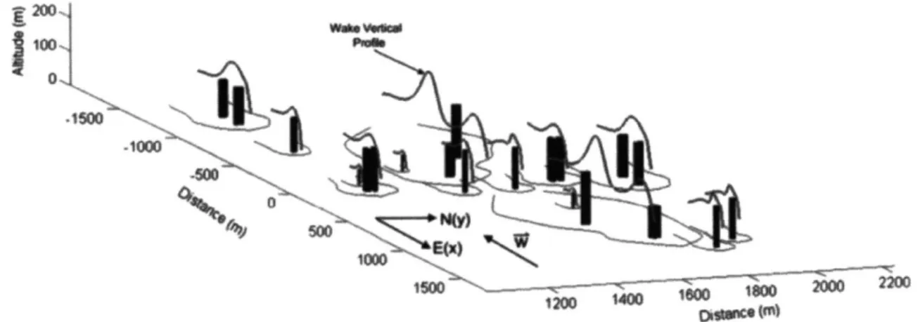
2001 A WC 10 1000

Iio

Figure 2-7: An illustration of the 3D simulation environment used in Galway et al.

[42].

combined with other elements of the library as long as their wake regions did not overlap. Further work was done to combine wind fields with overlapping wake regions in special cases. An example of a wind field composed of many library elements, some of which overlap, can be see in figure 2-7.

By simulating the vehicle's flight along a given target trajectory through a

pre-computed wind field unknown to the vehicle, Galway et al. further demonstrated that the forces generated by the vehicle's interaction with the wind field had a sig-nificant effect on the control effort and trajectory following performance of both the single-rotor and fixed-wing UAV. Although Galway's approach allows for approximate wind fields to be generated for this specific subset of sparse urban environments with building groups no larger than one or two structures, these constraints on structure density and geometry prevent the approach from capturing wind fields in more com-plex and dense environments found at ground level in a typical city. Although no attempt at trajectory planning was made in this work, it is also unclear how a raw unsteady wind field simulation would be used in a planner because even a wind field with a dominantly periodic evolution would need to be synchronized with the current conditions.

Orr et al. [80] and Gross et al. 147] made several efforts investigating UAV flight in

36

urban environments through an Air Force Research Laboratory (AFRL) project called the Cooperative Operations in Urban Terrain (COUNTER). This work focused on the effect of wind fields over a small group of buildings on a fixed-wing UAV's ability to reach a set of waypoints. The fixed-wing UAV used in simulation for this work had a mass of 9.5 kg, a wing span of 1.8 m, and a cruising speed of 13 m/s. The simulation domain was a small grouping of 15 structures that composed a town square. The tallest of the structures was three stories. Steady wind field simulation was done with a CFD package called the Air Vehicles Unstructured Solver (AVUS). The simulated wind field had a prevailing wind speed of 4.6 m/s and southerly heading and although no detailed analysis was presented on the effects of the wind field on the vehicle's path following performance, it was noted that the addition of the wind field prevented the

UAV from reaching several of the waypoints in its path. In this case, the addition of

the wind field into the simulation caused the vehicle to exceed its maximum airspeed along the target trajectory and forced it to abandon the unreachable waypoints.

Similar to the work of Chakrabarty et al [241 and Galway et al.

143,

the approach taken by Orr et al.

[80]

[47]

considering the effect of the terrain on the wind field. However, relative to our appli-cation, it improved upon these approaches by doing so for a dense urban environment without the need to combine wind field primitives. A potential drawback lies in the questionable ability of a steady CFD solver to accurately capture the unsteadiness present in an urban environment. Although it might be able to capture the mean flow velocities, it does not provide any uncertainty estimate over the map.

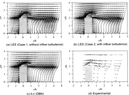
White et al. [1031 used steady and unsteady CFD simulation as well as wind tun-nel and in-situ measurements to investigate the ability of a small fixed-wing glider to soar in the rear wake region of a structure. The wind vectors over a vertical 2D plan can be seen in figure 2-8 and show good agreement between the measured data

and simulation data. Notably, the steady k - E RANS solution has strong agreement

with the wind tunnel measurements, and the LES simulation required the inclusion of inflow turbulence to match these results. Given the fixed-wing UAV's lift character-istics found in a separate wind tunnel experiment, it was determined that this UAV

JA _7

(a) LES (Case 1: without infow turbulence) (b) LES (Case 2; with inflow turbulence)

(c) k-c (DBN) (d) Experimental

Figure 2-8: White et al. [1031 presents the velocity vectors from numerical simulations comparing the RANS and LES turbulence models (a-c) and the in-situ experimental data (d). Note the similarity between the RANS simulation and the LES simulation with the modeled inflow turbulence. Figures used with permission from authors.

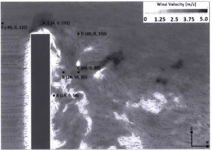
would be able to effectively soar in the wake region of this building. Unfortunately, no planning or flight simulations were performed to justify this conclusion, but this work remains an example of the ability of CFD simulation to compute accurate estimates of complex wind fields close to structures at the resolutions necessary for UAV flight. Sutherland [99] also studied UAV flight performance in the wake region of a single structure, but focused on quadrotor flight performance while investigating the effec-tive differences between using a RANS and LES turbulence model. This work used the OpenFOAM CFD solver to generate a set of wind fields around a single structure with dimensions 20 x 20 x 120 ni. In an effort to ensure the accuracy of the wind field estimates, much of this work was directed towards a series of sensitivity analyses on spatial and temporal resolution as well as verification studies. As in Galway et al.[42j, a wind field database was constructed in order to decouple the 30 s runtime of the flight simulation and the 0.97 and 17.7 hour wind field computation time for the RANS and LES models, respectively. Once the wind field library was built, it was used to analyze the performance of a quadrotor position controller in various locations around the structure for both CFD methods. In summary, the LES

Wind Velocity [rn/si

E( 3 0 1.25 2.5 3.75 5.0

D 40, 0, 120)

61(24, 6, 80i 7

A (14. 0, 56)

Figure 2-9: Raza and Etele [871 show a vector field from a wind simulation of the flow around a single structure and the trajectory waypoints in their simulation. Figures used with permission from authors.

lations did significantly better resolving the innately unsteady turbulent fluctuations and therefore its wind fields had a more significant effect on the quadrotor's flight per-formance. Sutherland also notes that, the additional complexity of LES means that it should primarily be used in the pursuit of designing and testing autonomous control algorithms for nultirotor UAVs on the order of 0.5 m in size and 2 kg in mass. Build-ing further on these results, Raza and Etele 187] used the same wind field database to characterize the performance of several quadrotor position controllers while flying in the structure's wake region. Again, these authors concluded that LES was superior to RANS in its ability to accurately model the smaller-scale perturbations placed on the quadrotor due to turbulence, but also resulted in significantly increased solution times.

Cybyk et al. [31j performed a similar investigation into the effects of wind fields on fixed-wing flight performance over a nultikilometer portion of Baghdad, Iraq. The terrain geometry was resolved to 1 in and the wind field to 6 m resolution.

The unsteady, LES wind fields were generated with the FAST3D-CT CFD package.

Harms et al. [49] presented a validation study of FAST3D-CT against the data from a large field trial in Oklahoma City summarized in work by Allwine et al. [10, 8 9, 16].

4/

NA

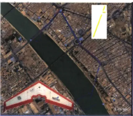
Figure 2-10: An illustration from Cybyk et al. [311 of the Procerus Unicorn UAS and the simulated mission route through downtown Baghdad with a prevailing wind

head-ing of 20 degrees and prevailhead-ing wind speed of 3 m 's. Figures used with permission from authors.

The UAV used in simulation was the Procerus Unicorn, a powered glider with a 1 m wing span that weighs approximately 2 kg. An example trajectory from a single simulation along with an image of the UAV is shown in figure 2-10. This trajectory was simulated without wind., with a 3 m1 s prevailing wind speed using only translational

wind velocity, and with a 3 m/s prevailing wind speed with both translational and rotational wind velocities. Although no planning was done and a detailed analysis of the UAV's flight performance was not performed, these few trajectories generated significant differences in the vehicle's control effort. position., and attitude.

In a slightly different application, the Navy has used both RANS and LES CFD

solvers to estimate wind fields near structures for flight simulation and the analysis of helicopter and fixed-wing flight perforniance. Bogstad et al. [15], Zan [1091, and Forrest et al. [371 used CFD to create an extensive airwake database for a ship-specific flight simulator to train helicopter pilots for landing and takeoff from various points on a ship. Similarly, Crozon et al. [30] used CFD to analyze the interaction

40

I

between the rotor and the frigate deck in a single simulation.

2.2

Minimum-Energy Planning

A critical component of the quadrotor's ability to exploit an urban wind field for

improved flight performance is a planner that will choose the appropriate path through the environment. The soaring community has thoroughly addressed this problem using minimum-energy trajectory planning for its ability to encode the desire not only to avoid flying into headwinds and catch tailwinds, but to provide vertical lift and exploit shear layers in the wind field. Although a quadrotor cannot generate lift as efficiently as a fixed-wing vehicle, the same inherent connection exists between a minimum-energy trajectory and the ability to efficiently fly through wind fields. The following section presents the relevant details of closely related work from the soaring community that informed our planning algorithm.

Chakrabarty et al. [23] developed a graph-based planning method that uses A* search to plan over the domain using a feasible action set. The edge cost is the energy consumption along that edge in the graph. A weighting between the Euclidean distance heuristic and energy consumption is proposed to tune the behavior of the planner. Figure 2-11 shows the behavior of the planner for different weightings of the heuristic over a simple domain.

In an extension of this work, Chakrabarty et al.

124]

complex wind fields over a mountain range. Although the wind field estimation com-ponent of this work was previously discussed, this is also one of the few examples of UAV path planning in time-varying wind fields. To circumvent the complexity of planning over time varying wind fields, a kinematic tree algorithm, originally

pre-sented in Langelaan

[57],

receding horizon framework. This planning approach minimizes the distance to the goal while maximizing the total energy.

7 500 0 100 -80 \kil 60 AA 40 - alpha = 0.95 4 - alpha = 0.96 - alpha = 0.97 20 - alpha = 0.98 - alpha = 0.99 0 0 10 20 alpha = 1.00 _{x (kil} energy map

Figure 2-11: A comparison from Chakrabarty et al. 123] of A* paths with varying weights on inimuni-distance and energy consumption along with the ideal path through this environment and cost map. Figures used with permission from authors.

2.3

Wind Measurement

Although it is not yet clear how to incorporate on-board wind velocity measurements into a wind field estimate, it is intuitive that an accurate local measurement could provide useful information for a trajectory planner or wind field estimation algorithm. This is reinforced by the work of Alexander and Vogel 16] which investigated the ability of several species of birds to align themselves with their intended direction of travel and mitigate the effects of wind gusts using measurements of the wind velocity along their flight trajectory. Additional work was done by Gewecke and Woike 144] and Brown and Fedde 119] demonstrating the connection between the airflow over avian feathers and the bird's steering impulses as well as the ability to predict stall and measure airspeed. Local wind measurements could also provide a check on the accuracy of the current global wind field estimate within that region of the map. The following section presents the relevant details of closely related work from the UAV community on on-board wind velocity estimation and measurement. A few of these efforts have focused on single-rotor MAVs, but the majority of the work considers fixed-wing vehicles.

42