Field Assessment of the Thermal Characteristics of Innovative Glazing Systems at the Canadian Centre for Housing Technology

(1)

https://doi.org/10.4224/20377183

READ THESE TERMS AND CONDITIONS CAREFULLY BEFORE USING THIS WEBSITE. https://nrc-publications.canada.ca/eng/copyright

Questions? Contact the NRC Publications Archive team at

PublicationsArchive-ArchivesPublications@nrc-cnrc.gc.ca. If you wish to email the authors directly, please see the first page of the publication for their contact information.

NRC Publications Archive

Archives des publications du CNRC

For the publisher’s version, please access the DOI link below./ Pour consulter la version de l’éditeur, utilisez le lien DOI ci-dessous.

Access and use of this website and the material on it are subject to the Terms and Conditions set forth at

Field Assessment of the Thermal Characteristics of Innovative Glazing

Systems at the Canadian Centre for Housing Technology

Manning, M. M.; Elmahdy, A. H.; Swinton, M. C.; Szadkowski, F.

https://publications-cnrc.canada.ca/fra/droits

L’accès à ce site Web et l’utilisation de son contenu sont assujettis aux conditions présentées dans le site

LISEZ CES CONDITIONS ATTENTIVEMENT AVANT D’UTILISER CE SITE WEB.

NRC Publications Record / Notice d'Archives des publications de CNRC:

https://nrc-publications.canada.ca/eng/view/object/?id=2710ac84-845b-4d59-820a-3bea0e376dfd https://publications-cnrc.canada.ca/fra/voir/objet/?id=2710ac84-845b-4d59-820a-3bea0e376dfd

(2)

Canadian

Centre

canadien

des

for Housing Technology

technologies résidentielles

Final Report

FIELD ASSESSMENT OF THE THERMAL CHARACTERISTICS OF

INNOVATIVE GLAZING SYSTEMS AT

THE CANADIAN CENTRE FOR HOUSING TECHNOLOGY

Contract: B-1248

Manning, M.M.; Parekh, A.; Elmahdy, A. H.;

Swinton, M.C.; Szadkowski, F.

(3)

The Canadian Centre for Housing Technology (CCHT)

Built in 1998, the Canadian Centre for Housing Technology (CCHT) is jointly operated by the National Research Council, Natural Resources Canada, and Canada Mortgage and Housing Corporation. CCHT's mission is to accelerate the development of new technologies and their acceptance in the marketplace.

The Canadian Centre for Housing Technology features twin research houses to evaluate the whole-house performance of new technologies in side-by-side testing. The twin houses offer an intensively monitored real-world environment with simulated occupancy to assess the performance of the residential energy technologies in secure premises. This facility was designed to provide a stepping-stone for manufacturers and developers to test innovative technologies prior to full field trials in occupied houses.

As well, CCHT has an information centre, the InfoCentre, which features a showroom, high-tech meeting room, and the CMHC award winning FlexHouse™ design, shown at CCHT as a demo home. The InfoCentre also features functioning state-of-the art equipment, and demo solar photovoltaic panels. There are over 50 meetings and tours at CCHT annually, with presentations and visits occurring with national and international visitors on a regular basis.

(4)

Acknowledgements

Thanks are extended to Chris Barry of Pilkington North America for providing partial funding for this project and expert advice. Thanks are also extended to Sylvain Harnay and Roger Marchand for their assistance with instrumentation and documentation.

Acronyms

ach – air changes per hour cfm – cubic feet per minute

CVD – chemical vapour deposition HRV – Heat Recovery Ventilator HSG – High Solar Gain

LSG – Low Solar Gain

CCHT - Canadian Centre for Housing Technology CMHC - Canada Mortgage and Housing Corporation NRC - National Research Council Canada

NRCan - Natural Resources Canada

(5)

Executive Summary

The impact on house energy consumption of changing the solar heat gain characteristics of glazing systems from “High Solar Heat Gain” (HSG) to “Low Solar Heat Gain” (LSG) was studied both experimentally and by energy analysis. The experimental work was performed in the twin houses of the Canadian Center for Housing Technology (CCHT) located on the National Research Council of Canada (NRC) Campus in Ottawa, Ontario. NRCan staff, using RESFEN, HOT2000 and ESPr computer programs, performed the analytical work.

The LSG and HSG glazing were compared for 28 days during the winter (19 January to 15 February, 2006) and 23 days during the summer (7 July to 1 August). During these periods, all 31 glazing units in the CCHT Test House were replaced with LSG glazing and compared to 31 HSG glazed windows in the Reference House. The impact of the glazing on solar gains, heating and air conditioning energy consumption, window surface temperatures and room temperatures was monitored.

The evaluated HSG product had a nominal centre of glass U-factor of 1.65 W/m2°K, and a nominal SHGC = 0.72. The LSG product had a nominal centre of glass U-factor of 1.36 W/m2°K and a nominal SHGC=0.41,

Measurements of solar transmission indicated that the LSG glazing transmits ~40% of the total radiation on a sunny winter day, while the HSG glazing transmits ~60%. Because of the reduced solar gains during the winter evaluation, the LSG glazing caused the house to consume on average 23/MJ/day (8.7%) more natural gas for heating and 0.13 kWh/day (1.3%) more electricity for the furnace fan blower, than the HSG glazing. In summer, the LSG glazing continued to introduce less solar gains to the house than the HSG glazing, and thus produced savings in cooling energy of 14.7 MJ/day (17.7%) on average.

The interior surface of the HSG windows reached higher temperatures than the interior surface of the LSG windows on days with high solar gains. The effect was most pronounced during winter, when the sun was lower in the sky and at a smaller angle to the window surface. South facing HSG windows were up to 12.3°C warmer on the inner surface in winter, and 7.9°C warmer in summer. South facing room temperatures with the HSG glazing were up to 3.8°C warmer at mid-height on sunny winter days, and up to 1.0°C warmer on sunny summer days.

Using experimental relationships between solar transmission and consumption, the field trial results were projected to the full year. Annually, the HSG glazing produced a total of 3015 MJ of energy savings at the CCHT facility, compared to the LSG glazing. This is equivalent to an annual cost savings of $26, assuming 2006 utility prices of $0.52/m3 of natural gas and $0.10/kWh electricity

(6)

The computer simulation was extended to cover the full year using the weather data for several cities in Canada and USA. The LSG glazing provided the best energy savings during the cooling season, and the HSG glazing provided the best energy savings during the heating season. Generally, in locations with more than 3,000 Celsius heating degree days, the HSG window produced the better energy efficiency performance.

In all locations, both the LSG and HSG provided improved energy performance over the standard double-glazing air-filled window. In all 10 locations selected in Canada, the HSG windows offer 13% to 17% reductions in annual energy costs compared to conventional windows with energy cost savings range from $117 to about $354 per year. The LSG windows offer 8% to 10% cost savings compared to conventional windows with energy cost savings range from $71 to $203 per year.

(7)

List of Tables

Table 1 - Twin House Characteristics ... 20

Table 2 Operating Conditions for the Standard CCHT Benchmark ... 20

Table 3 - Maximum Differences in Room Temperature due to the Glazing Technology, Winter Results... 42

Table 4 - Maximum Differences in Room Temperature due to the Glazing Technology, Summer Results ...58

Table 5 - Total Calculated Annual Consumption and Cost from the use of Glazing Technologies in the CCHT Test House (Nov 2005 to Oct 2006) ... 62

Table 6 - Measured monthly energy consumptions for the space heating and cooling of CCHT Reference House ... 67

Table 7 - House air tightness data after the replacement of glazing units. ... 69

Table 8 - Thermal and solar optical properties windows in CCHT houses. ... 71

Table 10 - Area-weighted average of U-factor and SHGC of CCHT windows... 73

Table 11 - Summary of measured and predicted differences in energy use during the test periods. ... 76

Table 12 - Annual space heating energy analysis of Reference and Test Houses... 77

Table 13 - Annual space cooling energy analysis of Reference and Test Houses. ... 81

Table 14 - Estimated annual energy costs for CCHT houses in year 2005. ... 82

Table 15 - Utility costs of natural gas and electricity (averaged for Nov 2006 – Feb 2007) ... 84

Table 15 - Effects of conventional, high-solar and low-solar glazing windows on annual energy use ………...86

Table 16 - Effects of conventional, high-solar and low-solar glazing windows on annual energy use and energy costs….………...87

Table A-1 - A summary of the CCHT simulated occupancy schedule ... 98

Table E-1 – Summary of CCHT Window Properties ... 110

Table I-1 - Winter 2006 Results from Glazing Field Trial ... 120

(10)

Table of Figures

Figure 1 - A schematic diagram showing the different tasks in the project ... 14

Figure 2 - Illustration of the glazing systems, with example peak window surface temperatures on clear days in summer and winter ... 17

Figure 3 - CCHT Twin-House Facility - Control House (left) and Experimental House (right)...19

Figure 4 - Precision Spectral Pyranometer mounted in the Test House south-facing bedroom window...23

Figure 5 - Window Thermocouple locations... 24

Figure 6 - Four orientations of the Research House, showing instrumented window locations... 24

Figure 7 - Range of Outdoor Temperatures during Winter ... 26

Figure 8 - Solar Radiation Incident on a Vertical South-facing surface, during winter .... 26

Figure 9 - Winter Benchmarking Furnace Gas Consumption Curve before and after the experiment. ...27

Figure 10 - Winter Furnace Gas Consumption ... 29

Figure 11 - Winter Furnace Blower Motor Electrical Consumption ... 29

Figure 12 - Transmitted Solar Energy during Winter Glazing Experiment ... 31

Figure 13 - Daily Solar Radiation Measured in the room as a function of Daily Solar Radiation Measured at the South Face of the Houses ... 31

Figure 14 - Daily Solar Radiation Measured as a Percentage of Daily Solar Radiation Measured at the South Face of the Houses ... 32

Figure 15 - Relationship between Gas Consumption and Total Incident Daily Vertical Solar Radiation ... 33

Figure 16 - Relationship between Increase in Furnace Gas Consumption and Decrease in Transmitted Solar Radiation... 34

Figure 17 - Main Floor Thermostat Temperatures ... 35

Figure 18 – Nighttime Furnace Gas Consumption (from 10 p.m. to 6 a.m.) ... 36

Figure 19 - South-facing Window Surface Temperatures ... 37

Figure 20 - South facing window surface temperature during benchmarking ... 38

Figure 21 - South facing window maximum daily temperatures during benchmarking ... 38

Figure 22 - South facing window temperatures during the window glazing experiment . 39 Figure 23 - South facing window maximum daily temperatures during the window glazing experiment ...40

Figure 24 - Sample Livingroom Ceiling Temperatures during the Winter Glazing Experiment... 41

Figure 25 - Winter Maximum Daily Temperatures at Ceiling Level in the Living room (1st Floor)...42

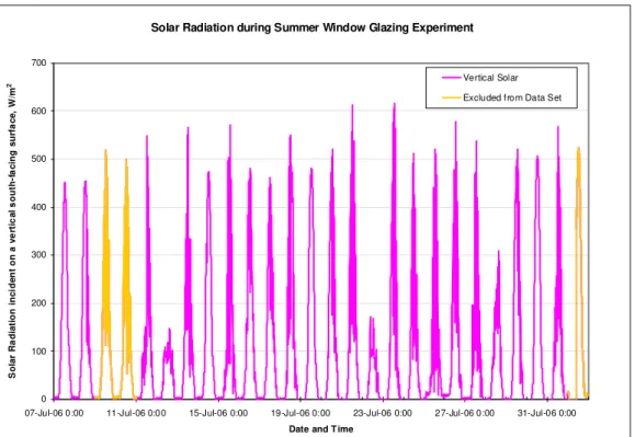
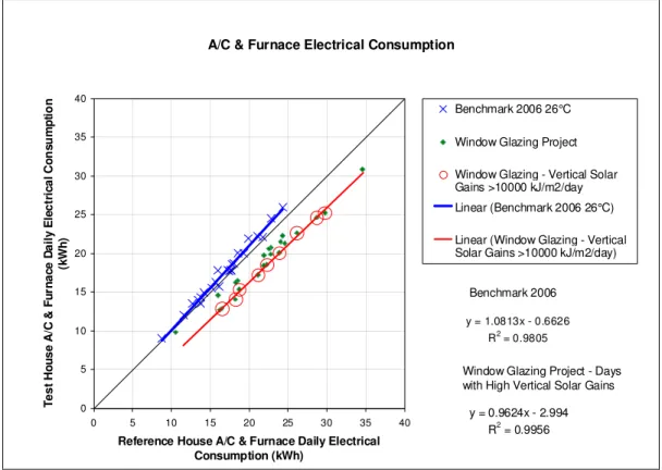
Figure 26 - Range of Outdoor Temperatures during Summer Trials ... 43

Figure 27 - Solar Radiation Incident on a Vertical South-facing surface, during Summer Trials ...44

Figure 28 - Summer benchmarking - A/C & Furnace Consumption Curve before and after the experiment ...45

Figure 29 - Window Glazing Project Summer Cooling System Electrical Consumption . 46 Figure 30 - Window Glazing Project Summer Cooling System Electrical Consumption, showing sunny day trend ... 47

Figure 31 - Transmitted Solar Energy during Summer Glazing Experiment ... 48

Figure 32 - Daily Solar Radiation Measured in the room as a function of Daily Solar Radiation Measured at the South Face of the Houses ... 49

(11)

Figure 33 - Daily Solar Radiation Measured as a Percentage of Daily Solar Radiation

Measured at the South Face of the Houses ... 49

Figure 34 - Transmission of Solar Energy on a Clear Summer Day ... 50

Figure 35 - Transmission of Solar Energy on a Cloudy Summer Day ... 50

Figure 36 - Relationship between Cooling Electrical Consumption and Total Incident Daily Vertical Solar Radiation ... 51

Figure 37 - Relationship between Decrease in Cooling Energy Consumption and Decrease in Transmitted Solar Radiation ...52

Figure 38 - South facing window surface temperature during summer benchmarking ... 53

Figure 39 - South facing window maximum daily temperatures during summer benchmarking ... 53

Figure 40 – Summer South facing window temperatures, Exterior Surface ... 54

Figure 41 - Summer South facing window temperatures, Interior Surface ... 55

Figure 42 - South facing window maximum daily temperatures during the summer window glazing experiment... 55

Figure 43 - Sample Livingroom Ceiling Temperatures during the Summer Glazing Experiment... 57

Figure 44 - Summer Maximum Daily Temperatures at Ceiling Level in the Living room (1st Floor)... 57

Figure 45 - Relationships between change in Cooling and Heating consumption and Incident Vertical Solar Radiation... 59

Figure 46 - Relationships between change in Cooling and Heating consumption and Transmitted Solar Radiation ... 60

Figure 47 - Annual projection of results: Difference in heating and cooling consumption ... 61

Figure 48 - Annual projection of results: Difference in cost of heating and cooling ... 61

Figure 49 - Cost analysis for Ottawa, based on projection of experimental results ... 62

Figure 50 - Estimates of components of cooling loads for the Reference House. ... 67

Figure 51 - Comparison of measured and estimated monthly space heating energy consumption for the Reference House. ... 68

Figure 52 - Comparison of measured and estimated monthly space cooling energy use for the Reference House... 68

Figure 53 - Profile of solar heat gain coefficient with the angle of incidence of solar rays on windows. Glazing assembly simulated using the LBNL’s Windows 5.2 for Analyzing Window Thermal Performance... 71

Figure 54 - Range of heat transfer coefficient of windows in CCHT houses... 72

Figure 55 - Effects of level of argon-fill on the heat transfer coefficient, U-factor. ... 72

Figure 56 - Energy Ratings of low solar and high solar windows... 73

Figure 57 - Average Energy Ratings of low solar (LS) and high solar (HS) windows. .... 74

Figure 58 - Comparison of measured and predicted daily space heating energy consumption for CCHT houses... 76

Figure 59 - The space heating energy use during the heating season in the Reference and Test houses. ...78

Figure 60 - Solar gains through Low Solar and High Solar glazing during the heating season. ... 79

(12)

Figure 65 - Bar graph showing Heating costs computed for North American locations

(US locations in US$, Canadian locations in Can$)... 85

Figure 66 - Bar graph showing cooling costs computed for North American locations (US locations in US$, Canadian locations in Can$)... 88

Figure 67 - Bar graph showing total annual heating and cooling costs computed for North American locations (US locations in US$, Canadian locations in Can$) ... 88

Figure 68 - Total annual energy cost differences between high SHGC and low SHGC glazing in different NA locations (US locations in US$, Canadian locations in Can$) ... 89

Figure B-1 - Graphic Representation of the Savings Calculation Method for Summer Testing ... 99

Figure C-1 - Installation of replacement operable casement window ... 100

Figure C-2 - Attaching operable casement window to hinges... 100

Figure C-3 – breaking the screws on a fixed casement window, and securing a new window using screws through the interior sash ... 101

Figure C-4 - Securing new window using screws through the interior sash... 101

Figure C-5 – Removal of screw hole covers ... 102

Figure C-6 – Removal of screws that secure the interior trim ... 102

Figure C-7 – Removal of interior caulking... 103

Figure C-8 – Removal of exterior caulking, interior trim removed... 103

Figure C-9 – Removal of wet seal between glazing unit and frame... 104

Figure C-10 – Removal of glazing unit... 104

Figure C-11 – Installation of 2-sided glazing tape... 105

Figure C-12 – Roll of 2-sided glazing tape... 105

Figure C-13 – Installation of new window and interior trim ... 106

Figure C-14 – Caulking of interior and exterior perimeters ... 106

Figure C-15 – Replacement of patio doors ... 107

Figure C-16 - Full doors containing replacement glazing units installed in place of original patio doors... 107

Figure D-1 - South Elevation (the numbers indicate the window identification number) ...108

Figure D-2 - East Elevation (the numbers indicate the window identification number) . 108 Figure D-3 - West Elevation (the numbers indicate the window identification number) 109 Figure D-4 - North Elevation (the numbers indicate the window identification number) 109 Figure F-1 - Winter Centre of glass surface temperature of windows in the living room (south facing) ... 111

Figure F-2 - Winter Centre of glass surface temperature of windows in the dining room (north facing)... 111

Figure F-3 - Winter Centre of glass surface temperature of windows in stairwell (west facing) ... 112

Figure F-4 - Winter Centre of glass surface temperature of windows in the family room (east facing) ... 112

Figure F-5 - Winter Centre of glass surface temperature of windows in bedroom 2 (south facing) ... 113

Figure G-1 - Summer Centre of glass surface temperature of windows in the living room (south facing) ... 114

Figure G-2 - Summer Centre of glass surface temperature of windows in the dinning room (north facing)... 114

Figure G-3 - Summer Centre of glass surface temperature of windows in the stairwell (west facing)...115

(13)

Figure G-4 - Summer Centre of glass surface temperature of windows in the family room

(east facing) ... 115

Figure G-5 - Summer Centre of glass surface temperature of windows in bedroom-2 (south facing) ... 116

Figure H-1 - CCHT Research House second floor plan with register locations ... 117

Figure H-2 - CCHT Research House first floor plan with register locations ... 118

Figure H-3- CCHT Research House basement floor plan with register locations ... 119

Figure J-1 - Winter Maximum Daily Temperatures at Ceiling Level in the Livingroom (1st Floor)...124

Figure J-2 - Winter Maximum Daily Temperatures at Mid Height in the Livingroom (1st Floor)...124

Figure J-3 - Winter Maximum Daily Temperatures at Floor level in the Livingroom (1st Floor)...125

Figure J-4 - Winter Maximum Daily Temperatures at Ceiling Level in the Master Bedroom (2nd Floor)... 125

Figure J-5 - Winter Maximum Daily Temperatures at Mid Height in the Master Bedroom (2nd Floor) ... 126

Figure J-6 - Winter Maximum Daily Temperatures at Floor Level in the Master Bedroom (2nd Floor) ... 126

Figure J-7 - Winter Maximum Daily Temperatures at Ceiling Level in the Ensuite (2nd Floor)...127

Figure J-8 - Winter Maximum Daily Temperatures at Mid Height in the Ensuite (2nd Floor)...127

Figure J-9 - Winter Maximum Daily Temperatures at Floor Level in the Ensuite (2nd Floor)...128

Figure J-10 - Winter Maximum Daily Temperatures at Ceiling Level in Bedroom 2 (2nd Floor)...128

Figure J-11 - Winter Maximum Daily Temperatures at Mid Height in Bedroom 2 (2nd Floor)...129

Figure J-12 - Winter Maximum Daily Temperatures at Floor Level in Bedroom 2 (2nd Floor)...129

Figure K-1 - Summer Maximum Daily Temperatures at Ceiling Level in the Livingroom (1st Floor)... 130

Figure K-2 - Summer Maximum Daily Temperatures at Mid Height in the Livingroom (1st Floor)...130

Figure K-3 - Summer Maximum Daily Temperatures at Floor Level in the Livingroom (1st Floor)...131

Figure K-4 - Summer Maximum Daily Temperatures at Ceiling Level in the Master Bedroom (2nd Floor)... 131

Figure K-5 - Summer Maximum Daily Temperatures at Mid Height in the Master Bedroom (2nd Floor)... 132

Figure K-6 - Summer Maximum Daily Temperatures at Floor Level in the Master Bedroom (2nd Floor)... 132 Figure K-7 - Summer Maximum Daily Temperatures at Ceiling Level in the Ensuite (2nd

Floor)...439H133

(14)

Figure K-11 - Summer Maximum Daily Temperatures at Mid Height in Bedroom 2 (2nd Floor)...135

217H

Figure K-12 - Summer Maximum Daily Temperatures at Floor Level in Bedroom 2 (2nd Floor)...444H135

(15)

1

0B

Preface

Advanced glazing systems usually include a spectrally selective glass composition, with or without a low emissivity coating, (more common in commercial buildings) or a spectrally selective, low emissivity coating, to provide some means of control of the solar heat gain though windows. Low emissivity coating on glass is mostly effective during cold periods, when the room’s infrared radiation is retained in the enclosed space. There exist, however, solar characteristics of the film that control how much solar heat is transmitted through the glazing during the daytime and enters into the indoor environment. Proper selection of the coated glass may have different benefits during heating and cooling seasons. Glass manufacturers have made available several types of coated glass intended to provide a wide selection of spectrally selective glass. In most cases, the thermal performance characteristics of these glazing and their impact on the heating and cooling loads in buildings are based on computer simulations with limited field experiments to verify or validate their impact on whole-house heating and cooling.

Windows and other types of fenestration systems are key components of all types of buildings. On the energy performance, windows play a dual role, allowing solar gains to offset the auxiliary heating loads during the heating season or add to building cooling loads during the cooling season. Various research studies have shown that, in a typical Canadian house with the conventional windows, the window heat losses during the heating season account for about 27% of total heat losses. The solar gains typically range from 10% to 27% of total energy requirements for the house (NRCan, 2002). During the summer months, excessive solar gains through windows add to cooling loads. During the last two decades, significant research efforts have resulted in the development of high thermal performance, low emissivity coated glass for use in making windows. The products available today generally have much better insulating values; however, many may have lower solar gains. The low emissivity technology in question is relatively new - 'state-of-the-art' technology that can be termed 'early

commercialization'. The breakthrough came in the last 8 years with a reduction in emissivity from 0.2 to 0.15 or lower, while maintaining high solar heat gain coefficients (SHGC).

The actual solar heat gain through the glazing system is greatly affected by the

solar/optical characteristics of the coating on the glass. Knowledge of the actual coating performance is essential in setting energy targets and extracting information to

determine the impact of the high efficient windows on energy rating, load management, and reduction of space heating load as well as reduction of the cooling load demand. With rising cooling loads and associated peak electric demands in large population centers, there is a need to optimize the selection of windows in houses which can provide greater overall energy efficiency during the heating season along with better solar control during the summer months.

(16)

about the research houses, methodologies and the glazing systems are included in this report.

This project is a collaborative effort between Pilkington North America, the National Research Council of Canada’s Institute for Research in Construction (NRC-IRC) and Natural Resources Canada (NRCan).

2

1B

Project Objectives

The primary objective of this project is to perform a comparative field assessment of the thermal performance of advanced glazing systems using the Canadian Centre for Housing Technology (CCHT) twin-house facility and to quantify the impact of the use of these glazing systems on the energy use in buildings during heating and cooling seasons. In addition, computer simulation (using a number of already available models) is performed to predict the house energy use in different cities and climatic regions. The results of the field assessment are compared with the corresponding output of computer simulation of the test house during the test periods. The computer simulation will then be extended to predict the energy use in the house for the full year (using actual weather data) in many locations in Canada and USA.

This project presents a unique opportunity to investigate and obtain actual data about the thermal and optical performance characteristics of high performance windows. The field data would be used to quantify the solar heat gain through the glazing systems and the heat loss, by day and night, during the heating season.

3

2B

Tasks

The project is composed of a number of tasks necessary to achieve the project objectives. These tasks include: benchmarking (before and after monitoring periods), glazing replacement, experimental monitoring of the twin houses, computer simulation, and other related tasks.

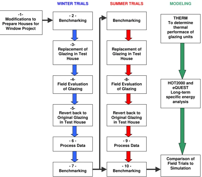
445H

Figure 1 provides an outline of the different tasks and the sequence followed during their implementation.

(17)

-1- Modifications to Prepare Houses for

Window Project 2 -Benchmarking -3-Replacement of Glazing in Test House -4-Field Evaluation of Glazing

WINTER TRIALS SUMMER TRIALS

-5-Revert back to Original Glazing in Test House 6 -Process Data Benchmarking Replacement of Glazing in Test House -8-Field Evaluation of Glazing Revert back to Original Glazing in Test House 7 -Benchmarking 9 -Process Data 10 -Benchmarking MODELING THERM To determine thermal performace of glazing units HOT2000 and eQUEST Long-term specific energy analysis Comparison of Field Trials to Simulation

Figure 1 - A schematic diagram showing the different tasks in the project Task 1: Preparing the test house for benchmarking:

The objective of this task is to modify the existing window frames so that window systems can be replaced with relative ease, allowing for a number of such experiments and others involving other technologies in rotation through a single season. The existing glazing units of both houses were identical. Their properties are given in Section 446H4.

The windows were converted to a dry glazing system with double sided glazing tapes and screw in place stops in order to facilitate the insulating glass (IG) units replacement. These changes were made without changes in the thermal properties of the windows or

(18)

Following these alterations, it was necessary to benchmark the two houses to ensure that performance remained unchanged, and to identify any variations in energy use. Task 2: Benchmarking of the Test House and Reference House after window modifications:

Following the installation of the modified windows, measurements were taken and data was collected over a one-week benchmarking period to confirm that the modifications to the window system had not altered the benchmark. During this period, the energy performance of the two houses was compared using the hard coat low emissivity glazing system that is originally installed in the houses. Further benchmarking periods occurred over the course of the heating season to ensure that the benchmark has not drifted, and to help develop the full benchmark across a range of outdoor conditions. This complete benchmark was also shared with other projects that heating season.

Task 3: Deglazing all windows and patio door in the Test House and installing replacement glazing with generic low solar heat gain coating on glass:

In this task, all glazing systems in the Test House were replaced by identical systems using generic low solar heat gain coating on glass.

Task 4: Field measurements of the low solar heat gain glazing during heating season:

Detailed monitoring of indoor and outdoor conditions, energy use in both houses, glass and frame surface temperatures was performed over a four week period during the heating season (19-Jan-06 to 15-Feb-06).

Task 5: Deglazing and replacement of IG units in Test House to its original configuration (high solar heat gain glazing):

Following completion of the monitoring of the Test House for the winter season, this task brings the Test House back to its original configuration by replacing all the IG units with the original units (high solar heat gain glazing).

Task 6: Processing of the data collected during the heating season:

For the four weeks total monitoring period during the heating season, all data and measurement were processed to determine the energy consumption and other parameters of interest during that period.

Task 7: Benchmarking the two houses after deglazing and replacement of IG units:

Following the replacement of the glazing units and reverting the Test House to its original configuration, the two houses were benchmarked to ensure that there were no changes to the baseline of energy use as a result of deglazing/replacement/reglazing tasks, as discussed above. Air leakage tests were also performed at this time to confirm the continuing air tightness of the houses.

(19)

Task 8: Field measurements of the low solar heat gain coated glass during cooling season:

Detailed monitoring of indoor and outdoor conditions, energy use in both houses, glass and frame surface temperatures were performed over four weeks period during the cooling season (July/August 2006), similar to Task 2 through 5 above.

Task 9: Processing of the data collected during the cooling season:

During the four weeks of monitoring of the two houses during the cooling season, all data and measurement were processed to determine the energy consumption and other parameters of interest during that period.

Task 10: Benchmarking the two houses after deglazing and replacement of IG units:

Following the replacement of the glazing units and reverting the Test House to its

original configuration, benchmarking the two houses was done to ensure that there were no changes to the baseline of energy use as a result of deglazing/replacement/reglazing tasks.

Task 11: Final report:

A final report was prepared to include the results of all the tasks from 1 to 10 above.

4

3B

Description of Glazing Technology

4.1

11B

Glazing Technology

High performance windows for residential glazing control undesirable heat gains and heat losses. In the colder northern half of North America, heat losses dominate and it is desirable to minimize heat loss and maximize solar gains to achieve satisfactory cold-climate performance. The heat transfer coefficient (U-Factor) of a single glazed window, 5.96 W/m2.K, can be reduced to 2.84 W/m2.K by double glazing (using clear glass) and further reduced to around 1.7 W/m2.K by tripling the glazing (clear glass) or by using a low emissivity coating with double glazing. Solar heat gains, while unwanted in summer, are beneficial in winter for heating purposes. Transparent low emissivity coatings are available in 3 types (all reflect invisible far infrared wavelengths and so all reduce

conductive window heat transfer): these 3 different low emissivity coating types transmit, reflect, or absorb (at different proportions) amounts of invisible near-IR solar energy, thus affecting the net solar heat gain of a residence. The Solar Heat Gain Coefficient (SHGC ) is a measure of this net solar heat gain. All 3 types of low emissivity coating are essentially visibly clear in appearance, transmitting over 55% of daylight when double-glazed, with negligible visible tint or reflectivity.

(20)

need to be protected from atmospheric moisture by enclosing them within a sealed double glazed unit.

CVD coatings are made with a hard low emissivity coating, pyrolytically applied to hot glass, at atmospheric pressure. They can be exposed to atmospheric humidity and water, and even single glazed with the coating exposed, if desired.

A residential designer’s dilemma is to select the most cost effective, thermally appropriate glazing, while still allowing high visible light transmission

4.2

12B

HSG and LSG Nominal Characteristic:

In the benchmark configuration, both the Test House and the Reference house at CCHT were glazed with high solar heat gain, CVD coated low emissivity, sealed double glazed units (nominal center of glass U-Factor = 1.65 W/m2°K (0.29 Btu/hr.ft2.°F), and nominal SHGC = 0.72).

In the experimental configuration, the Reference House was left in Benchmark condition (unchanged) and the Test house was re-glazed with a low solar heat gain, low

emissivity, sputter-coated low emissivity glass, (nominal center of glass U-Factor = 1.36 W/m2°K (0.24 Btu/hr.ft2.°F), and nominal SHGC = 0.41).

Figure 2 below illustrates the glazing systems and a sample of peak glass surface temperature during summer and winter seasons. For a full table of window properties, Refer to 447HTable 8.

WINTER

SUMMER 38°C 41°C 40°C 34°C

Reference House Test House

HSG LSG 11°C _45°C _18°C _33°C 1 2 3 4 1 2 3 4 Surface: -10°C 27°C Outdoor T

Figure 2 - Illustration of the glazing systems, with example peak window surface temperatures on clear days in summer and winter

(21)

4.3

13B

Measurement of Argon Concentration

The argon content of both the HSG and LSG windows was measured using a portable Sparklike Gasglass-1002 argon tester. In general, gas content of the newer LSG

windows was approximately 8% lower than the gas content of the HSG windows. Out of the 31 original HSG windows that were installed in 1998, the argon tester failed to make a reading on 5 of the windows. Argon gas content of the remaining 26 windows ranged from 68% to 98%, with an average of 92%. Argon content of the new LSG windows ranged from 70% to 97%, with an average gas content of 84%. These numbers were used in the simulation comparisons as described in Section 448H7. Detailed gas

(22)

5

4B

Field Monitoring:

5.1

14B

Approach

Field trials were conducted at the CCHT twin-house facility; refer to Section 450H5.2 for a full

description of the facility.

For both winter and summer testing, periods of benchmarking were conducted before and after the experiment. During benchmarking, the houses are maintained in identical configuration, with the HSG windows installed in both. The purpose of this

benchmarking was twofold: to determine the existing differences between the houses, and to ensure that no changes in house energy consumption occurred as a result of the window experiment.

5.2

15B

CCHT Twin House Facility

Built in 1998, the Canadian Centre for Housing Technology (CCHT) (218H

www.ccht-cctr.gc.ca) is jointly operated by National Research Council (NRC), Natural Resources

Canada (NRCan), and Canada Mortgage and Housing Corporation (CMHC). CCHT’s mission is to accelerate the development of new technologies and their acceptance in the marketplace.

Figure 3 - CCHT Twin-House Facility - Control House (left) and Experimental House (right)

The Canadian Centre for Housing Technology features twin research houses to evaluate the whole-house performance of new technologies in side-by-side testing. See 451HFigure 3,

which shows the Control and the Experimental houses. These houses were designed and built by a local builder to the R-2000 standard. The houses are a popular model

(23)

currently on the market in the region, and were built with the same crews and techniques normally used by the builder. A full list of the twin houses characteristics can be found in

452H

Table 1.

Table 1 - Twin House Characteristics

Feature Details

Construction Standard R-2000

Liveable Area 210 m2 (2260 ft2), 2 storeys

Insulation Attic: RSI 8.6, Walls: RSI 3.5, Rim joists: RSI 3.5 Basement Poured concrete, full basement

Floor: Concrete slab, no insulation

Walls: RSI 3.5 in a framed wall. No vapour barrier.

Garage Two-car, recessed into the floor plan; isolated control room in the garage

Exposed floor over the garage RSI 4.4 with heated/cooled plenum air space between insulation and sub-floor.

Windows Area: 35.0 m2 (377 ft2) total, 16.2 m2 (174 ft2) South Facing Double glazed, high solar heat gain coating on surface 3. Insulated spacer, argon filled, with argon concentration measured to 95%.

Air Barrier System Exterior, taped fiberboard sheathing with laminated weather resistant barrier. Taped penetrations, including windows. Airtightness 1.5 air changes per hour @ 50 Pa (1.0 lb/ft2)

Furnishing Unfurnished

The CCHT twin houses are fully instrumented and are unoccupied. To simulate the normal internal heat gains of lived-in houses, these houses feature identical ‘simulated occupancies’. The simulated occupancy strategy is described in 453HAppendix A.

The house’s mechanical systems consisted of a 94% efficiency condensing gas furnace to provide heating, and a 2 ton 12 SEER air conditioning unit to provide cooling.

Additional details of the configuration and mechanical systems are listed in 454HTable 2.

Table 2 Operating Conditions for the Standard CCHT Benchmark

System Control House Experimental House

1a Furnace

High efficiency condensing gas furnace; continuous circulation, 94% steady state efficiency (measured)

1b Air Conditioner 2 ton, 13 SEER system 2 ton, 13 SEER system

2 Thermostat

A single centrally located thermostat, set point: 22°C (72 °F) winter 26°C (79 °F) summer

(24)

4 Interior Doors All interior doors open All interior doors open

5 Window Exterior Shades

No shades on the west-facing diamond shaped window, or the south-facing bedroom window containing the pyranometer All other interior blinds down with slats in the horizontal position

No shades on the west-facing diamond shaped window, or the south-facing bedroom window containing the pyranometer All other interior blinds down with slats in the horizontal position 6 Windows Closed, Airtightness ~1.5 ach Closed, Airtightness ~1.5 ach 7 Simulated

Occupancy Standard Schedule Standard Schedule

8 Humidifier Off Off

9 Hot Water Heater Standard Gas, 67% efficiency (measured)

Standard Gas, 67% efficiency (measured)

10 Thermostat

Programmable thermostat, Standard central location on first floor

(25)

5.3

16B

Window Installation

The windows were converted to a dry glazing system (not requiring a wet sealant or glazing compound) using double sided glazing tapes and screw in place stops in order to facilitate the insulating glass (IG) units replacement.

The Test House contains one set of patio doors and three different types of windows: operable casement, fixed casement, and fixed windows. The procedure for replacing the HSG glazing units with LSG glazing units was unique for each type of window. See

455H

Appendix C for photos of the replacement process.

Operable casement windows

For operable casement windows, identical window sashes and hinge hardware were acquired. The original window and sash were then removed from the hinges, and the replacement window with sash were secured in place.

Non-Operable casement windows

For non-operable casement windows, the screws holding the window sash to the window frame were broken to facilitate replacement. The glazing unit complete with sash was then removed from the frame, a replacement window and sash was put in its place. The replacement window was then secured by means of 6 easily accessible screws, fastened through the interior side of the sash into the window frame. Although the windows in the Reference House were never replaced, the modifications to the fasteners were completed to help to maintain the similarities between the two houses, and also as a facility upgrade to enable the windows of both houses to be changed for future experiments.

Fixed windows

The original fixed windows were held in place using a wet seal. Caulking was removed from the joint between the window and trim on the exterior and interior of the window. The interior trim was removed from the periphery of the window. The wet seal was cut and the glazing unit removed. The replacement glazing unit was sealed using a two-sided glazing tape. The trim was reinstalled and a bead caulking was applied to the exterior and interior perimeter of the window.

Patio doors

The replacement glazing units were installed in a set of patio door casements. The original doors were removed, and the new doors were installed in their place.

(26)

5.4

17B

Monitoring Protocol and Parameters

During winter testing, summer testing, and benchmarking alike, a number of parameters were monitored:

5.4.1 31BSolar Radiation

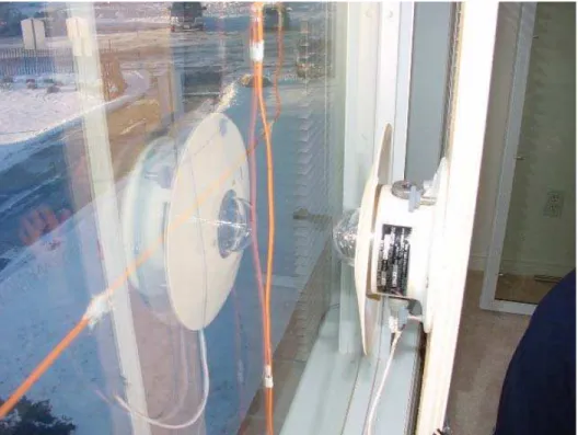
A precision spectral pyranometer mounted on the south-facing brick wall of the

Reference House measured total global solar radiation on the vertical plane. A second identical pyranometer was mounted behind the south-facing window of the Test House bedroom 2. The difference between the readings of the two pyranometers was used as an indication of the transmission properties of the window. The pyranometers’

measurements cannot be seen as an absolute measurement of transmission, as the field of view of the window-mounted pyranometer is obstructed partially by the surrounding window frame (see 456HFigure 4). However, this measurement was used to

compare the two sets of windows – during benchmarking, and during the experiment. Pyranometer measurements, in W/m2, were recorded on a 5-minute basis and daily totals, in kJ/m2/day, were calculated for the analysis.

Figure 4 - Precision Spectral Pyranometer mounted in the Test House south-facing bedroom window

5.4.2 32BFurnace Consumption

In each house, an electric meter with pulse output measured the furnace circulation fan electricity consumption and a gas meter with pulse output measured the furnace natural gas consumption. Measurements were recorded on a 5-minute basis, at a resolution of 0.0006 kWh/pulse, and 0.05 ft3/pulse respectively. Daily totals for both electrical and gas consumption were used in the analysis.

(27)

5.4.3 33BWindow Surface Temperatures

Window surface temperatures were monitored at one exterior and three interior locations on each window (see 457HFigure 5) by thermocouples mounted to the window surface using

a thermally conductive epoxy. The accuracy of temperature measurements was +/- 0.1°C. A total of five windows were instrumented – two on the south face of the building, and one window on each of the north, east, and west faces. 458HFigure 6 shows photos of

all four faces of the research house. Instrumented windows are circled.

Center of Glass Edge of Glass Edge of Glass Interior Exterior 2.5 cm (1 in.) 2.5 cm (1 in.)

Figure 5 - Window Thermocouple locations

(28)

5.4.4 34BAirtightness testing

A standard blower door test was performed prior to and following the window experiment in both summer and winter, using the procedure outlined in CAN/CGSB-149.10 – M86, A

Method for Testing the Airtightness of Buildings by the Fan Depressurization Method.

This was done to verify that the houses maintained their airtightness despite changes to the envelope (window replacement).

5.4.5 35BSouth-facing Room Temperatures

Room air temperatures were recorded hourly in each of the four south-facing rooms: livingroom, bedroom 2, master bedroom and ensuite, at three different heights: ceiling level, mid height and floor level. The accuracy of temperature measurements was +/- 0.1°C. Refer to 459HAppendix H for floor plans of the Research Houses, including supply

(29)

5.5

18B

Winter Results

5.5.1 36BWeather

The winter comparison of the HSG and LSH glazing units performance was conducted for a four-week period from January 19th to February 15th, 2006. The outdoor

temperature and solar conditions during that period are shown in 460HFigure 7 and 461HFigure 8.

During the monitoring period, outdoor temperature ranged from –18.6°C to 7.54°C. Daily solar radiation incident on the south face of the house ranged from 1205 kJ/m2/day to 22599 kJ/m2/day.

Outdoor Temperature during Winter Window Glazing Experiment

-20 -15 -10 -5 0 5 10

19-Jan-06 0:00 23-Jan-06 0:00 27-Jan-06 0:00 31-Jan-06 0:00 04-Feb-06 0:00 08-Feb-06 0:00 12-Feb-06 0:00 16-Feb-06 0:00 Date an d Time O u tdo or Te m pe ra tur e ( °C ) Outdoor Temperature

Figure 7 - Range of Outdoor Temperatures during Winter

Solar Radiation during Winter Window Glazing Experiment

200 400 600 800 1000 1200 a d iat io n i n ci d e n t o n a ver ti ca l s o u th -f ac in g s u rf ac e, W /m 2 Vertical Solar

(30)

5.5.2 37BWinter Benchmarking

Benchmarking occurred before and following the winter test period. In total, 13 days of data were collected in benchmarking configuration prior to the window experiment, and 10 days of data were collected following the experiment. The days spanned the winter season between 29-Oct-05 and 12-Mar-06. Temperature readings during the

benchmarking days ranged from -18.9°C to 15.9°C. Total daily vertical solar radiation on the south face ranged from 871 kJ/(m2._{day) to 21905 kJ/(m}2._day).

Furnace gas consumption data from benchmarking before and after the experiment is plotted in 462HFigure 9. Total daily Reference House furnace gas consumption is plotted on

the x-axis, while total daily Test House furnace gas consumption is plotted on the y-axis. Each point represents a single day of data. By plotting multiple days, a trend can be developed to indicate the relative performance of the two houses. If the two houses were in fact perfectly identical, the benchmark would have a slope of 1 and intercept at 0. There are always small differences between the houses, as it is impossible for them to be completely identical. This is seen by the slightly higher slope, and intercept that is less than 1 in both trends.

The “before” and “after” trends in this graph are very similar. Along the length of the trend lines, they stay within 7 MJ of one another. Experimental scatter could easily account for these small differences. The similarity in the trend lines indicates that the performance of the houses remained unchanged in terms of energy consumption by the window experiment. Additionally, this similarity allows all benchmarking data to be considered as a single trend. For the remainder of the winter analysis section, winter benchmarking data will appear as a set of data, and will not be split into two separate trends.

Furnace Natural Gas Consumption

y = 1.0175x - 1.7899 R2_{= 0.998} y = 1.0508x - 12.317 R2_{= 0.9954} 0 100 200 300 400 500 600 0 100 200 300 400 500 600

Reference House Furnace Natural Gas Consumption (MJ/day) T e s t H ou s e Fu rna c e N a tu ra l G a s C o ns ump ti o n ( M J /d a y )

Benchmarking Before Glazing Experiment

Benchmarking After Glazing Experiment

Linear (Benchmarking Before Glazing Experiment) Linear (Benchmarking After Glazing Experiment)

Benchmark before Experiment

Benchmark after Experiment

Figure 9 - Winter Benchmarking Furnace Gas Consumption Curve before and after the experiment.

(31)

5.5.3 38BFurnace Natural Gas and Electrical Consumption

During the experiment, furnace natural gas consumption was monitored in both houses. The resulting daily consumption data is plotted along side the benchmarking data in

463H

Figure 10. On average, the results show an increase in gas consumption due to the installation of the LSG windows. The average increase over the duration of the winter monitoring period was 23 MJ/day, with a maximum increase of 60 MJ/day.

Furnace blower fan electrical consumption data during the experiment and benchmark are plotted in 464HFigure 11. On average, the results show an increase in blower electrical

consumption due to the installation of the LSG windows. The average increase over the duration of the winter monitoring period was 0.13 kWh/day, with a maximum increase of 0.48 kWh/day.

Over the entire experimental period in the winter, the simple addition of increased consumption associated with the LSG technology was 8.7% for gas and 1.3% for electricity.

The large amount of scatter in the glazing experiment data can be related directly to solar radiation. On days with high amount of solar radiation, the differences between the windows have greater impact, and the data point is further away from the benchmark trend line. On days with low amounts of solar radiation, points are much closer to the benchmark trend, and on a few occasions are below the benchmark line. The

relationship between solar radiation and consumption data is further discussed in next section.

(32)

Furnace Natural Gas Consumption y = 1.0217x - 3.8078 R2_{= 0.9971} 0 100 200 300 400 500 600 0 100 200 300 400 500 600

Reference House Furnace Natural Gas Consumption (MJ/day)

Te s t H ous e Fu rna c e N a tu ra l G a s C o n s u m pt io n ( M J /d a y ) Benchmarking 2005-2006 no shades

Window Glazing Project Linear (Benchmarking 2005-2006 no shades )

Benchmark 2005-2006

Figure 10 - Winter Furnace Gas Consumption

Furnace Electrical Consumption

y = 0.9953x + 0.025 R2_{= 0.9907} 7 8 9 10 11 12 13 7 8 9 10 11 12 13

Reference House Furnace Electrical Consumption (kWh/day)

Test House Furnace Electri

cal Consumption (kWh/day)

Benchmarking 2005-2006 - no shades Window Glazing Project

Linear (Benchmarking 2005-2006 - no shades)

Benchmark 2005-2006

(33)

5.5.4 39BSolar Transmission

The most notable difference between the windows is their ability to transmit solar radiation. This difference is demonstrated in 465HFigure 12. Two days of solar data are

plotted in this graph: January 15th_{– a Benchmark day, and January 26}th_{– an Experiment} day. On January 15th_{, a pyranometer was mounted behind a south-facing HSG window.} On January 26th_{, the pyranometer was situated at the same south-facing location,}

behind a low solar heat gain low emissivity (LSG) window. Only 40% of the total solar radiation incident on a wall with the same orientation as the window was detected behind the LSG window. Whereas, 60% of the solar radiation was transmitted by the high solar heat gain low emissivity (HSG) window. (These numbers do not include the energy absorbed, convected and radiated to the room – factors included in the SHGC. Measured window temperatures discussed below give an indication of those effects). A relationship can be drawn between total daily solar radiation incident on the south facing wall of the House, and total transmitted solar radiation (as captured by the pyranometer mounted behind the window). This relationship is presented in 466HFigure 13

for both the HSG and LSG windows. The slope of these lines gives a quick

approximation of the percentage of solar radiation being detected in the room. For the HSG windows, the slope is approximately 0.59, and the slope of the LSG curve is approximately 0.40.

An alternative representation of these relationships is plotted in 467HFigure 14. The

percentage of solar radiation transmitted by the window is plotted against the total solar radiation incident on the south face of the house. Again, the curves indicate that on average 40% of the incident solar radiation is reaching the room side of the LSG window, while 57% on average was detected behind the HSG window. On days with low solar gains, where less than 4000 kJ/m2/day were incident on the south face of the house, the relationship between percentage of transmitted solar energy and total solar energy breaks down. On these days, the percentage of solar energy transmitted by the windows dropped for both the LSG and HSG windows. This result demonstrates that on days with low solar gains, generally very cloudy days, the spectrally selective properties of the low emissivity coating associated with the two different technologies are of less importance.

(34)

Transmitted Solar Energy, Winter

0 200 400 600 800 1000 1200 0: 00 2: 00 4: 00 6: 00 8: 0 0 10: 00 12: 00 14: 00 16: 00 18 :0 0 20: 00 22 :00 _0:00 _2:00 _4:00 _6:00 _8:00 10: 00 12: 00 14 :0 0 16: 00 18 :00 20: 00 22: 00 Time, hh:mm Sol a r En e rgy , W/ m 2 0 63 127 190 254 317 380 So la r E n er gy , B tu /( h .ft 2)

Pyranometer mounted vertically on South facing brick wall

Pyranometer mounted vertically behind HIGH SOLAR GAIN window

Pyranometer mounted vertically behind LOW SOLAR GAIN window

Total: 11604 kJ/m2_/day, ~60% Total: 8327 kJ/m2_/day, ~40% Total: 19239 kJ/m2_/day Total: 20643 kJ/m2_/day Peak: 581 W/m2 Peak: 407 W/m2 HSG LSG 15-Jan-06 26-Jan-06

Figure 12 - Transmitted Solar Energy during Winter Glazing Experiment

Window Transmission of Solar Radiation

y = 0.5936x - 181.81 R2 = 0.9952 y = 0.4012x - 23.079 R2_{= 0.9979} 0 2000 4000 6000 8000 10000 12000 14000 0 5000 10000 15000 20000 25000

Total Daily Solar Radiation on Incident on South Face of Reference House (kJ/m2)

D a il y S o la r R a di a ti on c a pt ur e d be hi nd w indo w ( k J /m2 )

High Solar Gain on Surface 3 Low Solar Gain on Surface 2 Linear (High Solar Gain on Surface 3) Linear (Low Solar Gain on Surface 2)

Figure 13 - Daily Solar Radiation Measured in the room as a function of Daily Solar Radiation Measured at the South Face of the Houses

(35)

Percentage of Incident Radiation captured by Pyranometer behind CCHT Test House Window (Existing Windows)

y = 1E-06x + 0.5677 y = -6E-08x + 0.4014 0% 10% 20% 30% 40% 50% 60% 70% 0 5000 10000 15000 20000 25000

Total Da ily S olar Radiation on Incident on South Fac e of Referenc e House ( kJ/m2)

D a il y S o la r R a di a ti o n c a p tu re d be hi n d w ind o w ( a s a pe rc e n ta g e of s o la r ra d ia ti on i n c ide nt o n S o ut h Fa c e )

HSG glass - Low radiation day (<4000)

HSG glass - High radiation day (>4000) LSG glass - Low radiation day (<4000)

LSG glass - High radiation day (>4000) Linear (HSG glass - High radiation day (>4000))

Linear (LSG glass - High radiation day (>4000))

Figure 14 - Daily Solar Radiation Measured as a Percentage of Daily Solar Radiation Measured at the South Face of the Houses

(36)

5.5.5 40BCausal Relationships Between Solar Transmission and Heating Energy

Consumption

With the LSG windows transmitting less solar energy, the heating system has to

compensate for the loss. In 468HFigure 15, the change in gas consumption due to the LSG

windows is plotted against the daily solar radiation incident on the south facing wall of the house. Change in gas consumption is equivalent to the vertical distance between the data point and the benchmark correlation line in 469HFigure 10. The gas consumption VS

total solar radiation correlation is strong, with an R-squared value of 0.94. The increase in consumption due to the LSG windows is highest on the days with the largest solar gains. Thus, on the sunniest days, the house with the LSG windows is not receiving the same benefit from solar gains as the house with HSG windows, and has to compensate by consuming more gas for heating.

Increase in Gas Consumption VS Total Vertical Solar Radiation

y = -1E-07x2 + 0.0058x - 14.389 R2 = 0.9449 -20 -10 0 10 20 30 40 50 60 70 0 5000 10000 15000 20000 25000

Total Solar Radiation Incident on South -facing wall (kJ/m2/day)

D if fe ren ce i n F u rn a ce G a s C o n su m p ti o n f ro m B en ch m a rk ( M J /d ay)

warm sunny days, 28-Jan and 1-Feb Ref house thermostat T > Test house thermostat T

Figure 15 - Relationship between Gas Consumption and Total Incident Daily Vertical Solar Radiation

The same relationship can be expressed directly in terms of reduction in solar gains due to the use of the LSG windows, and the resulting increase in furnace gas consumption, see 470HFigure 16. This graph highlights the tradeoff between lost solar gains and

increased heating system operation. On the sunniest days, the house with the LSG windows had to compensate for the lost solar gains by consuming more than 50 MJ more natural gas.

The trend on this graph intercepts the y-axis below zero, indicating that there are some differences of the thermal performance of the two types of windows. On days with very low solar gains, the LSG windows appear to be slightly outperforming the HSG windows.

(37)

The window surface temperatures provide other evidence of this phenomenon (refer to Section 471H5.5.6 for further discussion).

The two data points that do not fall on the curve in 472HFigure 16 (i.e., outliers) are a result of

outdoor conditions. On these two days, hot temperatures and high solar gains caused the Reference House temperatures to drift above the control of the thermostat. The 22-degree thermostat setting maintains the house between approximately 20.5°C and 22.5°C. On the day presented in 473HFigure 17, the Reference House temperature

exceeded the thermostat deadband for more than 5 hours during the middle of the day. The same was not true for the Test House, fitted with the LSG windows. Without the added solar gains, the Test house temperature attained the top of the thermostat deadband, but did not exceed it.

Relationship between Increase in Furnace Consumption and Decrease in Transmitted Solar Radiation

y = -3E-06x2 + 0.0284x - 10.181 R2 = 0.9368 -20 -10 0 10 20 30 40 50 60 70 0 500 1000 1500 2000 2500 3000 3500 4000 4500 5000

Decrease in Solar Radiation Entering through window from Benchmark condition (kJ/m2/day)

In cr e ase i n F u rn ac e G a s C o n s u m p ti o n f ro m B en c h m ar k (M J /d a y )

warm sunny days, 28-Jan and 1-Feb Ref house thermostat T > T est house thermostat T

Figure 16 - Relationship between Increase in Furnace Gas Consumption and Decrease in Transmitted Solar Radiation

(38)

CCHT Research Houses Main Floor Temperature 10 12 14 16 18 20 22 24 26 28 30 0:00 4:00 8:00 12:00 16:00 20:00 0:00 Time T em p er at u re ( °C ) Reference House Test House 28-Jan-06

Thermostat dead band

(39)

5.5.6 41BNight Time Analysis

An analysis of night time gas consumption (from 10 p.m. to 6 a.m.) was conducted to determine whether there were any significant differences in the thermal performance of the two window technologies under investigation. The experiment and benchmark results are plotted in 474HFigure 18. Some evidence of thermal differences was detected in

the increase in furnace gas consumption VS solar radiation curves, as discussed in the previous section. Window surface temperatures also confirmed a slight difference in window thermal performance (475HFigure 19). Over night, the exterior window surface of the

LSG window dropped ~1°C below the temperature of it’s twin HSG window in the Reference House. On the interior pane, the opposite was true. The interior surface of the LSG window was slightly warmer than the surface of the HSG window. These temperatures indicate that more heat is escaping through the HSG window than the LSG window. However, the analysis of gas consumption over night – when no solar gains would affect the results – revealed that these small differences resulted in no significant change in gas consumption. Thus, differences in solar performance, and not thermal performance, were the main cause of the change in heating load caused by the windows.

Furnace Natural Gas Consumption 10 p.m. to 6 a.m.

y = 1.0489x - 2.7207 R2_{= 0.9951} y = 1.092x - 11.649 R2 = 0.9789 0 50 100 150 200 250 300 0 50 100 150 200 250 300

Reference House Furnace Natural Gas Consumption (MJ/night) T e s t H o u s e F u rn a c e N a tu ra l G a s C o ns u m pt io n (M J /n ig h t) Benchmarking 2005-2006 no shades

Window Glazing Project

Linear (Benchmarking 2005-2006 no shades )

Linear (Window Glazing Project)

Benchmark 2005-2006

Window Glazing Project

(40)

Window Surface Temperatures - Bedroom 2 (South) -15 -10 -5 0 5 10 15 20 25 30 35 40 45 50 0:00 2:00 4:00 6:00 8:00 10:00 12:00 14:00 16:00 18:00 20:00 22:00 0:00 Time T em p er a tu re ( °C )

Reference House Centre Ext. Test House Centre Ext. Reference House Centre Int. Test House Centre Int.

26-Jan-06

At night, the interior surface of the Test House Window (Low Solar Gain on S2) is ~1°C warmer than the Reference House Window

The opposite is true on the exterior surface

Figure 19 - South-facing Window Surface Temperatures

5.5.7 42BWindow Temperatures

During the benchmarking period, the two sets of HSG windows performed similarly in terms of window surface temperatures. 476HFigure 20 shows temperature data at the centre

of the glass for a single sunny day during benchmarking. This graph demonstrates that both the interior temperature and exterior pane temperatures track closely. The

difference between the curves from 8:30 to 10:00 is caused by a building shadowing one house and not the other. This phenomenon occurs in late December and early January, when the sun is low in the sky. The effect of this shadow on consumption is taken into account in the side-by-side analysis method and benchmark. The maximum

temperature attained at the centre of the interior pane, and at the centre of the exterior pane can be plotted on a daily basis, as shown in 477HFigure 21. The maximum daily

Reference House window temperature is plotted on the x-axis, while the maximum daily Test House temperature is plotted on the y-axis. Trend lines are developed for both the interior and exterior surface temperatures. Were the houses and windows completely identical, these trend lines were have a slope of 1 and intercept 0. In reality, the trend lines come very close to this ideal – demonstrating the similarity between the two sets of HSG windows.

(41)

Window Surface Temperatures - Living Room (South) -20 -15 -10 -5 0 5 10 15 20 25 30 35 40 45 50 0:00 2:00 4:00 6:00 8:00 10:00 12:00 14:00 16:00 18:00 20:00 22:00 0:00 Time T em p er a tu re ( °C )

Reference House Centre Ext. Test House Centre Ext.

Reference House Centre Int.

Test House Centre Int. 15-Jan-06

Maximum Interior surface temperature

Maximum Exterior surface temperature

Figure 20 - South facing window surface temperature during benchmarking

Livingroom - South Facing Window

y = 1.0234x + 0.0467 R2_{= 0.9984} y = 1.067x - 1.3955 R2 = 0.9994 -20 -10 0 10 20 30 40 50 -20 -10 0 10 20 30 40 50 Te s t H ous e D a il y M a x im u m T e m pe ra tu re a t C e ntr e o f W indo w ( °C

) Living room Benchmark - Exterior

Living room Benchmark - Interior

Linear (Living room Benchmark -Exterior)

Linear (Living room Benchmark -Interior) Exterior Pane Interior Pane Maximum Daily Interior surface temperature Maximum Daily Exterior surface temperature