Application of multiple model control to space structure systems with nonlinear inertial properties

Application of Multiple Model Control to

Space Structure Systems with

Nonlinear Inertia Properties

by

Kazumi Masuda

Submitted to the Department of Aeronautics and Astronautics in partial fulfillment of the requirements for the degree of

Master of Science in Aeronautics and Astronautics at the

MASSACHUSETTS INSTITUTE OF TECHNOLOGY

June 1995

@

Author.. ...

Department of Aeronautics and Astronautics May 22, 1995

A

Certified by ... ... ...

Dr. David W. Miller Principal Research Scientist, Department of Aeronautics and Astronautics Thesis Supervisor

A ccepted by ... ... .... ... ...

Professor Harold Y. Wachman Chairman, Department Graduate Committee

MASSACHUSETTS INSTITUTE OF Tprttrwmi nrw

'JUL 07 1995

LIBRARIES

Application of Multiple Model Control to

Space Structure Systems with

Nonlinear Inertia Properties

by

Kazumi Masuda

Submitted to the Department of Aeronautics and Astronautics on May 22, 1995, in partial fulfillment of the

requirements for the degree of

Master of Science in Aeronautics and Astronautics

Abstract

Future space systems will require high robustness of the control system as well as high performance because of their two major features: lightly damped structural dy-namics; and nonlinear inertia properties induced by the large motion of articulating sensor heads and antennas. Effective robust control design techniques are needed to satisfy the performance requirements of future space systems in the presence of model uncertainties and nonlinear changes in their inertia properties.

In this thesis, the Multiple Model (MM) technique is applied to a plant system which has multiple off-nominal factors including nonlinear inertia properties. Three control design problems are presented to examine the effectiveness of the MM tech-nique: sample designs for a simple plant system; single-input, single-output (SISO) designs for the Middeck Active Control Experiment (MACE); and multiple-input, multiple-output (MIMO) designs for the MACE. A plant model of the MACE test article has two off-nominal factors, i.e. frequency uncertainty in the Z-axis bending modes and nonlinear inertia changes due to different primary payload average angles. In each design problem, LQG compensators are first designed and used as initial com-pensators in the subsequent MM designs. Through the comparison between LQG and MM compensators, the effectiveness of the MM technique is examined.

In every design problem, the MM technique enhances robust stability and perfor-mance of an original LQG compensator with small loss in nominal perforperfor-mance. In particular, in the MIMO designs for the MACE, the MM technique substantially im-proves robust performance for nonlinear inertia properties of the MACE test article. This research reveals the effectiveness of the MM technique for multiple off-nominal factors including nonlinear changes of inertia properties.

Thesis Supervisor: Dr. David W. Miller

Title: Principal Research Scientist, Department of Aeronautics and Astronautics

Acknowledgments

I would like to thank my advisor, Dr. David Miller, for his guidance and support through the course of my research.

I would also like to thank the members of the MACE team for their suggestions and encouragement. Simon Grocott gave me technical advice on numerous occasions. Roger Glaese provided me with design data for a plant model. Mark Campbell gave me valuable suggestions. Without their support, this thesis would not have been completed within the limited time.

Special appreciation goes to Professor Wallace E. Vander Velde, who guided me from the start of my study at MIT and introduced me to this exciting MACE pro-gram.

Additional thanks goes to Professor Richard H. Battin, who greatly influenced me not only through his lectures of Astrodynamics at MIT but also through his outstanding contribution in the Apollo project.

Special appreciation goes to Dr. Paul E. Brown, Director of the Advanced Study Programs at MIT, who introduced me to MIT and gave me valuable encouragement and support.

Finally, I would like to thank Mitsubishi Heavy Industries, Ltd. for the opportu-nity to study at MIT.

Contents

1 Introduction

1.1 Robust Control Design techniques . . . . 1.2 Middeck Active Control Experiment (MACE) . . 1.3 Motivation, Objectives, and Outline . . . .

2 Control Design Techniques and Sample Designs

2.1 Linear Quadratic Gaussian (LQG) . . . .

2.1.1 Formulation ... 2.1.2 Design Strategy ...

2.2 Multiple Model (MM) Method . . . . 2.2.1 Formulation ...

2.2.2 Design Strategy . . . . 2.3 Sample Designs ...

2.3.1 Plant System for the Sample Designs . . 2.3.2 Analysis Tools ... 2.3.3 LQG Designs ... 2.3.4 MM Designs ... 2.4 Conclusions ... 17 17 25 25 26 31 35 35 38 40 40 49 53 65 75

3 SISO Control Designs for the 4-Mode Flexible MACE Model 77

3.1 SISO Plant System ... 78

3.1.1 M odeling . . . . 78 3.1.2 Nonlinear Inertia Property Effects ... . 83

7

3.2 LQG Designs ... ... ... .. 87

3.3 MM Designs ... 99

3.3.1 FU-MM compensator ... ... ... .... . 102

3.3.2 FU&PG-MM compensator ... 108

3.4 Conclusions . . . 114

4 MIMO Control Designs for the 4-Mode Flexible MACE Model 119 4.1 MIMO Problem ... ... . 120

4.1.1 MIMO Plant System ... .... ... 120

4.1.2 Design Strategy ... ... .... . 124

4.2 LQG Designs ... ... .... ... .. 126

4.3 MM Designs ... ... . . ... 138

4.3.1 Low Authority MM Compensators ... .... ... 140

4.3.2 High Authority MM Compensators ... 147

4.4 Conclusions . ... ... 157

5 Conclusions ₁₅₉

A Derivatives of the Weighted Sum of the LQG costs in the MM

Method 163

List of Figures

1-1 Middeck Active Control Experiment (MACE) test article (ground

ex-periment configuration in l1-g) ... 20

2-1 General control system ... 27

2-2 Sample model; 4-mode free-free flexible beam . ... 41

2-3 Bode plot of the 4-mode free-free flexible beam ... 48

2-4 Pole-zero location of the 4-mode free-free flexible beam ... 48

2-5 Example of the LQG cost plot ... 50

2-6 Frequency responses of the LQG compensators and the plant system; 4-mode free-free flexible beam ... 54

2-7 Pole-zero location of the plant system and the LQG compensators . . 55

2-8 Pole-zero location of the closed loop systems with the LQG compensators 56 2-9 Frequency responses of the sensitivity transfer functions and compli-mentary transfer functions of the LQG compensators . ... 57

2-10 Performance of the LQG compensators . ... 58

2-11 Bode plots of the loop transfer functions of the LQG compensators 59 2-12 Bode plots of the loop transfer functions of the low authority LQG compensator and the plant systems disturbed in the second mode fre-quency . . . .. .. . 61

2-13 Pole-zero location of the low authority LQG compensator and the plant systems disturbed in the second mode frequency . ... 61

2-14 Bode plots of the loop transfer functions of the high authority LQG compensator and the plant systems disturbed in the second mode fre-quency ... . . . . .... . .. . . . . . . . .. 62 2-15 Pole-zero location of the high authority LQG compensator and the

plant systems disturbed in the second mode frequency ... 62 2-16 Nichols plots of the control system with the low authority LQG

com-pensator and high authority LQG comcom-pensator . ... 63

2-17 LQG costs of the closed loop systems with the LQG compensators . . 64

2-18 Performance of the low authority MM compensator ... . . 66 2-19 Performance of the high authority MM compensator ... . 67 2-20 Pole-zero location of the plant system and the low authority MM

com-pensators . ... .. ... ... ... . 68 2-21 Pole-zero location of the plant system and the high authority MM

com pensators . . . . .. . . . . . .. . . . . 69 2-22 Bode plots of the low authority MM compensator . ... 71 2-23 Bode plots of the high authority MM compensator . ... 71 2-24 Bode plots of the loop transfer functions of the low authority MM

com-pensator and the plant systems disturbed in the second mode frequency 72 2-25 Pole-zero location of the low authority MM compensator and the plant

systems disturbed in the second mode frequency ... . . . . 72 2-26 Bode plots of the loop transfer functions of the high authority MM

compensator and the plant systems disturbed in the second mode fre-quency ... .... . ... ... ... 73 2-27 Pole-zero location of the high authority MM compensator and the plant

systems disturbed in the second mode frequency ... . . . . 73 2-28 LQG costs of the closed loop systems with the low authority MM

compensator ... ... 74

2-29 LQG costs of the closed loop systems with the high authority MM

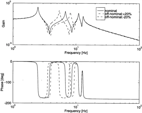
3-1 4-mode flexible MACE model ... 79 3-2 Bode plot of the 4-mode flexible MACE model with the frequency

uncertainty changes in the second Z-bending mode . ... 85 3-3 Pole-zero location of the 4-mode flexible MACE model with the

fre-quency uncertainty changes in the second Z-bending mode ... 85 3-4 Bode plot of the 4-mode flexible MACE model with the primary gimbal

angle changes . .. . . . .. . . . .. . 86 3-5 Pole-zero location of the 4-mode flexible MACE model with the

pri-mary gimbal angle changes ... 86 3-6 Pole-zero location of the LQG compensators and the nominal plant

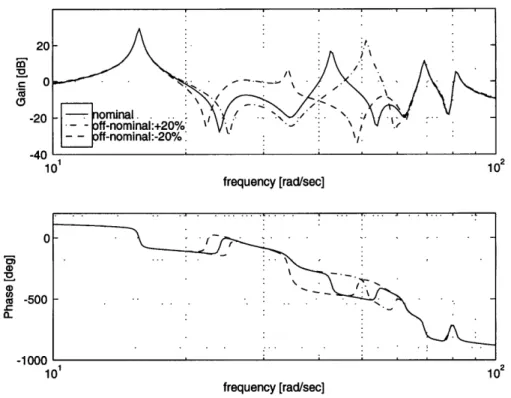
system . . . .. .. . 88 3-7 Frequency responses of the LQG compensators and the plant system. 89 3-8 Performance of the LQG compensators . ... 90 3-9 Comparison of LQG costs of the LQG compensators ... 92 3-10 Bode plots of the loop transfer functions of the low authority LQG

compensator and the plant system disturbed in the second mode fre-quency . . . .. .. . 93 3-11 Pole-zero location of the low authority LQG compensator and the plant

system disturbed in the second mode frequency . ... 93 3-12 Bode plots of the loop transfer functions of the low authority LQG

compensator and the plant system disturbed by the primary gimbal average angle . . . .. . . . .. . 94 3-13 Pole-zero location of the low authority LQG compensator and the plant

system disturbed by the primary gimbal average angle . ... 94 3-14 Bode plots of the loop transfer functions of the high authority LQG

compensator and the plant system disturbed in the second mode fre-quency . . . .. .. . 95 3-15 Pole-zero location of the high authority LQG compensator and the

plant system disturbed in the second mode frequency . ... 95

3-16 Bode plots of the loop transfer functions of the high authority LQG compensator and the plant system disturbed by the primary gimbal average angle ... .... 96 3-17 Pole-zero location of the high authority LQG compensator and the

plant system disturbed by the primary gimbal average angle .... . 96 3-18 LQG cost of the closed loop system with the low authority LQG

com-pensator ... ₉₇

3-19 LQG cost of the closed loop system with the high authority LQG com-pensator .. . ... . . . .. . . ... ... . . . . 98 3-20 Pole-zero location of the MM compensators and the nominal plant system 100 3-21 Frequency responses of the FU-MM compensator and the plant system 104 3-22 Performance of the FU-MM compensator . ... . . . . 104 3-23 Bode plots of the loop transfer functions of the FU-MM compensator

and the plant system disturbed in the second mode frequency . . .. 105 3-24 Pole-zero location of the FU-MM compensator and the plant system

disturbed in the second mode frequency ... . .. . . . . . 105 3-25 Bode plots of the loop transfer functions of the FU-MM compensator

and the plant system disturbed by the primary gimbal average angle. 106 3-26 Pole-zero location of the FU-MM compensator and the plant system

disturbed by the primary gimbal average angle ... . . . . 106 3-27 LQG cost of the closed loop system with the FU-MM compensator . 107 3-28 Frequency responses of the FU&PG-MM compensator and the plant

system . . . .. . . . . .. . . . .. . . . . . . . .. . . . .. . . .. . 110 3-29 Performance of the FU&PG-MM compensator ... . . . . 110 3-30 Bode plots of the loop transfer functions of the FU&PG-MM

compen-sator and the plant system disturbed in the second mode frequency 111 3-31 Pole-zero location of the FU&PG-MM compensator and the plant

3-32 Bode plots of the loop transfer functions of the FU&PG-MM compen-sator and the plant system disturbed by the primary gimbal average

angle ... ... 112

3-33 Pole-zero location of the FU&PG-MM compensator and the plant sys-tem disturbed by the primary gimbal average angle . ... 112 3-34 LQG cost of the closed loop system with the FU&PG-MM compensator13 3-35 Comparison of LQG costs of the MM compensators . ... 116 3-36 Changes of the weighted sum of the LQG costs and the nominal LQG

cost in the MM designs ... 117

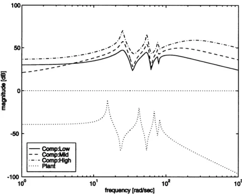
4-1 MIMO plant system of the 4-mode flexible MACE model ... . 121 4-2 Singular value plots of the transfer matrix from the control inputs to

the sensor outputs of the MIMO plant with the frequency uncertainty changes . . . .. . 123 4-3 Singular value plots of the transfer matrix from the control inputs to

the sensor outputs of the MIMO plant with the primary gimbal angle changes . . . .. . 123 4-4 Singular value plots of the LQG compensators and the plant system . 127 4-5 Performance of the LQG compensators . ... 128 4-6 Comparison of the LQG costs of the LQG compensators ... . 131 4-7 LQG cost of the closed loop system with the low authority LQG

com-pensator . . . .. . 132 4-8 LQG cost of the closed loop system with the middle authority LQG

com pensator . . . .. . . . 133 4-9 LQG cost of the closed loop system with the high authority LQG

com-pensator . . . .. . 134 4-10 Nichols plot : High authority LQG compensator and the plant system

perturbed by frequency uncertainty . ... 135 4-11 Nichols plot : High authority LQG compensator and the plant system

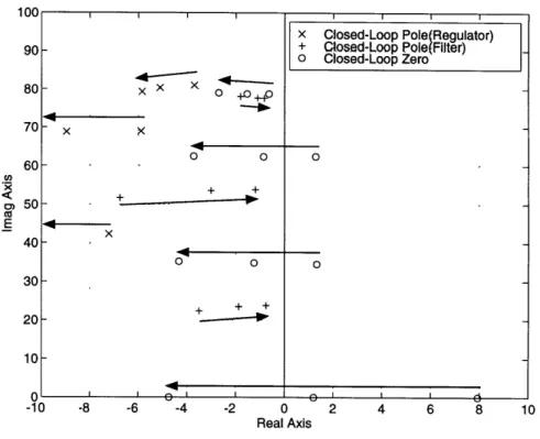
4-12 Sensitivity plot ( a[l + G,, K] ) : High authority LQG compensator . 137 4-13 Changes of the nominal LQG cost as a function of the control authority139 4-14 Singular value plots of the low authority MM compensators and the

plant system . . . 141 4-15 Performance of the low authority MM compensators ... 142 4-16 Comparison of the LQG costs of the low authority MM compensators 144 4-17 LQG cost of the closed loop system with the low authority FU-MM

compensator ... ... .. 145

4-18 LQG cost of the closed loop system with the low authority

FU&PG-M FU&PG-M compensator ... 146

4-19 Singular value plots of the high authority MM compensators and the plant system . . . 148 4-20 Performance of the high authority MM compensators ... 149 4-21 Comparison of the LQG costs of the high authority MM compensators 151 4-22 LQG cost of the closed loop system with the high authority FU-MM

com pensator . . . 152 4-23 LQG cost of the closed loop system with the high authority

FU&PG-MM compensator ... ... 153

4-24 Nichols plot : High authority FU&PG-MM compensator and the plant system perturbed by frequency uncertainty . ... 154 4-25 Nichols plot : High authority FU&PG-MM compensator and the plant

system perturbed by primary gimbal average angle . ... 155 4-26 Sensitivity plot ( a[I + G,, K] ) : High authority FU&PG-MM

List of Tables

2.1 Physical values of the 4-mode free-free flexible beam ... 42 2.2 Z-bending modes of the 4-mode free-free flexible beam . ... 46 2.3 Z-bending modes of the nominal 0-g model of the MACE test article. 46 2.4 Configuration of the SISO plant system of the 4-mode free-free flexible

beam . . . .. .. . 47 2.5 Summary of the LQG designs for the SISO plant system of the 4-mode

free-free flexible beam ... 53 2.6 Summary of the MM designs for the SISO plant system of the 4-mode

free-free flexible beam ... 65

3.1 Additional physical values of the 4-mode flexible MACE model . . .. 80

3.2 Nominal bending modes of the 4-mode flexible MACE model .... . 81 3.3 Configuration of the SISO plant system of the 4-mode flexible MACE

m odel . . . . . . .. .. . 82 3.4 Plant pole-zero frequencies with the primary gimbal angle changes . . 84 3.5 Summary of the LQG designs for the SISO plant system of the 4-mode

flexible MACE model ... 87

3.6 Summary of the MM designs for the SISO plant system of the 4-mode

flexible M ACE ... 99

4.1 Configuration of the MIMO plant system of the 4-mode flexible MACE

model . ... ... 122

4.2 Nominal bending modes of the 4-mode flexible MACE model ... 122

4.3 Summary of the LQG designs for the MIMO, 4-mode flexible MACE m odel .. ... .... . .. .. . ... . ... . . . .. 126 4.4 Stability boundaries of the LQG compensators . ... 129 4.5 Summary of the MM designs for the MIMO, 4-mode flexible MACE

m odel ... ... ... 139

4.6 Stability boundaries of the low authority MM compensators .... . 140 4.7 Stability boundaries of the high authority MM compensators ... 147

Chapter 1

Introduction

Future space systems will require high robustness of the control system as well as high performance because of their two major features: lightly damped structural dy-namics and nonlinear inertia properties induced by the large motion of articulating sensor heads and antennas. Effective robust control design techniques are needed to satisfy the performance requirements of future space systems in the presence of model uncertainties and nonlinear changes in their inertia properties.

In this introduction, the development of robust control design techniques is re-viewed at first. The review covers the comparative study of robust control design techniques made by the research team in the Space Engineering Research Center (SERC) at the Massachusetts Institute of Technology (MIT). Secondly, the Mid-deck Active Control Experiment (MACE) program, conducted by the research team at SERC, is introduced as the most aggressive research to develop a control design methodology for future space systems. Finally, the motivation and objectives of this study are presented in the last section.

1.1

Robust Control Design techniques

In control designs, trade-offs between properties of a compensator are usually un-avoidable. A trade-off between controller's nominal performance and sensitivity to

uncertainty is a typical example of the trade-offs in control designs. Simple and ef-fective means to evaluate controllers are needed to perform these trade-offs.

The Linear Quadratic Regulator (LQR) technique was developed to allow con-trol designers to conduct designs in a practical way [1]. Through specifying weights on each of the state and control variables, the LQR technique provides the optimal state feedback gains which minimize an LQR cost functional, i.e. a weighted sum of quadratic state and control variables. An LQR controller is found by solving an alge-braic Riccati equation and it guarantees stability margins, ±60deg phase margin and

-6dB gain margin, in each channel [2]. However, an LQR controller is not practical,

because all state variables cannot be measured in most design cases.

To allow sensor output feedback, Linear Quadratic Gaussian (LQG) control was introduced in the 1960s by combining an LQ regulator and a Kalman filter (KF), and had matured as a practical control design technique by the beginning of the 1970s [3]. Although an LQG solution is easily obtained by solving two decoupled al-gebraic Riccati equations, the LQG technique does not guarantee robust stability [4]. A laborious iterative design procedure like tuning the weights on the performance outputs and sensor noises has to be performed before obtaining an adequate compen-sator to satisfy stability requirements for off-nominal factors. This drawback of the LQG technique led control researchers and designers to demand robust control design techniques in the modern linear control theory.

In the following two decades, many robust control design techniques were devel-oped mainly by modifying the LQG technique. The robust control techniques, such as LQG/Loop Transfer Recovery (LQR/LTR) [5, 6], Trajectory Sensitivity Optimiza-tion (TSO) [7], Sensitivity Weighted LQG (SWLQG) [8], Parameter Robust LQG [9], Maximum Entropy [10], and Multiple Model (MM) [11], are based on the LQG tech-nique.

On the other hand, new approaches were also conducted to obtain a robust con-troller. The - technique has been studied most vigorously in the last fifteen years [12, 13]. The 7-e technique is based on the ?, norm of the closed loop transfer function matrix from disturbance to performance, while the LQG technique is based

on the quadratic (W2) norm. Although the 7F, technique starts with a concept dif-ferent from that of the LQG technique, it was proved that the 7, technique includes the LQG technique as a special case [13].

The most remarkable feature of the 4%, formulation is that the compensator pro-vides outstanding guaranteed robustness. However, this robustness is achieved with a large loss of nominal performance, and an 4, compensator is too conservative in many control design cases because its resulting robustness bounds far exceed the targeted bounds. Thus, the current issue in the i,, technique is the reduction of the conservatism of robustness [14].

The answer for the question of which robust control technique should be adopted totally depends on the plant system and the type of off-nominal factors. Grocott performed a comparative study of nine robust control techniques for flexible space structure systems, and demonstrated the effectiveness of SWLQG, ME, MM, and Popov Control Synthesis [15] and the extreme conservatism of W4, synthesis and p-synthesis [16]. In particular, he emphasized the superiority of the MM technique for a plant system with real parametric uncertainties.

1.2

Middeck Active Control Experiment (MACE)

The recent development of robust control design techniques allows engineers to design high performance controllers. However, control designers can appreciate the benefit of robust control techniques, only if they have precise dynamic models of a plant system including the associated off-nominal models. In some control design cases, measurement data of an actual plant is available. Unfortunately, it is impossible for space system designers to have a precise dynamic model of a space system in a weightless state before the system is launched, because there is no way to perfectly simulate zero-gravity (0-g) conditions on the ground. This is a significant problem in designing a control system particularly for flexible space structure systems, because these systems have complex dynamic modes due to a large number of degrees of

free-Suspension Cable

Strain Gages Strut

Secondary Gimal Secondary Payload

+Y

Reaction Wheel Assembly

Primary Gimbal Primary Payload Rate Gyro Platform

1.7 m

Figure 1-1: Middeck Active Control Experiment (MACE) test article (ground exper-iment configuration in 1-g)

dom in their dynamics.

The Middeck Active Control Experiment (MACE) program was conducted by the research team in the Space Engineering Research Center (SERC) at the Massachusetts Institute of Technology (MIT) in order to establish a control design methodology for space systems which have interaction between their attitude and pointing control and their structural dynamics [17]. The main technical challenges in the MACE program are to develop a precise analytical O-g model with a combination of Finite Element Method [18] and 1-g measurement data of a plant system, and to design high per-formance compensators for O-g implementation using several robust control design techniques.

The MACE test article, shown in Figure 1-1, was developed as a typical flexible space structure system. It consists of four flexible struts, a three-axis reaction wheel assembly, and two payloads: the primary payload and secondary payload. The reac-tion wheel assembly is equipped at the center of the structure and controls the bus attitude in the three axis. Each payload is controlled by a two-axis (X and Z axis)

gimbal at each end of the connected struts. The actuator system, consisting of the reaction wheel assembly and two gimbals, allows the MACE test article to control each section separately and prevents it from being destabilized by the interaction between its control and structural dynamics. The sensor system includes three rate gyros collocated with the reaction wheel assembly, two (X and Z axis) rate gyros in the primary payload, and two (X and Z axis) encoders in each gimbal. In total, the MACE test article has seven actuator inputs and nine sensor outputs (three inertial angels of the bus body, two inertial angles of the primary payload, and two relative angles at each gimbal system). The secondary payload can simulate an uncollocated disturbance source. Large motion of the payloads causes nonlinear changes of the MACE test article's inertia properties.

The MACE program was in its climax when the 0-g dynamic model measurements and control experiments were operated on the United States Space Shuttle Endeavor during the STS-67 mission in May 1995. The flight experiments validated the control design methodology developed by the research team of SERC. Detailed results will be reported by the research team in the near future.

1.3

Motivation, Objectives, and Outline

The control objective in the MACE program was to maintain the inertial pointing of the primary payload while the second payload was undergoing either broad or nar-rowband excitation. The frequency uncertainty, based on the comparison between a 1-g analytical model and a 1-g measurement model, was used as the off-nominal factor in the MACE control design.

Most space systems have large antennas and sensor heads which are required to have tracking modes as well as pointing modes. Large-angle tracking causes the iner-tia properties to change in a nonlinear way. These nonlinear ineriner-tia property changes can destabilize the closed loop control system when it is designed without their con-sideration. Therefore, future space systems require a reliable and high performance

control system, which can deal with nonlinear inertia properties as well as model uncertainties.

There are two major design approaches to satisfy this requirement: nonlinear control and linear, robust control. Nonlinear control has been vigorously studied by many researchers lately, because all the plant systems in practical control designs have nonlinear properties. Feedback Linearization is a typical nonlinear control tech-nique [19]. Feedback Linearization techtech-nique provides excellent performance for a nonlinear plant system, when a precise nonlinear mathematical model of the nonlin-ear plant system is obtained. However, this technique cannot be applied to all types of nonlinear systems, and it is difficult to develop a precise nonlinear mathemati-cal model in practimathemati-cal designs. Due to poor robustness of a Feedback Linearization controller, an inaccurate nonlinear model causes large performance degradation or destabilization [20]. Furthermore, full states have to be measured in a Feedback Lin-earization controller. In many plants including the MACE test article, it is impossible to measure full states. Therefore, many researchers are currently making great ef-forts to develop nonlinear observers. However, they are still immature because they all have drawbacks, such as necessity of an exact nonlinear mathematical model and heavy computational loads [21].

Adaptive Control is another typical nonlinear control technique. The basic concept of Adaptive Control is to estimate plant uncertainties based on on-line measurement data and to adjust gains in the controller. Since there is unknown variation of a plant in many practical designs, Adaptive Control has been expected to be useful in practical application. However, an instability problem of existing Adaptive Control algorithms was pointed out by Rohrs et al [22]. Although research on the Robust Adaptive Control Problem has been vigorously pursued since then, no effective mod-ification has been proposed yet [23].

Although linear control techniques are usually applied at each operating point, Gain Scheduled Control is categorized as one of the nonlinear control techniques. In spite of a lack of strong theoretical background, this technique is applied to many practical problems. The main drawback of this technique is no guarantee of the

stabil-ity and performance of the system at intermediate points [24]. To maintain stabilstabil-ity robustness, the system needs to vary sufficiently slowly [23]. Since space systems including the MACE test article are not usually required to make quick motion, Gain Scheduled Control is applicable to them. However, an onboard processor needs to have a sufficiently large capacity because several sets of gains need to be installed in it.

As mentioned above, nonlinear control techniques are still immature and require high computational performance and large capacity of an onboard processor. On the other hand, linear, robust control techniques are reliable because they are based on mature linear control theories. Some robust control techniques, such as Multiple Model, 4,,, synthesis, -synthesis, and Popov Control synthesis, guarantee robust stability for designated off-nominal conditions. Furthermore, requirements for a pro-cessor are not excessive. Therefore, it is a reasonable approach to apply linear, robust control techniques to a nonlinear plant at first and to examine the performance limit of linear, robust controllers. The main issue in implementing a robust control design is a trade-off between controller's nominal performance and robustness. The question of which robust control design is the most effective depends on properties of a plant system. Therefore, it is very important to find the most effective robust technique to a plant system that provides a large robustness gain at a sacrifice of a small nominal performance loss.

The objective of this research is to examine the effectiveness of a linear, robust control technique at designing high performance compensators which stabilize a space structure system with nonlinear inertia properties. The Multiple Model (MM) tech-nique is examined as one of the most effective robust control design techtech-niques for a space structure system, while the MACE test article is adopted as a typical space structure system.

This thesis consists of three main chapters. In Chapter 2, the LQG and MM tech-niques are introduced and applied to a sample structural system, the 4-mode free-free flexible beam, to understand the destabilization mechanisms associated with a lightly damped structural plant. The development of the analytical model of the 4-mode

free-free flexible beam using the Finite Element Method [18] is also presented in this chapter. Chapter 3 presents SISO designs for the MACE test article with four Z-axis bending modes to examine the influence of nonlinear inertia properties caused by different primary payload average angles and the effectiveness of the MM technique. Two off-nominal factors are considered: ±10% frequency uncertainty in the second Z-axis bending mode and ±45deg primary gimbal average angles. The frequency un-certainty is caused by model errors and is limited in the second Z-axis bending mode in this SISO design case to mainly examine the effect of the other off-nominal factor,

i.e. the primary gimbal average angle. Large changes of the primary gimbal angle

result in nonlinear changes of the MACE test article's inertia properties.

Finally, in Chapter 4, MIMO designs for the MACE test article are performed as a more realistic design case. The secondary payload acts as an uncollocated distur-bance source. Two off-nominal factors are also considered in MIMO designs: ±2.5% frequency uncertainty in all Z-axis bending modes and ±45deg primary gimbal aver-age angles.

Chapter

2

Control Design Techniques and

Sample Designs

A compensator for future space systems must be robust to their two major off-nominal factors, i.e. uncertainty in structural dynamics and geometric nonlinearity. The Lin-ear Quadratic Gaussian (LQG) is powerful in control designs for future space systems because of its practicality; a high authority compensator is easily obtained by solving two decoupled algebraic Riccati equations. However, this technique cannot guarantee robust stability. Therefore, robust control techniques need to be applied to future space systems. The Multiple Model (MM) technique can be used in control designs for future space systems as the most effective robust control technique.

The objectives of this chapter are to introduce the LQG and MM technique and to examine basic properties of an LQG and MM compensator for space structural systems through sample designs for a free-free beam.

2.1

Linear Quadratic Gaussian (LQG)

To allow sensor output feedback, Linear Quadratic Gaussian (LQG) control was in-troduced as a practical control design technique by combining an LQ regulator and a Kalman filter (KF). Although an LQG solution is easily obtained by solving two

decoupled algebraic Riccati equations, the LQG technique does not guarantee robust stability. This drawback of the LQG technique led control researchers and designers to demand robust control design techniques. Many robust control techniques includ-ing Multiple Model (MM) were developed based on the LQG technique. Therefore, the LQG technique is applied to many engineering problems as a basic linear control technique. In this study, LQG compensators are used as an initial compensator in a MM design and compared with resulting MM compensators. This section presents the formulation of the LQG technique and the design strategy in applying the LQG technique to the design problems presented in this study.

2.1.1

Formulation

Control design always starts at modeling the plant. The Linear Quadratic Gaussian (LQG) method is no exception [3]. A linear time invariant equation has to be formu-lated. The following general form is often adapted in order to generalize W-2 and W,.

design techniques [12, 13].

x = Ax + Bw + Bou (2.1)

z = Cz + Dzw + Dzu

y = CYx + Dyw + DYuu

where x, z, and y are a state variable vector, a performance vector, and an output vector, respectively. w and u are a disturbance vector and a control variable vector, respectively.

The open loop transfer functions from the inputs, w and u, to the outputs, z and

y, are given by

Gzw(s) = Cz(sI- A)-1B, + Dz, (2.2)

Figure 2-1: General control system

= C(sI = C,(I

-A)- 1B, + D,,, A)-'B, + Dy,.

Figure 2-1 shows the closed loop system with the compensator, K(s). The closed loop performance transfer function from w to z is given by

Gcl(s) = Gz,(s) - Gzu(s)K(s) [I + GY,(s)K(s) ]- Gy,(s). (2.3)

The compensator, K(s), is represented as

~ = Axc + Bcy, (2.4)

U = -Ccxc,

where xc is a state variable vector estimated by the filter.

Then, by using the representation of the closed loop system, the plant system, which is equivalent to Equation (2.1), is written in the augmented state space repre-sentation, x = A + Bw

z =

+ bw

~1~-where

A=

A

-BCc

BC, A - BcD,,C

C =

C-DZUC

D

D,

By using the representation above, the closed loop transfer function, which is equiv-alent to Equation (2.3), is given by

Gil(s) = C(sI - A)-B + D. _(2.6)

The smaller the gain of the closed loop transfer function, the better the closed loop system rejects disturbances. Therefore, the objective of control design is to find a compensator which minimizes the closed loop transfer function, G (jw).

There are many ways to evaluate the magnitude of Gcl(jw). The 7t2 norm is adopted in the LQG technique, while the 7&, norm is used in the h,, technique [25].

The 7t2 norm is defined as

1 +oo

|Gc(s) 12 = -trace] Gcl(jw)G*z(jw) dw

2 t27r G0

= trace

_/OOOl"l

(2.7)

In the equation above, the Parseval theory is applied to transfer the integration with respect to frequency to the integration with respect to time [26].

There is no general analytic solution of the integration above, because the solution depends on the input to the closed loop system. In the LQG technique, an impulse

input is adopted to have a specific solution. Since the time domain transfer function of the closed loop system, which is given by Equation (2.6), for an impulse input is

Gc(t) = C exp(At)B, (2.8)

then the 72 norm of the transfer function is given by [27]

IIGI(s)

j

= _{trace [CT],} (2.9)

where

Q

A

In the LQG technique, the 72 norm defined above is adopted as the LQG cost func-tional, J, which includes both state and control components.

On the other hand, applying stochastic inputs to the closed loop system also gives the same cost functional for the LQG problem.

J = |Ge112 =lim {T zz dt T-oo T 0 lioom E fT [Xr R xx x + 2x R x u u + UT R uuu , dt

,

where Dz,, = 0 to guarantee finite 72 norm. E is the expectation operator. The weights for the state variables and the control variables are defined as

(2.13)

F Rx

L

RXU

D

Note that R and , need to be a semi-positive definite matrix (R > 0) and a positive

definite matrix (R, > 0), respectively.

Now the optimum gains, F and H, which minimize the cost functional in the LQG problem, Equation (2.9) or Equation (2.12), are given by

F = R- R + BTP] (2.14)

H = [QCT + Vy] VI1, (2.15)

where P and Q are the solutions of the following two decoupled algebraic Riccati equations,

O = PA + ATP + Rxx - [PBu + Rxu] R- [R + B TP] (2.16)

o

and the weights for the estimated state variables and the sensor noises are defined as

V Vy BBT T D . (2.18)

VT VY DYW

V and Vyy need to be a semi-positive definite matrix (V > 0) and a positive definite

matrix (V > 0), respectively.

The LQG compensator is composed by applying the LQG optimum gain set, Equation (2.14) and Equation (2.15), to the compensator, K(s) represented by Equa-tion (2.4). Thus, the system matrices of the LQG compensator are given by

Ac = A- B,F- HCy + BuDyuC (2.19)

BC =H

cc = F.

The most remarkable feature of the LQG compensator is the separation princi-ple [28]. The LQG compensator can be separated into the LQR (Linear Quadratic Regulator) and the KF (Kalman Filter). However, the LQG compensator does not have robustness guarantees [4], while the LQR and KF individually have +60deg

phase margin in each channel, independently and simultaneously, and [2, +o] gain margin [2].

By using the estimation error vector, e = x - xc, and the system matrices of the

LQG compensator given by Equation (2.19), the augmented state representation of the closed loop system, Equation (2.5), can be reformulated as

d x A - BF B F x B,

=

+

(2.20)

dt e 0 A - HCY L eJ B, - HD,,y

= Cz - DzuF DzuF

]

Note that D = D = 0 for the LQG problem. Therefore, the closed loop poles are given by

det [AI- (A - BuF)] = : LQR poles (2.21)

det [AI- (A- HC)] = 0: KF poles. (2.22)

Using the equations above, the LQR poles and KF poles can be specified respec-tively.

2.1.2

Design Strategy

The most outstanding feature of the LQG design technique is the systematic design procedure made possible through the tuning of the state, control, and filter weights. Tuning the weights determines the properties of the compensator. In the general form of the plant system, Cz, Dzu, and Dy matrices correspond to the state weights, the control weights, and the filter weights, respectively. The weights are determined from these matrices by Equation (2.13) and Equation (2.18).

In most of control design cases, however, the number of the weights easily becomes large. In particular, the number of state variables in the flexible space structure prob-lem, which is the main topic of this study, is quite large. This leads control designers

to laborious trial-and-error design procedures before getting adequate compensators which satisfy the design requirements. Therefore, effective ways of tuning the weights are required.

In this study, the following procedure is adopted for tuning the weights in the LQG problem.

1. Since only relative ratios among the weights are meaningful, the B,, Cz, Dz,

and D, matrices are set in the first step such that

B = Bo(nx n,) O(nxxn)

]

Dy, =

[

]

where p and 0 are scalar weights on the control variables and the sensor noises, respectively. oi, pj, and Ok _{are individual scalar weights on each component of}

the state and control variables, and the sensor noises, respectively. All the in-dividual scalar weights are set to one, at first. The diag(.) indicates a square matrix which has the specified individual scalar weights as diagonal entries.

nx, n~, and ny are the order of the state variable vector, x, the control variable vector, u, and the output variable vector, y, respectively. nzx is the number of the state variables which are chosen as the components of the performance vector. n, and n, are the number of the process and sensor noises, respectively. Since the Cz and Dzu _{matrices mentioned above have a zero submatrix, they}

give a set of independent weights on the state variables and control variables, and zero weights on the cross product of the state and control variables. The weights on the state-control product play an important role in the robust control design. An adequate set of the weights on the state, control, and state-control

product provides good robustness. The sensitivity weighted LQG (SWLQG) is a robust control technique which positively uses the state-control product [8]. In this study, however, the state-control product is set to zero for simplicity.

The B, and Dy, also have a zero submatrix to make the process and sensor

noises uncorrelated; BD T, = 0.

2. Set a control scalar weight, p, and then find a disturbance scalar weight, 0, so that the following condition is satisfied.

* Balanced Weight Condition:

J1

J2

(2.27)

J4 J3'

where J1 = trace [PVxx]

J2 = trace [RxxQ]

J= trace [P(QC + VY)V-(V T + CYQ)]

J4= trace [(PBu + Rxu)R- (R T + BTp)Q

Note that J1 and J3 contribute to the LQG cost, Equation (2.9) or

Equa-tion (2.12), by the regulator part of the LQG compensator, and that J2 and J4

contribute to the LQG cost by the filter part of the LQG compensator. The LQG cost functional can be written by using J1, J2, J3, and J4.

J = J1 + J4 = J2 +J3

Therefore, satisfying the Balanced Weight Condition gives an LQG com-pensator which has an evenly-balanced regulator and filter cost contribution. Smaller control scalar weights give higher authority compensators. Control au-thority of the compensator corresponds to the bandwidth of the compensator; high authority compensators have high crossover frequency.

3. Change individual scalar weights, ai, pj, and 0_{k, in C, D,,, and D, in order to}

modulate cost contribution by the individual variables or sensor noises. Then, apply the Balanced Weight Condition to find a new disturbance scalar weight, 0. A heavier individual scalar weight on a particular variable or sensor noise makes its LQG cost contribution smaller. The analysis tools, such as the frequency response plot mentioned in Section 2.3.2, are helpful to obtain information on individual variables and sensor noises. Repeat this step until a desirable LQG compensator is obtained.

The tuning of the weights is the most laborious process in a LQG design. The procedure described above is one of the measures to reduce the laboriousness.

2.2

Multiple Model (MM) Method

The Multiple Model (MM) method can be based on the LQR or the LQG [11, 29] problems. In this study, the MM method based on the LQG is adopted, because it is more practical than that based on the LQR.

The most remarkable feature of the MM method is that it provides guaranteed robustness for designers, through direct specification of off-nominal design points, with relatively small loss in nominal performance [16]. Compensators designed with the MM method guarantee stability at a nominal design point and every specified off-nominal design point but do not guarantee stability outside of the design points. The principle of the MM method is to find a compensator which stabilizes every design point plant system and minimizes a weighted sum of the LQG costs of each design point. While the principle of the MM method is easy, there is no analytical equation like the algebraic Riccati equations in LQG, Equations (2.16) and (2.17), which can be solved analytically. Therefore, numerical nonlinear multivariable opti-mization methods, such as the Newton method or the Quasi-Newton method [30, 31], need to be introduced to find the solution. This results in a large amount of calcula-tion load and does not guarantee convergence to an optimal solucalcula-tion.

2.2.1

Formulation

Because the Multiple Model (MM) design technique is based on the LQG design technique, the formulation of the MM method starts at the formulation of the LQG method developed in Section 2.1.1.

Since the LQG is a design technique based on a linear, time-invariant plant system, there are two kinds of off-nominal sources: uncertainty and unmodeled dynamics. Nonlinearity is one of the unmodeled dynamics which is removed in the process of linearization. The MM method provides linear time invariant compensators which stabilize off-nominal plant systems by increasing robustness of the compensators.

At first, some off-nominal design points based on off-nominal factors of the plant system have to be selected. The linear time invariant state equations can be set at

each design point including the nominal design point as follows: x = Aix + B,, w + Bu z = Cz, x (2.28) + Dzuiu y = Cx + D w + Dy,u,

where the subscript "i" refers to the design points. Note that Dz,, = 0 for the LQG problem.

With the compensator, K(s),

:c = Axc + Bcy _(2.29)

U = -Ccxc

the augmented state equations at each design point can be written as

X = Ai. + Biw _(2.30) z= Ci, where Ai - Bu, c BcCy, Ac - BDyu, Cc B, BcDywi Cz, -Dzu,Cc

1

Ai=

The LQG cost can be determined by the system matrices of the augmented state equations. Thus, the weighted sum of the LQG costs at the design points is given by

DP

Jo = E trace (~'4Q f] , (2.31)

i=1

where

/i

'nDP

/

Qi

AQ + QjAT + BiBT = 0. (2.32)

Now, the MM problem is to find the matrix set, Ac, Bc, and Cc, which minimizes the weighted sum of the LQG costs, Ja, under the condition of the Lyapunov equa-tions, Equation (2.32).

By using the Lagrange multipliers, Pi, the weighted sum of the LQG costs can be written as

nDP

Ja =

Za

i=1

The partial derivatives of Ja with respect to the variable matrices, Ac, B,, and C', are derived as follows:

tJa "DP OA = 3[(P)T + (PQ)22]i (2.34) J "DP S i=1 SJa nD TP EA [D DzuC 2 + Q22) - D[ (Q1 + 2 Q12) -B{(QP)T + (PQ)12)} - D T BT(Qp) + (PQ)22 ]i,(2.36) ZDzz(2

where (')11, (')12, ()21, and (')22 are n, x n. matrix entries of the indicated matrix. For instance,

PQ (PQ)11 (PQ)12

(PQ)₂₁ (PQ)22

Refer to Appendix A for the derivations of the derivatives.

For the optimum solution of the matrix set, the following partial derivative has to be zero. That is,

aJ

- =- Pi + AiTP + CZT C = 0. (2.37)

OQ

This is another Lyapunov equation with respect to the Lagrange multipliers, Pi. The solution, P, is used to evaluate the partial derivatives, Equation (2.34), Equa-tion (2.35), and EquaEqua-tion (2.36).

2.2.2

Design Strategy

Since there is no analytical solution of the MM problem, numerical optimization methods, such as the Newton method and the quasi-Newton method, need to be used to get the optimum solution, which minimizes the weighted sum of the LQG costs. In either method, an adequate initial matrix set, Ao, Bo, and CO,, has to be chosen to start the iterative calculation. The LQG solution can be used as the initial matrix set as long as it is stable for each design point. In this study, the following procedure is adopted to obtain the MM solution.

1. An LQG solution is chosen as an initial matrix set. Therefore, the design parameters, such as the state, control, and filter weights, are the same as those used to find the LQG compensator. The LQG solution is obtained by following the procedure described in Section 2.1.2.

2. Set the cost weights, /i. A heavier cost weight gives a wider stable region around the corresponding design point.

3. All closed loop systems in the MM design procedure, which consist of the plant system at each design point and the compensator in the middle of the iterative calculation, must be stable. Therefore, at the start of the calculation, tem-porary off-nominal design points, which are inside of the stable region around the nominal design point provided by the initial compensator, need to be set. The optimum solution of this temporary design step expands the stable region around the nominal design point, and then can be used as the initial matrix set for the next design step. In the next design step, the temporary off-nominal de-sign points are moved toward the final off-nominal dede-sign points. The solution for the final off-nominal design point is the targeted MM solution.

The design procedure described above is called the progressive method. This method can be one of the measures to avoid obtaining local minima in the numerical opti-mization process instead of the global minimum. In this study, the effectiveness of this method is also examined.

2.3

Sample Designs

The sample control design is posed in order to investigate basic properties of the plant system and the compensators designed with the LQG technique and the MM technique. The most important thing in the sample design is to understand the mech-anism of destabilization of the closed loop system due to the frequency uncertainty of the plant system.

The plant system in the sample design should be as simple as possible without losing its basic properties. A single input and single output (SISO) plant system of a free-free flexible beam is selected as the sample plant system.

2.3.1

_{Plant System for the Sample Designs}

The Middeck Active Control Experiment (MACE) test article was developed as a typical model of a future flexible space structure system, such as space stations and space platforms. The main feature of this type of system is lightly damped structural dynamics. Poles and zeros of the plant system are alternately and successively located near the imaginary axis on the left half of the complex plane. This pole-zero location is deeply related to stability of the closed loop system.

In order to study this basic plant dynamic feature and compensators designed with LQG and MM, a free-free beam is selected in the sample designs. The free-free beam has similar physical properties to those of the MACE test article, such as mass distribution and stiffness of the struts. This beam, however, does not have gimbals like attached to the MACE test article.

The model for the sample design needs to have a few modes at least to examine the lightly damped pole-zero structure. The plant system selected in the sample designs is modeled in the X-Y plane, and has four Z-bending modes. The Finite Element Method (FEM) is used to develop the analytical model of the free-free beam [18].

The sample model consists of four flexible struts, one heavier center node mass, two intermediate node masses, and two end node masses. The masses are modeled

Z X

q2 q5 q8 qll q14

q3 q l q6 q4 q9 .q7 q12 q 1 5 __q 13

Strut#1 Strut#2 Strut#3 Strut#4

End Node#1 Node#1 Center Node Node#2 End Node#2

Figure 2-2: Sample model; 4-mode free-free flexible beam

as rigid. Figure 2-2 shows the sample model, and Table 2.1 shows physical values of the sample model. The flexible struts have similar physical properties to those of the MACE test article.

As shown in Figure 2-2, each strut has a reference point at each end, and each reference point has three degrees of freedom resulting in six degrees of freedom for each

strut (xl, yl, 1, x2, Y2, and 02). Each rigid mass has three degrees of freedom (r,, yr, and Or), which correspond to the degrees of freedom of the struts by connecting it

to the ends of the struts. The 4-mode free-free flexible beam is assembled from these elements as illustrated in Figure 2-2 and has 15 degrees of freedom. Eventually, four Z-bending modes are extracted by truncating the 11 other modes.

The equations of motion in the physical reference coordinates are given by

M + 0 + [R P, (2.38)

where q is the displacement variable vector, [Ai] is the geometry matrix of i-th element, and

[M] = [i]T [i] [i]

I^IIIIIIYLIII~-Table 2.1: Physical values of the 4-mode free-free flexible beam

]

[

= [Ai]T fi.

The mass [Tmi] and stiffness [ki] matrices for the flexible struts in the X-Y plane are given by 140 0 0 70 0 0 0 156 22L 0 54 -13L mL 0 22L 4L2 0 13L -3L 2

[mi]

(2.40)

item symbol values

Center Node : Mass Mc 14.35 kg

Moment of Inertia (Z-axis) Izc 2.038 x 10-1 kg m2

Intermediate Nodes : Mass MNj (j = 1, 2) 1.300 kg Moment of Inertia (Z-axis) IzNj (j = 1, 2) 9.521 x 10-3 _{kg m}2

End Nodes : Mass MEj (j = 1, 2) 7.062 kg

Moment of Inertia (Z-axis) IzEj (j = 1, 2) 1.014 x 10-1 kg m2

Struts : Density pj (j = 1, 2, 3, 4) 3099 kg/m3

Length Lj 0.2643 m

Modulus of Elasticity Ej 2.578 x 109 N/m 2

Cross-sectional Area Moment of Inertia Izj 2.140 x 10-8 m4

Cross-sectional Area Aj 2.560 x 10-4 _m2

-3L 2

2

0

0

0

0

[ks]

L

(L)2

0

0

(;L2

0

0

where r is the radius of gyration of the cross-sectional area and is given by r = . Im is the cross-sectional area moment of inertia, and A is the cross-sectional area.

The damping matrices, [ri], for the flexible elements are easily determined by using the modal coordinates introduced later.

The [~Yii], [Ei], and [ki] matrices for the rigid mass elements in the X-Y plane are given by mr 0 0 [Li] = 0 m 0 (2.42) 0 0 Iz [ri] = [0](3x3) (2.43) [ki]= [0](33) (2.44)

The physical reference coordinates are intuitive for understanding physical mo-tion of the beam. They, however, are not suitable for control design for the plant with parametric uncertainties in the natural frequencies of its bending modes, be-cause modal information is implicitly contained in the system matrices of the state equations. The modal coordinates are more convenient in designing compensators for the flexible structure system because the system matrices are expressed with modal parameters explicitly.

The transformation with the mode shape matrix, (D, defined below gives the fol-lowing equations of motion in modal coordinates.

I. + 2 [(] [Q] #j + [Q]2 = DT, (2.45)

where 77 is a modal variable vector and

[(] = diag((j) [Q] = diag(wNj).

The diag(.) indicates a square matrix which has a specified vector as diagonal entries.

(j and wNj denote the damping ratios and the natural frequencies of the j-th

Z-bending mode of the sample plant, respectively. Since the sample model has four modes, [(] and [Q] are 4 x 4 matrices in the sample designs in this section.

The mode shape matrix, 1, needs to satisfy the following relations:

q= 4,71;

qT [ 4) = I; (2.46)

DT[

4I

=

2 [(] [Q

4)T[_j = [Q]2

Now each mode can be explicitly specified.

The linear, time-invariant state equations based on the modal variables can be derived from the equations of motion, Equation (2.45).

d

[

dt _{_} 2 _-2(Q

( )T b

C

0

[l

where F = bu, and u is a control variable. Cd and C, correspond to the displacement

and rate sensors, respectively.

with uncertainties in natural frequencies is given by

0 _{I 0 0}

Q2 -2(Q A

L

(2.48)

where (6Q) = diag(6wNj).

Since a typical value of damping ratios, (j, of the space structure is in the order of 0.01, the uncertainty matrix, AA, behaves in a manner of a rank 1 matrix. This implies loss of exact information of the uncertainties.

On the other hand, the following representation enables the uncertainty matrix to keep rank 2. Therefore, the exact information of the uncertainties can be kept.

A=

-L Q /--(

Q I

(2.49)

where /I-2 = diag( 1 - ).

Then, the actual A matrix is given by

TZ- ]2 ]+"

-((Q)

-()QrI

-(2

(

2-(

)

new state variable vector, = Tij, gives the following new

d y = CA)

-s2~/r-¢

CdQ o

]

-(Q

_ ~L-- ~--l~---UIIIII~ -I II*Y-l--I--.--) - L-~II~L-LI-.~

S+

T-1

u

T Tb